Supervised Machine Learning Under Test-Time Resource Constraints: A Trade-off Between Accuracy and Cost

(1)

Washington University in St. Louis

Washington University Open Scholarship

All Theses and Dissertations (ETDs)

Summer 9-1-2014

Supervised Machine Learning Under Test-Time

Resource Constraints: A Trade-off Between

Accuracy and Cost

Zhixiang Xu

Washington University in St. Louis

Follow this and additional works at:https://openscholarship.wustl.edu/etd

This Dissertation is brought to you for free and open access by Washington University Open Scholarship. It has been accepted for inclusion in All Theses and Dissertations (ETDs) by an authorized administrator of Washington University Open Scholarship. For more information, please contact

[email protected].

Recommended Citation

Xu, Zhixiang, "Supervised Machine Learning Under Test-Time Resource Constraints: A Trade-off Between Accuracy and Cost" (2014).All Theses and Dissertations (ETDs). 1370.

(2)

Washington University in St. Louis School of Engineering and Applied Science Department of Computer Science and Engineering

Dissertation Examination Committee: Kilian Q. Weinberger, Chair

Sanmay Das Yasutaka Furukawa

Nan Lin Robert Pless Alice X. Zheng

Supervised Machine Learning Under Test-Time Resource Constraints: A Trade-off Between Accuracy and Cost

by

Zhixiang (Eddie) Xu

A dissertation presented to the Graduate School of Arts and Sciences of Washington University in partial fulfillment of the

requirements for the degree of Doctor of Philosophy

August 2014 Saint Louis, Missouri

(3)

c

(4)

List of Figures

1.1 Features and the feature vector of one hypothetical e-mail instance. . . 2 1.2 Decision boundaries of linear regression, linear SVM, kernel SVM and GBRT. 6 1.3 A schematic layout of Support Vector Machine (SVM). Blue and red dots are

training instances in a two dimensional feature space, and two colors indicate two classes. The solid black line is the decision boundary learned from the training data. Dotted dark lines are margins. Dots in light blue circles are support vectors. . . 7 1.4 A schematic layout of a classification decision tree. Blue and red shapes are

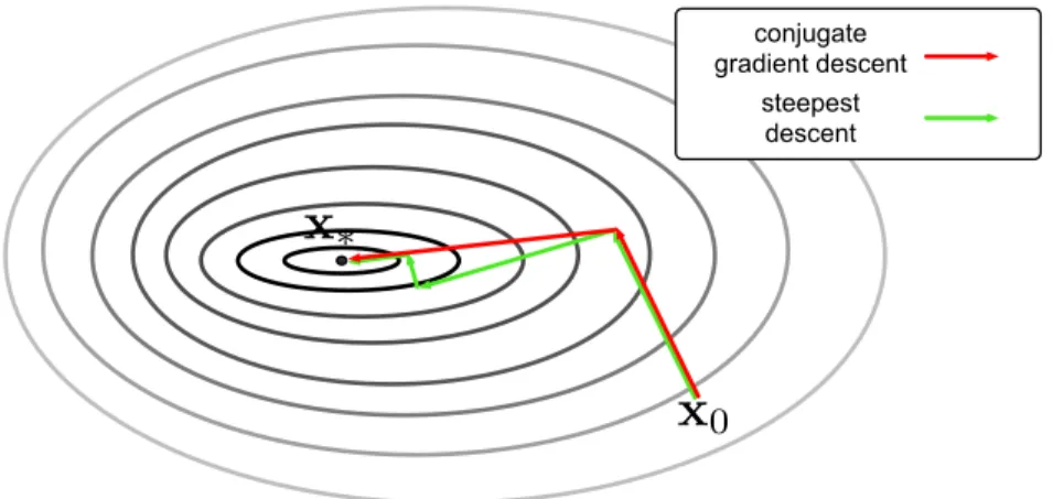
training instances in four classes (small red dot, large red dot, small blue dot and small blue rectangle). The black circles are decision tree internal nodes, and rectangles are leaf nodes. At each internal node, the decision tree partitions the input space by one of the features and a corresponding splitting value (e.g. radius < 2). Leaf nodes make predictions based on the instances in each leaf. . . 10 1.5 A schematic comparison of conjugate gradient descent (red) and steepest

de-scent with line search (green). . . 16 2.1 Gradient surface of a linear, a kernel and a GBRT classifier. (a) The linear

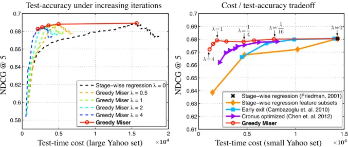
un-separable simulation data. Red dots and blue dots are from two different classes, and the task is binary classification. (b) The gradient surface of a linear classifier, which is a hyper-plane (c) The gradient surface of a kernel classifier. (d) The gradient surface of a GBRT classifier. . . 20 2.2 The NDCG@5 and the test-time cost of various classifier settings. Left: The

comparison of the original Stage-wise regression (λ = 0) and Greedy Miser under various feature-cost/accuracy trade-off settings (λ) on the full Yahoo set. The dashed lines represent the NDCG@5 as trees are added to the classi-fier. The red circles indicate the best scoring iteration on the validation data

set. Right: Comparisons with prior work on test-time optimized cascades on

the small Yahoo set. The cost-efficiency curve of Greedy Miser is consistently above prior work, reducing the cost, at similar ranking accuracy, by a factor of 10. . . 29

(7)

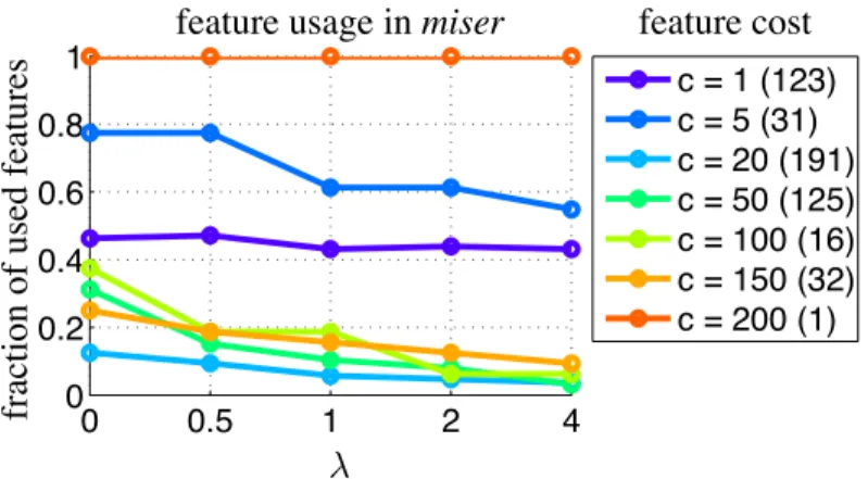
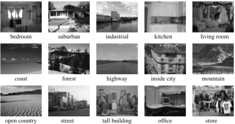
2.3 Features (grouped by costc) used in Greedy Miser with variousλ(the number of features in each cost group is indicated in parentheses in the legend). Most cheap features (c= 1) are extracted constantly in differentλ settings, whereas expensive features (c_≥5) are extracted more often whenλis small. The most expensive (and invaluable) feature c= 200 is always extracted. . . 31 2.4 Sample images of the Scene 15 classification task. . . 32 2.5 Accuracy as a function of CPU-cost during test-time. The curve is generated

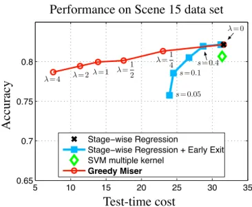
by gradually increasing λ. Greedy Miser champions the accuracy/cost trade-off and obtains similar accuracy as the SVM with multiple kernels with only half its test-time cost. . . 33 2.6 A schematic layout of Anytime Feature Representation Learning. Different

shaded areas indicate representations of different costs, the darker the costlier. During training time, SVM parametersw, bare saved every time a new feature

fi is extracted. During test-time, under budgets Be, Bf, we use the most

expensive triplet (φk,wk, bk) with costce(φk)≤Be and cf(φk)≤Bf. . . 40

2.7 A demonstration of our method on a synthetic data set (shown at left). As the feature representation is allowed to use more expensive features, AFR can better distinguish the test data of the two classes. At the bottom of each representation is the classification accuracies of the training/validation/testing data and the cost of the representation. The rightmost plot shows the values of SVM parametersw, b and hyper-parameter C at each iteration. . . 44 2.8 The accuracy/cost trade-off curves for a number of state-of-the-art algorithms

on the Yahoo! Learning to Rank Challenge data set. The cost is measured in units of the time required to evaluate one weak learner. . . 46 2.9 The accuracy/cost performance trade-off for different algorithms on the Scene

15 multi-class scene recognition problem. The cost is in units of CPU time. . 48 3.1 An illustration of two different techniques for learning under a test-time

re-source constraints. Circular nodes represent classifiers (with parameters β) and black squares predictions. The color of a classifier node indicates the number of inputs passing through it (darker means more). Left: CSCC, a classifier cascade that optimizes the average cost by rejecting easier inputs early. Right: CSTC, a tree that trains expert leaf classifiers specialized on subsets of the input space. . . 51 3.2 A schematic layout of a CSTC tree. Each node vk _{is associated with a weight}

vectorβk_{for prediction and a threshold}_θk_{to send instances to different parts}

of the tree. We solve forβk _and_θk_{that best balance the accuracy/cost}

trade-off for the whole tree. Each path in the CSTC tree is shown in a different color. . . 55 3.3 Schematic layout of our classifier cascade with four classifier nodes. All paths

(8)

3.4 CSTC on synthetic data. The box at left describes the data set. The rest of the figure shows the trained CSTC tree. At each node we show a plot of the predictions made by that classifier and the feature weight vector. The tree obtains a perfect (0%) test-error at the optimal cost of 12 units. . . 70 3.5 The test ranking accuracy (NDCG@5) and cost of various cost-sensitive

clas-sifiers. CSTC maintains its high retrieval accuracy significantly longer as the cost-budget is reduced. . . 71 3.6 The test ranking accuracy (Precision@5) and cost of various cascade classifiers

on the LTR-Skewed data set with high class imbalance. CSCC outperforms similar techniques, requiring less cost to achieve the same performance. . . . 72

3.7 Left: The pruned CSTC tree, trained on the Yahoo! LTR data set. The ratio

of features, grouped by cost, are shown for CSTC (center) and Cronus (right). The number of features in each cost group is indicated in parentheses in the legend. More expensive features (c _≥ 20) are gradually extracted deeper in the structure of each algorithm. . . 74 3.8 The ratio of features, grouped by cost, that are extracted at different depths of

CSCC (left), AND-OR (center) and Cronus (right). The number of features in each cost group is indicated in parentheses in the legend. . . 75 3.9 (Left) The pruned CSTC-tree generated from the Yahoo! Learning to Rank

data set. (Right) Jaccard similarity coefficient between classifiers within the learned CSTC tree. . . 76 4.1 Illustration of searching for a spaceV _{∈ R}2 _{that best approximates predictions}

P1 and P2 of training instances in R3 space. Neither V1 or V2, spanned by existing columns in the kernel matrix, is a good approximation. V∗ spanned by kernel columns computed from twoartificial support vectors is the optimal solution. . . 85 4.2 Illustration of each step of CVM on a synthetic data set. (a) Simulation inputs

from two classes (red and blue). By design, the two classes are not linear separable. (b) Decision boundary formed by a full SVM solution (black curve), and all support vectors (enlarged points). (c) A small subset of support vectors picked by LARS (cyan circles) and the compressed decision boundary formed by this subset of support vectors (gray curve). (d-h) Optimization iterations. The gradient support vectors are moved by the iterative optimization. The optimized decision boundary formed by gradient support vectors (green curve) gradually approaches the one formed by the full SVM solution. . . 87 4.3 Accuracy versus number of support vectors (in log scale). . . 89

(9)

List of Tables

(10)

Acknowledgments

First of all, I would like to express my sincerest gratitude to my advisor Kilian Weinberger. His patience during my early Ph.D. years, his trust in me during my dark days, and his support and guidance during my entire course of study have always encouraged me and shaped my scientific thinking of machine learning. Without him I could not have written this thesis.

I would like to thank my committee Sanmay Das, Yasutaka Furukawa, Nan Lin, Robert Pless and Alice Zheng for their comments and suggestions. Lots of work in this thesis benefited from their insightful thoughts and generous contributions. I would also like to especially thank Robert Pless for his guidance during the very first semester of my Ph.D. study and Alice Zheng for providing me a great internship opportunity at Microsoft Research.

I would like to thank Olivier Chapelle and Fei Sha for collaborating throughout and providing me experiences and ideas about the field of machine learning. I would also like to thank my co-authors Minmin Chen, Jake Gardener, Dor Kedem, Gao Huang, and Matt Kusner for exchanging ideas, discussing papers and picking up my mistakes. Especially many thanks to Minmin for sharing her knowledge and thoughts and Matt for helping all the time. I would also like to thank my lab mates, Wenlin Chen, Yuzong Liu, Stephen Tyree, Wenlin Wang and Quan Zhou for taking time to help me debugging, installing packages, and preparing talks and posters. Especially thanks to Stephen Tyree for reviewing this thesis and developing tools that lots of my work is based on.

I would like to thank my parents, Yudi Xu and Shumin Li for their love and support through-out my life. I am also very grateful for my grandparents Enqing Li and Xiuran Ma. Withthrough-out their careful parenting during my young age, I would not have gone so far.

Finally, I would like to thank my wife Wuxuan Xiang for sharing my ups and downs with love and support throughout the last few years.

Zhixiang (Eddie) Xu

Washington University in Saint Louis

(11)

ABSTRACT OF THE DISSERTATION

Supervised Machine Learning Under Test-Time Resource Constraints: A Trade-off Between Accuracy and Cost

by

Zhixiang (Eddie) Xu

Doctor of Philosophy in Computer Science Washington University in St. Louis, 2014

Research Advisor: Professor Kilian Q. Weinberger, Chair

The past decade has witnessed how the field of machine learning has established itself as a necessary component in several multi-billion-dollar industries. The real-world industrial setting introduces an interesting new problem to machine learning research: computational resources must be budgeted and cost must be strictly accounted for during test-time. A typical problem is that if an application consumesxadditional units of cost during test-time, but will improve accuracy byypercent, should the additional xresources be allocated? The core of this problem is a trade-off between accuracy and cost. In this thesis, we examine components of test-time cost, and develop different strategies to manage this trade-off.

We first investigate test-time cost and discover that it typically consists of two parts: feature extraction cost and classifier evaluation cost. The former reflects the computational efforts of transforming data instances to feature vectors, and could be highly variable when fea-tures are heterogeneous. The latter reflects the effort of evaluating a classifier, which could be substantial, in particular nonparametric algorithms. We then propose three strategies

(12)

to explicitly trade-off accuracy and the two components of test-time cost during classifier training.

To budget the feature extraction cost, we first introduce two algorithms: GreedyMiser[132]

and Anytime Representation Learning (AFR)[135]. GreedyMiser employs a strategy that

incorporates the extraction cost information during classifier training to explicitly minimize the test-time cost. AFR extends GreedyMiser to learn a cost-sensitive feature representation rather than a classifier, and turns traditional Support Vector Machines (SVM) [110] into test-time cost-sensitive anytest-time classifiers. GreedyMiser and AFR are evaluated on two real-world data sets from two different application domains, and both achieve record performance.

We then introduceCost Sensitive Tree of Classifiers (CSTC)[134] andCost Sensitive Cascade of Classifiers (CSCC)[137], which share a common strategy that trades-off the accuracy and theamortized test-time cost. CSTC introduces a tree structure and directs test inputs along different tree traversal paths, each is optimized for a specific sub-partition of the input space, extracting different, specialized subsets of features. CSCC extends CSTC and builds a linear cascade, instead of a tree, to cope with class-imbalanced binary classification tasks. Since both CSTC and CSCC extract different features for different inputs, the amortized test-time cost is greatly reduced while maintaining high accuracy. Both approaches out-perform the current state-of-the-art on real-world data sets.

To trade-off accuracy and high classifier evaluation cost of nonparametric classifiers, we propose a model compression strategy and develop Compressed Vector Machines (CVM). CVM focuses on the nonparametric kernel Support Vector Machines (SVM), whose test-time evaluation cost is typically substantial when learned from large training sets. CVM is a post-processing algorithm which compresses the learned SVM model by reducing and

(13)

optimizing support vectors. On several benchmark data sets, CVM maintains high test accuracy while reducing the test-time evaluation cost by several orders of magnitude.

(14)

Chapter 1 Introduction

Machine learning, a relatively new branch of artificial intelligence, studies systems that can learn from past experience. The past experience is commonly in a form of large amount of data, also referred to as training data. In a typical supervised learning scenario, training data contains pairs of instances in the form of features and outcomes, such as historical stock price and current stock price or clinical measurements and diabetes diagnostics. Using this training data, we build a prediction system (classifier) which can predict the outcomes from instance features, and we use the built prediction system to predict outcomes of previously unseen instances. It is referred to as supervised learning because outcomes are provided to guide the training process.

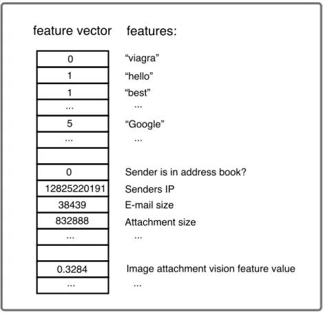
Consider an e-mail spam filtering application, where the goal is to build a classifier to predict if a new incoming e-mail is spam or not before delivering it to users’ inboxes. To build such a classifier, a large amount of training data is collected. In this example, the training data include e-mails (instances) and their corresponding labels as spam or not spam (outcomes). E-mail instances are formulated as quantitativefeature vectors readable by computers. Fea-tures may include words from the subject line and e-mail body, sending time, attachment types, attachment sizes in bytes, sender I.P., and spamming reputation. Figure 1.1 shows an example of the feature vector of one hypothetical e-mail instance.

A classifier is then learned to reproduce the outcome labels based on the instance features in the training data. The classifier determines which features to use and how to use them. A simple classifier might use the rule shown in Algorithm 1. This simple rule basically counts the number of occurrences of the keyword “viagra”, and checks if the sender is in the user’s

(15)

feature vector features: “viagra” “hello” “best” “Google”

Sender is in address book? Senders IP

E-mail size Attachment size

Image attachment vision feature value ... ... ... ... 0 1 1 5 ... ... ... ... 0 12825220191 38439 832888 0.3284

Figure 1.1: Features and the feature vector of one hypothetical e-mail instance. address book. If the occurrence is greater than one and the sender is a stranger, the e-mail is classified as spam.

After training, the learned classifier is applied to classify previously unseen e-mails, a process called test-time evaluation or testing. To classify a new e-mail, one has to convert a data instance (a new e-mail in raw input) to a quantitative feature vector like described above, in the format required by the classifier. This stage is called feature extraction. Once features are extracted and concatenated into a feature vector, the learned classifier performs some computation to generate final predictions. This stage is calledclassifier evaluation. Another simple example of classifier evaluation which executes a classifier prediction rule is shown in Algorithm 2. The rule assigns a weight to each feature, where the weight is learned during training. Then the rule sums the weighted features and if the sum exceeds a threshold, it is classified as spam and otherwise as non-spam.

(16)

Algorithm 1E-mail spam filtering rule 1

if (“viagra” _≥1) and (Sender is in address book == 0) then

return SPAM

else

return REGULAR

end if

Algorithm 2E-mail spam filtering rule 2

if 0.9_×“viagra” + 0.2_×“hello” _≥3 then

return SPAM

else

return REGULAR

end if

Performing feature extraction and classifier evaluation during testing is not free and each stage described above incurs some certain cost. Feature extraction cost reflects the computa-tional efforts of converting data instances to readable feature vectors. For example, counting the number of occurrences of keywords requires a full scan of the e-mail body, while extract-ing vision features from attached images requires runnextract-ing some vision algorithms. Classifier evaluation cost reflects the computation of generating predictions from feature vectors. For example, in Algorithm 2, the prediction rule requires multiply and sum operations, which consume CPU computation cost. These two costs combine to form test-time cost.

In the traditional machine learning setting, where data set sizes are small and classifiers are usually only executed once, test-time cost is low, and the sole goal is high classification accuracy. However, as machine learning enters into industry through applications such as web-search engines [142], product recommendation [40], and e-mail and web spam filter-ing [128], the settfilter-ing becomes different. In all these applications, data set sizes are very large and classifiers are executed millions of times everyday. The test-time cost becomes an equally important concern as accuracy. Imagine a classifier that is executed 10 million times per day. We would like to introduce a new feature that improves the accuracy by 3%, but its extraction increases the running time by 1s per execution. 10 million executions would require the project manager to purchase 58 days of additional CPU time per day. Imagine another example where in order to classify a new e-mail, a classifier has to compare the feature vector of the new e-mail against that of all training e-mails (e.g. 10 million e-mails). Introducing additional 10 million training e-mails improves the accuracy of the classifier by

(17)

1%, but also significantly increases the test-time evaluation cost, as the classifier evalua-tion cost is linear in the number of training inputs. From these two large-scale real-world applications, it is clear that the real-world industrial setting introduces a new problem to machine learning research: computational resources must be budgeted and costs must be strictly accounted for during test-time. At its core, this problem is an inherent trade-off

between accuracy and test-time cost.

In this thesis, we systematically investigate the test-time cost, quantify it, and propose four new approaches to explicitly control it under budget. To start, we first formally describe su-pervised learning and learning under test-time resource constraints. We then introduce some useful background in machine learning and give an overview of our four different approaches. In Chapter 2, we introduce two related algorithms that employ a strategy trading-off accuracy and test-time feature extraction cost. In Chapter 3 we describe another strategy, classifi-cation with trees and cascades, aiming to budget the amortized test-time cost. Chapter 4 targets the classifier evaluation cost and introduces an algorithm that explicitly controls it. Finally, Chapter 5 offers concluding remarks.

1.1 Learning and Learning Under Test-time Constraints

1.1.1 Supervised learning

Let xi ∈ X denote a training input in the form of a feature vector of dimension d, xi ∈ Rd_{, with label} _y

i ∈ Y. In supervised learning, training data are i.i.d. (independent and

identical distributed) samples from a joint distribution _D =_{X × Y} of instance/label pairs,

i.e. _{(x1, y1), . . . ,(xn, yn)}. Labels Y can be binary, categorical or real numbered. E-mail

spam filtering for example has binary labels, where each e-mail is either labeled as positive (regular) or negative (spam). Problems with binary, categorical and real number labels are referred to as binary classification, multi-class classification and regression problems, respectively.

Given the set of inputs and the corresponding labels, it is assumed that there is an underlying function f that maps the inputs to labels, yi = f(xi). The core of supervised learning is

(18)

to estimate this underlying function by learning an approximate hypothesis H _∈ _H from a large amount of training inputs and their labels, and this hypothesis H is called classifier. Typical supervised learning methods include Logistic regression [53] and Support Vector Machines (SVM) [110, 29] for classification problems, and Neural networks [55] and Kernel regression [84] for regression problems.

1.1.2 Supervised learning under test-time resource constraints

When learning under test-time resource constraints, there are a test-time budget B and a test-time costc. The test-time cost can be divided into feature extraction costcf and classifier

evaluation costce, corresponding to two stages during testing. A classifier’s intrinsic structure

(its prediction rule or algorithm) determines the evaluation cost, and thus the evaluation cost is a function of a specific classifierH,ce(H). We also assume that during testing, features are

extracted on-demand, where features are only extracted from data instances when needed by the classifier. Therefore, a classifier H determines which features to extract, and the extraction cost is also a function of a specific classifier, cf(H).

This test-time cost and budget dramatically transform supervised learning. Instead of just learning a classifier H to maximize classification accuracy, one should also take test-time cost and budget into consideration during learning, making sure that the test-time cost of a classifier will be within budget constraints, cf(H) +ce(H)≤B.

1.2 Types of Classifiers

Since a classifier’s intrinsic structure dramatically affects the test-time cost, we review dif-ferent types of classifiers. In general, a classifier H is learned by minimizing a loss function

` w.r.t. the classifier,

H = min

(19)

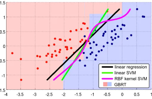
linear regression linear SVM RBF kernel SVM GBRT

Figure 1.2: Decision boundaries of linear regression, linear SVM, kernel SVM and GBRT. One example for ` is the squared-loss

`sq(H) = 1 2n n X i=1 (H(xi)−yi)2, (1.2)

but other losses, for example log-loss [53], are equally suitable.

1.2.1 Linear classifier

Linear classifiers have long been a popular classifier in statistics and machine learning, and still remain as an indispensable tool today. A linear classifier predicts an observed outcome

yi from a feature vector xi ∈ Rd using the model,

H(xi) =x>i w+b, (1.3)

where H(xi) is the prediction of the observed outcome yi, w ∈ Rd is the weight vector

(20)

decision boundary

margin

support vectors

Support Vector Machine (SVM)

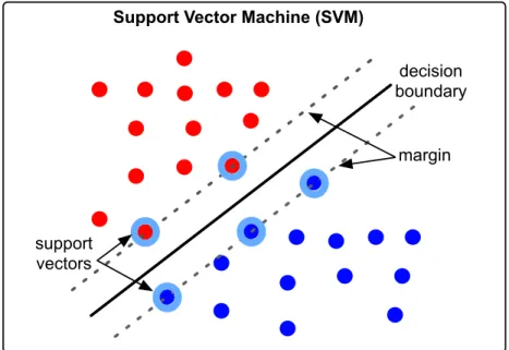
Figure 1.3: A schematic layout of Support Vector Machine (SVM). Blue and red dots are training instances in a two dimensional feature space, and two colors indicate two classes. The solid black line is the decision boundary learned from the training data. Dotted dark lines are margins. Dots in light blue circles are support vectors.

space, x, H(x)represents a hyperplane. This hyperplane is called a decision boundary for classification problems, as instances above the hyperplane are classified as positive and those below are classified negative. This decision boundary is parameterized by the weight vector

w, and it is learned by minimizing a squared-loss function

min w `(w) = n X i=1 (x>_i w+b₋yi)2. (1.4)

Figure 1.2 (black curve) shows a linear classifier and its decision boundary learned from a 2-dimensional Iris [2] data set. Commonly used linear classifiers include logistic regression and linear regression. In terms of the test-time cost, a linear classifier just needs to perform the inner product computation in (1.3), so the evaluation cost is very low.

(21)

1.2.2 Large margin classifier

To improve the generalization performance to previously unseen test data, Cortes and Vapnik [29] introduce Support Vector Machines (SVM). Compared to a regular linear model as described above, SVM enforces a large margin, maximizing the margin between the decision boundary and the closest training instances. Mathematically, the SVM decision boundary can be learned by solving an optimization problem:

min

w,b kwk (1.5)

s.t. yi(x>i w+b)≥1, i= 1, . . . , n,

where the objective function maximizes the margin, and the constraints enforce that the decision boundary is at least one unit away from training instances. One key advantage of the SVM is that its decision boundary is completely defined by training instances on the margin, denoted support vectors. Since the number of support vectors is usually less than training instances, SVM is also referred to as Sparse Vector Machine. Figure 1.3 illustrates the margin, decision boundary and support vectors. Figure 1.2 (green curve) shows the decision boundary of an SVM on the Iris data set. To make predictions, an SVM uses the prediction rule:

H(xi) = sign(x>i w+b). (1.6)

The test-time evaluation cost is the inner product computation and is very low.

1.2.3 Kernel classifier

While the large margin enforcement provides better generalization on unseen test data, it is still restricted by its linear decision boundary, and is unable to handle linearly un-separable data. To overcome this, Guyon et al. [52] propose kernel SVM. Kernel SVM allows the algorithm to find the maximum-margin hyperplane in a transformed feature space (x_→φ(x), where φ(x) _{∈ R}D, and D d). The transformation enlarges the feature space and may be nonlinear. Therefore, while the resulting decision boundary is still a linear hyperplane in the high-dimensional feature space, it may be nonlinear in the original input space. To learn

(22)

such a hyperplane, kernel SVM optimizes the following problem: min α1,...,αn 1 2 n X i=1 n X j=1 αiαjyiyjKij − n X i=1 αi, (1.7) s.t. n X i=1 αiyi = 0 and αi ≥0, i= 1, . . . , n,

whereα are the Lagrange multipliers [6], andK is the kernel matrix whose entryKij is the

inner product of the instances in the transformed space, Kij = φ(xi)>φ(xj). Compared to

other non-linear transformation [27, 107] the key advantage of this formulation is that one never needs to express φ(x) explicitly, instead using the kernel function Kij = k(xi,xj) to implicitly transform the feature space. Note that the above optimization is equivalent to (1.5), only expressed in dual form [6] with the implicit feature transformation φ(x).

The kernel SVM prediction function is different from linear SVM,

H(xi) = n X

j=1

αjyjKji+b, (1.8)

where Kji is one kernel entry, which is the value of a kernel function of a test input xi

and one support vector, Kji = k(xj,xi). Figure 1.2 (magenta curve) shows the non-linear

decision boundary of a kernel SVM. Since kernel SVM evaluation involves computing kernel function of a test input and all its support vectors, its classifier evaluation cost is significantly higher than linear classifiers. Other popular kernel classifiers include kernel regression [66] and Gaussian processes [98].

1.2.4 Tree-based classifier

Another set of classifiers are tree-based classifiers. They all use decision trees to partition the feature space into a set of rectangles, on which they train simple and weak classifiers. These weak classifiers are also referred to as weak learners. While conceptually simple, tree-based classifiers are powerful and produce non-linear decision boundaries. Popular tree-tree-based classifiers include random forest [8] and gradient boosted regression trees (GBRT)[44].

(23)

color = red Decision Tree

color red6=

radius < 2 radius 2 shape = round shape round6=

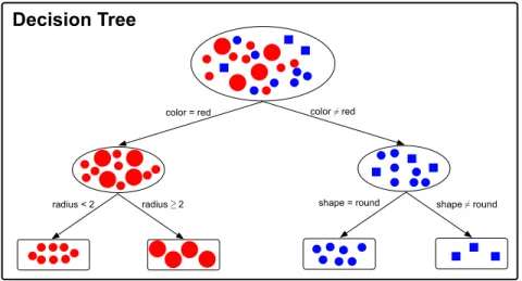
Figure 1.4: A schematic layout of a classification decision tree. Blue and red shapes are training instances in four classes (small red dot, large red dot, small blue dot and small blue rectangle). The black circles are decision tree internal nodes, and rectangles are leaf nodes. At each internal node, the decision tree partitions the input space by one of the features and a corresponding splitting value (e.g. radius <2). Leaf nodes make predictions based on the instances in each leaf.

Figure 1.4 illustrates a schematic layout of a classification decision tree. Blue and red shapes are training instances in four classes (small red dot, large red dot, small blue dot and small blue rectangle). The black circles are decision tree internal nodes, and rectangles are leaf nodes. At each internal node, the decision tree partitions the input space by one of the features and a corresponding splitting value (e.g. radius< 2). Leaf nodes make predictions based on the instances in each leaf.

In this thesis, we focus on GBRT, a tree-based ensemble classifier. Given a continuous and differentiable function `, GBRT learns an additive classifier,

H(x) =

m X

t=1

ηtht(x), (1.9)

whereH(x) minimizes the loss function,ht∈His one weak learner, andmis the total number

of weak learners. Specifically in GBRT, each ht is a limited depth regression tree [7] added

to the current classifier at iteration t, with learning rate ηt≥0. H is the set of all possible

regression trees of some limited depthb. LetHt−1denote the current predictor, the regression treehtis selected to minimize the function`(Ht−1+ηtht). This is achieved by approximating

(24)

the negative gradient of ` w.r.t. the current Ht−1, −_∂H_t₋∂`₁₍_x

i). The greedy classification

and regression tree (CART) algorithm [7] is often used to find the approximation. CART generates a limited-depth regression treeht∈ Hby greedily minimizing an impurity function,

g :_{H → R}+₀. Typical choices for g are the squared loss,

ht= argmin ht∈H X i − ∂` ∂Ht−1(xi) − ht(xi) 2 , (1.10)

but other losses such as label entropy [53] are equally suitable. CART minimizes the impurity function (1.10) by building a decision tree similar to Figure 1.4. Consequently, ht can be

obtained by supplying₋_∂H∂`

t−1(xi) as the regression targets for all inputsxi to an off-the-shelf

CART implementation [120].

To generate predictions, GBRT uses prediction function (1.9). During testing, a test instance traverses each decision tree. Because the decision trees are of limited depth, and each split is a simple threshold on single feature, the evaluation cost is relatively low. Figure 1.2 shows the decision boundary of GBRT. Red shaded area indicates positive prediction of GBRT and blue shaded area indicates negative prediction. The decision boundary is also non-linear.

1.2.5 Parametric vs. nonparametric

Classifiers described above can also be divided into two groups: parametric classifier and nonparametric classifier. Parametric classifiers have specific functional forms governed by a small number of parameters whose value are to be learned from data. For example a linear classifier is parameterized by the weight vector w. The important limitation of parametric model is that the chosen function might be a poor approximation to the true function that generates the observed data. In contrast, nonparametric classifiers make few assumptions about the form of the function. Instead, they treat training data as parameters and use them to make predictions. For example, a kernel regression classifier uses weighted outcomes of a test instance’s training neighbors to generate the prediction. Another way to distinguish parametric and nonparametric classifiers is by the relation of the number of parameters and training instance size. Parametric classifiers have a fixed number of parameters, independent to the training size, whereas the number of parameters of nonparametric classifiers grows

(25)

Parametric classifiers include linear regression, linear SVM and GBRT, and nonparametric classifiers include kernel regression, kernel SVM and random forest.

1.3 Motivation

Given that different classifiers have completely different intrinsic structures, their test-time cost is also vastly different. Therefore, we employ various strategies to deal with different learning scenarios. We first focus on the parametric classifiers, where the classifier evalua-tion cost is relatively low compared to the feature extracevalua-tion cost. Since features are often heterogeneous, extraction time for different features is highly variable. Which features to extract and how to balance the trade-off between accuracy and feature extraction cost be-comes a crucial problem. In this scenario, we employ a strategy that aims to reduce feature extraction cost.

GreedyMiser, described in Section 2.1, is a new algorithm that incorporates the feature extraction cost during training to explicitly minimize the CPU cost during testing. The algorithm proposes a novel impurity function to incorporate feature extraction cost and builds a connection to stage-wise regression (GBRT). The resulting classifier cherry-picks a few expensive expert features and many other good but inexpensive features to form a classifier, and greatly reduces the test-time cost.

We extend this strategy for reducing feature extraction cost to anytime classification, first introduced in [50]. Similar to the previous scenario, feature extraction cost dominates the time cost. However, unlike the previous scenario, in anytime classification, the test-time budget is explicitly unknown during training and testing. The classifier can be queried at any point to return the current best prediction. This may happen when the test-time budget is exhausted, the classifier is believed to be sufficiently accurate or the prediction is needed urgently (e.g. in time-sensitive applications such as pedestrian detection [47]). This unknown test-time budget introduces new problems, and we aim to learn a classifier that has a capability to produce accurate classifications at any possible budget.

Anytime Feature Representation Learning (AFR) [135], introduced in Section 2.2, describes a novel algorithm that explicitly addresses the problem of producing accurate classifications at

(26)

any budget. The algorithm lowers test-time feature extraction cost in the data representation rather than in the classifier. This enables us to turn conventional classifiers, in particular robust and accurate support vector machines (SVM), into test-time cost-sensitive anytime classifiers – combining the advantages of anytime learning and large-margin classification. We also budget the feature extraction cost from a different perspective. Instead of limiting the cost for all test inputs, we extract different features for different inputs, and aim to constrain the amortized cost. We propose the second strategy, classification with trees and cascades. Consider the e-mail spam filtering example. Some of the messages can be filtered out just based on their sender-IP address in less than one millisecond (possibly without even tokenizing the message content). Others can be detected by simple text features. Still other spam e-mails can be detected only by examining image attachments using vision features. Since different inputs can be correctly classified by a variety of features that are most beneficial, expensive features are only extracted to classify a few inputs, and thus the

amortized test-time cost can be reduced. Therefore, the goal is to construct a structured

classifier directing different inputs to different paths, so theamortized test-time cost is within the budget.

Cost-sensitive Tree of Classifiers (CSTC) [134] described in Chapter 3 covers a tree structured classifier that focuses on trading-off accuracy and amortized test-time feature extraction cost. It builds a tree of classifiers, through which test inputs traverse along individual paths. Each path extracts different features and is optimized for a specific sub-partition of the input space. By only computing features for inputs that benefit from them the most, the cost-sensitive tree of classifiers can match the high accuracies of the current state-of-the-art classifiers at a small fraction of the computational cost. It also has a natural extension, Cost-Sensitive Cascade of Classifiers (CSCC), which is designed specifically for binary classification tasks with high class imbalance.

Finally, we trade-off accuracy and nonparametric classifier evaluation cost using a model compression strategy. We focus on the scenario where the classifier evaluation cost is no longer trivial compared to feature extraction cost. For example, the learned model of a nonparametric classifier could be very large when training set is large, and thus the test-time evaluation cost is substantial. Note that this is very common in real-world applications, as their training input size could scale to millions. Therefore the evaluation cost has to be

(27)

budgeted and accounted for during test-time. The goal of model compression is to compress very large nonparametric models with an explicit objective of constraining their evaluation cost from running over the budget.

Compressed Vector Machines (CVM) introduced in Chapter 4 is a post-processing algorithm

thatcompresses the learned kernel support vector machine model by reducing and optimizing

support vectors. The algorithm cherry-picks a small subset of support vectors using least angle regression (LARS) [38], and then moves this subset of support vectors to match the decision boundary formed by the full model. Since computing the kernel function of testing inputs and support vectors dominates the evaluation cost, reducing the number of support vectors greatly reduces the cost. Moreover, the decision boundary formed by these moved

support vectors renders a relatively high prediction accuracy on testing inputs.

1.4 Some background in machine learning

In this section, we briefly discuss some useful background used throughout this thesis.

1.4.1 Boosting trick

Since the prediction function of gradient boosted regression trees (GBRT), H, is simply a linear function of each regression tree as in (1.9), regression trees can be interpreted as a non-linear transformation of the input data x_→h(x), where h(xi) = [h1(xi), . . . , hT(xi)]>,

ht ∈ H. H is the set of all possible regression trees of some limited depth b (e.g. b = 4)

and T = _|H|. We also denote β as the weight vector for transformed features, H(x) =

h(x)>β. The resulting feature space is extremely high dimensional and the weight-vector β is always kept to be correspondingly sparse. The above non-linear transformation is called the boosting-trick [44, 102, 22]. Because regression trees are negation closed (i.e. for each

h _{∈ H} we also have ₋h _{∈ H}) we assume throughout this thesis without loss of generality that β _≥ 0. Finally, we define a binary matrix F _{∈ {}0,1_}d×T _{in which an entry} _F

αt= 1 if

(28)

1.4.2 Gradient descent

Gradient descent is a numerical optimization method to find a local minimum of a function. It iteratively takes steps proportional to the negative of the gradient (or of the approximate gradient) of the function at the current point. Specifically, given a continuous and differen-tiable function f(x) and an initial guess x0 for a local minimum of f(·), gradient descent method goes from x0 in a direction of the negative gradient,−∂f_∂_x

x0 to a new point x1, x1 =x0 −η ∂f ∂x x0, (1.11)

where η is the learning rate. Gradient descent repeats this procedure and generates a se-quence of points such that

xd+1 =xd−ηd ∂f ∂x xd, d≥0. (1.12)

When ηd is small, the function value f(x) monotonically decreases along this sequence,

f(x0)_≥f(x1)_{≥ · · · ≥}f(xd) (1.13)

After certain iterations, the sequence (xd) converges to a local minimum. For convergence

proof, please see [6]. Note that the learning rate ηd can change at every iteration, and

searching for the optimal learning rate can be done through line search [6].

1.4.3 Conjugate gradient descent

We briefly discuss the Polack-Ribiere conjugate gradient descent method [95] used by several of our algorithms. Similar to gradient descent, conjugate gradient descent is also a numerical optimization method to find a local minimum of a function f(_·).

Figure 1.5 illustrates gradient descent (steepest descent) and conjugate gradient descent minimizing a quadratic function. The contours of the objective function are in gray scale, and the minimum is at the center represented by the darkest dot. Steepest descent (green arrows) takes many steps following the gradient direction. However, since it uses line search,

(29)

x0

x

_⇤ conjugate gradient descent steepest descent

Figure 1.5: A schematic comparison of conjugate gradient descent (red) and steepest descent with line search (green).

two consecutive gradient directions are always perpendicular to each other. Therefore, even when the function is a perfectly quadratic function, steepest descent repeatedly moves along the same directions.

In contrast, conjugate gradient descent searches the descent direction based on a quadratic approximation of the function,

f(x)_≈ 1 2x

>

Ax₋x>b+c. (1.14)

Given a positive definite matrixA, a pair of nonzero vectorspi,pj are conjugate if they are

orthogonal with respect to A,

p>_i Apj = 0. (1.15)

Since every pair of conjugate directions are linearly independent, a set ofdconjugate vectors spans the space in which the local minimumx∗ lies. Using conjugate directions, we iteratively

compute the next point using the update rule

xd+1 =xd−ηdpd, (1.16)

where pd is conjugate to all previous directions p0,· · · ,pd−1, and learning rate ηd is found

(30)

f(_·) at an initial guess point x0. In other words, p0 = ∂f_∂_x

x0. Polak [95] proves that at

iteration d(the dimension of the space in whichx∗ lies), the local minimum can be found by

conjugate gradient descent, xd= argminx∈Rdf(x). Figure 1.5 (red arrows) shows the steps

of conjugate gradient descent method. It finds the minimum with only two steps in this two dimensional space.

(31)

Chapter 2 Feature Extraction Cost Reduction

In this chapter, we focus on feature extraction cost and discuss two learning scenarios: low feature extraction cost classification and anytime classification, which employ a common strategy, reducing feature extraction cost. Section 2.1 discusses low feature extraction cost classification scenario and the proposed algorithm Greedy Miser. Section 2.2 discusses the second learning scenario, anytime classification and details Anytime Feature Representation

Learning (AFR).

2.1 Low Feature Extraction Cost Classification

Our proposed algorithm consists of many weak learners. Each weak learner is a limited depth regression tree boosted by a loss function. Different from gradient boosted regression trees (GBRT or stage-wise regression described in Section 1.2.4), our algorithm explicitly considers the test-time cost while boosting each weak learner, encouraging weak learners to cherry-pick good features and to re-use previously extracted features. We first state the (non-continuous) global objective which explicitly trades off feature extraction cost and accuracy, and relax it into a continuous loss function. Subsequently, we derive an update rule that shows the resulting loss lends itself naturally to greedy optimization with stage-wise regression [44]. Different from previous approaches [74, 105, 96, 24], our algorithm does not build cascades of classifiers. Instead, the cost/accuracy trade-off is pushed into the training and selection of the weak classifiers. The resulting learning algorithm is much simpler than any prior work, as it is a variant of regular stage-wise regression, and yet leads to superior test-time performance. We evaluate our algorithm’s efficacy on two real world data sets

(32)

from very different application domains: scene recognition in images and ranking of web-search documents. Its accuracy matches that of the unconstrained baseline (with unlimited resources) while achieving an order of magnitude reduction of test-time cost.

2.1.1 Related work

Previous work on learning under test-time resource constraints appears in the context of many different applications. Most prominently, Viola and Jones [125] greedily train a cas-cade of weak classifiers with Adaboost [108] for visual object recognition. Cambazoglu et al. [14] propose a cascade framework explicitly for web-search ranking. They learn a set of additive weak classifiers using gradient boosting, and remove data points during test-time using proximity scores. Although their algorithm requires almost no extra training cost, the improvement is typically limited. Lefakis and Fleuret [74] and Dundar and Bi [37] learn a soft-cascade, which re-weights inputs based on their probability of passing all stages. Differ-ent from our method, they employ a global probabilistic model, do not explicitly incorporate feature extraction costs and are restricted to binary classification problems. Saberian and Vasconcelos [105] also learn classifier cascades. In contrast to prior work, they learn all cas-cades levels simultaneously in a greedy fashion. Unlike our approach, all of these algorithms focus on learning of cascades and none explicitly focus on individual feature costs.

To consider the feature extraction cost, Gao and Koller [45] publish an algorithm to dy-namically extract features during test-time. Raykar et al. [99] learn classifier cascades, but they group features by their costs and restrict classifiers at each stage to only use a small subset. Pujara et al. [96] suggest the use of sampling to derive a cascade of classifiers with increasing cost for email spam filtering. Most recently, Chen et al. [24] introduce Cronus, which explicitly considers the feature extraction cost during training and constructs a cas-cade to encourage removal of unpromising data points early-on. At each stage, they optimize the coefficients of the weak classifiers to minimize the classification error and trees/features extraction costs. We pursue a very different (orthogonal) approach and do not optimize the cascade stages globally. Instead, we strictly incorporate the feature cost into the weak learners. Moreover, as our algorithm is a variant of stage-wise regression, it can operate naturally in both regression and multi-class classification scenarios.

(33)

−8 −6 −4 −2 0 2 4 6 8 −8 −6 −4 −2 0 2 4 6 8 −8 −6 −4 −2 0 2 4 6 8 −8 −6 −4 −2 0 2 4 6 8

Data Linear Kernel GBRT

−8 −6 −4 −2 0 2 4 6 8 −8 −6 −4 −2 0 2 4 6 8 −8 −6 −4 −2 0 2 4 6 8 −8 −6 −4 −2 0 2 4 6 8 (a) (b) (c) (d)

Figure 2.1: Gradient surface of a linear, a kernel and a GBRT classifier. (a) The linear un-separable simulation data. Red dots and blue dots are from two different classes, and the task is binary classification. (b) The gradient surface of a linear classifier, which is a hyper-plane (c) The gradient surface of a kernel classifier. (d) The gradient surface of a GBRT classifier.

2.1.2 Unique properties of stage-wise regression

In this subsection, we analyze the closely related algorithm of ours, stage-wise regression, and specifically, gradient boosted regression trees (GBRT) in detail. We give insights of some unique properties of GBRT that are desirable for learning under test-time resource constraints. We compare GBRT with a linear classifier and a kernel classifier. Let θ denote the parameters of a classifierH, and the goal of learning a classifier is to learn these param-eters θ by minimizing a loss function `. These parameters are usually learned by gradient descent, where at each iteration, we compute the gradient of the loss function ` w.r.t. the parameters, ∂`_∂θ. We apply the generalized chain rule, and decompose this gradient into two parts: ∂` ∂θ = n X i=1 ∂` ∂H(xi) ∂H(xi) ∂θ , (2.1)

whereH(xi) is the prediction of an inputxi. Note that the first part _∂H∂`₍_x

i) is the gradient of

the loss function` w.r.t. predicting function in function space evaluated at an input xi, and

the second part is the gradient of the predicting function w.r.t. its parameterθ. Compared to linear classifier and kernel classifier, there are two unique properties of GBRT: implicit parameterization and non-linear feature combination.

(34)

Implicit parameterization. Both linear classifier and kernel classifier have a predicting functionHthat can be represented as an analytical function of its parameters (i.e. for linear classifier, H(x) = x>θ, where θ_{∈ R}d_{). Therefore, when optimizing a linear or a kernel}

clas-sifier, one usually optimizes the classifier parameters directly through the gradient of the loss w.r.t. classifier parameters (i.e. _∂θ∂`). In contrast, there is no such an analytical function to model the predicting function H in GBRT. In other words, GBRT is parameterized implic-itly, and one has to learn the parameters of GBRT predicting function in two steps. Firstly, GBRT computes the negative gradient of the loss function w.r.t. predicting function in the function space _∂H∂`₍_x

i) evaluated at each input sample xi. Secondly, GBRT approximates this

negative gradient _∂H∂`₍_x

i) at every input xi by building a limited depth regression tree h(·)

using CART algorithm.

As described in section 1.2.4, CART generates a limited-depth regression tree ht ∈ H by

greedily minimizing an impurity function (1.10). It minimizes the impurity function by recursively splitting the data set on a single feature per tree-node. Note that features are only used when approximating the negative gradient in the CART algorithm, and therefore we can add constraints for feature extraction only in the CART algorithm. This provides more flexibility to incorporate structured feature information commonly used in computer vision, where the extraction of a feature from one vision descriptor (running one vision algorithm) sets all other features from the same descriptor free.

Non-linear feature combination. Different from linear classifiers, GBRT is capable of approximating a non-linear gradient surface. Shown in Figure 2.1 (a), we simulate a scenario where sample inputs are not linearly separable. Figure 2.1 (b-d) show the gradient surface

∂`

∂H of different classifiers. GBRT approximates the gradient surface through limited depth

decision trees. For a depth 4 tree, which has 24−1 = 8 leaf nodes, GBRT approximates the gradient surface by partitioning the space into 8 blocks (shown in (d)). Kernel classifier can also achieve non-linear approximation through kernel-trick, shown in (c). In contrast, a linear classifier is just a hyperplane in the input space (i.e. x>(∂`

∂θ)), which is shown in (b). The

key advantage of GBRT is that while it can achieve non-linear feature combination, it is still a parametric model. During test-time, parametric GBRT is much faster than nonparametric methods such as kernel SVM, and therefore is very suitable for large scaled data sets and test-time cost-sensitive applications.

(35)

2.1.3 Greedy Miser

In this subsection, we formalize the optimization problem of test-time computational cost, and then intuitively state our algorithm. We follow the setup introduced in [24], treating stage-wise regression classifier H as a linear combination of transformed feature spaceh(x) using boosting trick described in Section 1.4.1.

H(x) =h(x)>β, (2.2)

where β ∈ RT _{is the weight vector. We then formalize the test-time computational cost of}

the classifier H for a given weight-vector β.

Test-time computational cost. There are two factors that contribute to this cost: The function evaluation cost of all treesht withβt>0 (β is non-negative because the set of trees

is negation closed) and the feature extraction cost for all features that are used in these trees. Let e >0 be the cost to evaluate one tree ht if all features were previously extracted. Note

thateis a constant independent of the number of training sample inputs, and is usually very small if the tree depth is small. This is a key advantage of stage-wise regression over other nonparametric non-linear classifiers, as stage-wise regression is a parametric classifier. With this notation and the feature extraction cost cα and tree-feature indicator matrixFdefined

in Section 1.4.1, both costs can be expressed in a single function as

c(β) = e_kβ_k0+ d X α=1 cα T X t=1 Fαtβt 0 , (2.3)

where the l0-norm for scalars is defined as kak0 → {0,1} with kak0 = 1 if and only if

a ₆= 0. The first term captures the function-evaluation cost and the second term captures the feature costs of all used features. If we combine a loss `(β) with (2.3) we obtain our overall optimization problem:

min

β `(β), subject to: c(β)≤B, (2.4)

(36)

Algorithm. In the remainder of this section we derive an algorithm to approximately minimize (2.4). For better clarity, we first give an intuitive overview of the resulting method in this paragraph. Our algorithm is based on stage-wise regression, which learns an additive classifier Hβ(x) =

Pm

t=1βtht(x) that aims to minimize the loss function (2.4).1 During

iteration t, the CART algorithm is used to generate a new tree ht, which is added to the

classifierHβ.

Specifically, instead of using the regular impurity function (1.10), we propose an impurity function which on the one hand approximates the negative gradient of ` with the squared-loss, such that adding the resulting tree ht minimizes `, and on the other hand penalizes

the initial extraction of features by their costcα. To capture this initial extraction cost, we

define an auxiliary variable uα ∈ {0,1} indicating if feature α has already been extracted

(uα= 0) in previous trees, or not (uα= 1). We update the vector u after generating each

tree, setting the corresponding entry for used features α to uα:= 0. If we denote si as the

negative gradient, si =−_∂H∂`₍_x_i₎, our impurity function in iteration t becomes

g(ht) = 1 2 X i (si−ht(xi))2+λ d X α=1 uαcαFαt, (2.5)

where λ trades off the loss with the cost.

To combine the trees ht into a final classifier Hβ, our algorithm follows the steps of regular

stage-wise regression with a fixed step-size η >0. As our algorithm is based on a greedy

optimiser, and is stingy with respect to feature-extraction, we refer to it as the Greedy

Miser. Algorithm (3) shows a pseudo-code implementation.

Algorithm Derivation

In this subsection, we derive a connection between (2.4) and our Greedy Miser algorithm by showing that Greedy Miser approximately solves a relaxed version of the optimization problem.

1_{Here, without loss of generality. the trees in}

Hare conveniently re-ordered such that exactly the firstm

(37)

Algorithm 3Greedy Miser in pseudo-code

Require: D=_{(xi, yi)}ni=1, step-size η, iterations m

H= 0

for t= 1 to m do

ht ←Use CART to greedily minimize (2.5).

H _←H+ηht.

For each feature α used in ht, set uα←0. end for

ReturnH

Relaxation. The optimization as stated in eq. (2.4) is non-continuous, because of the l0 -norm in the cost term—and hard to optimize. We start by introducing minor relaxations to both terms in (2.3) to make it better behaved.

Assumptions. Our optimization algorithm (for details see subsectionOptimization on page 25) performs coordinate descent and — starting fromβ=0 — increments one dimension of βbyη >0 in each iteration. Because of the extremely high dimensionality (which is dictated by the number of all possible regression trees that can be represented within the accuracy of the computer) and the comparably tiny number of iterations (_≤5000) it is reasonable to assume that one dimension is never incremented twice. In other words, the weight vector β is extremely sparse and (up to re-scaling by 1_η) binary: 1_ηβ _{∈ {}0,1_}T_.

Tree-evaluation cost. Thel0-norm is often relaxed into the convex and continuousl1-norm. In our scenario, this is particularly attractive, because if 1_ηβ is binary, then the re-scaled l1 norm is identical to the l0 norm—and the relaxation is exact. We use this approach for the first term:

e_kβk0 −→

e

ηkβk1. (2.6)

Feature extraction cost. In the case of the feature cost, l1-norm is not a good approxi-mation of the original l0-norm, because features are re-used many times, in different trees. Usingl1-norm would imply that features that are used more often would be penalized more than features that are only used once. This contradicts our assumption that features become

(38)

We therefore define a new function _{k · k}d1, which is a re-scaled and amputated version of the l1-norm: kx_kd1 = ( |x η| for |x| ∈[0, η) 1 for _|x_{| ∈}[η,_∞). (2.7)

This penalty function _{k · k}d1 behaves like the regular l1 norm when |x| is small, but is capped to a constant when _|x_{| ≥} η. Note that while we use the notation _{k · k}d1 for the amputated version of the l1-norm, it is not a well-defined norm, as it is not homogeneous (_ktx_kd1 6=tkxkd1) With this definition, our relaxation of the feature-cost term becomes:

d X α=1 cα T X t=1 Fαtβt 0 −→ d X α=1 cα T X t=1 Fαtβt _d 1 . (2.8)

Similar to the previous case, if 1_ηβ is binary, this relaxation is exact. This holds because in (2.8) all arguments of_k·kd1 are non-negative multiples ofη(asFαt∈{0,1}andβt∈{0, η})

and it is easy to see from the definition of _{k · k}d1 that for allk = 0,1, . . ., we have kkηkd1 = kkη_k0.

Continuous cost-term. To simplify the optimization, we split the budget into two terms

B =Be+Bf—the tree-evaluation budget and the feature extraction budget—and re-write

(2.4) with the two penalties (2.6) and (2.8) as two individual constraints. If we use the Lagrangian formulation [6], with Lagrange multiplier λ (up to re-scaling), for the feature cost constraint and the explicit constraint formulation for the tree-evaluation cost, we obtain our final optimization problem:

min β `(β) +λ d X α=1 cα X t Fαtβt _d 1 (2.9) s.t. e ηkβk1 ≤Be. Optimization

In this subsection we describe how Greedy Miser, our adaptation of stage-wise regression [44], finds a (local) solution to the optimization problem in (2.9).

(39)

Solution path. We follow the approach from [102] and find a solution path for (2.9) for evenly spaced tree-evaluation budgets, ranging from B_e0= 0 to B_e0 =Be. Along the path we

iteratively increment B0_e by η. We repeatedly solve the intermediate optimization problem by warm-starting (2.9) with the previous solution and allowing the weight vector to change byη, min δ≥0 L(β+δ) z }| { `(β+δ) +λ d X α=1 cα X t Fαt(βt+δt) _d 1 , (2.10) s.t. _kδk1 ≤η.

Each iteration, we update the weight vector β :=β+δ.

Taylor approximation. The Taylor expansion of _L is defined as

L(β+δ) = _L(β) +_h∇L(β),δi+O(δ2). (2.11) If η is sufficiently small2, and because _|δ| ≤η, we can use the dominating linear term in (2.11) to approximate the optimization in (2.10) as

min

δ≥0h∇L(β),δi, s.t. kδk1 ≤η. (2.12)

Coordinate descent. The optimization (2.12) can be reduced to identifying the direction of steepest descent. Let _∇L(β)t denote the gradient w.r.t. the tth dimension, and let us

define

t∗ = argmin

t ∇L(β)t, (2.13)

to be the gradient dimension of steepest descent. Because _H is negation closed, we have ∇L(β)t∗ = −k∇L(β)k_∞. (If ∇L(β)_t∗= 0 we are done, so we focus on the case when it is

<0). With H¨older’s inequality we can derive the following lower bound of the inner product 2_{Please note that we see this as a true approximation, and do not expect}_η _{to be infinitesimally small—} which would cause the number of steps (and therefore trees) to become too large for practical use.

(40)

in (2.12),

h∇`(β),δi ≥ −|h∇L(β),δi| ≥ −k∇L(β)_k∞kδk1

≥η_∇L(β)t∗. (2.14)

We can now construct a vector δ∗ _{for which (2.14) holds as} _equality_{, which implies that}

it must be the optimal solution to (2.12). This is the case if we set δ_t∗∗ =η and δ₆₌∗_t∗= 0.

Consequently, we can find the solution path with steepest coordinate descent under step-size

η.

Gradient derivation. The gradient _∇L(β)t consists of two parts, the gradient of the

loss ` and the gradient of the feature-cost term. For the latter, we need the gradient of kPtFαtβtkd1, which, according to its definition in (2.7), is not well-defined if

P

tFαtβt=η.

As our optimization algorithm can only increase βt, we derive this gradient from the right,

yielding ∇ X t Fαtβt d1 = ( ₁ ηFαt | P tFαtβt|< η 0 _|P_tFαtβt| ≥η. (2.15)

Note that the condition_|P_tFαtβt|< η is true if and only if feature αis not used in any trees

with βt>0. Let us define uα = {0,1} with uα = 1 if and only if | P

tFαtβt|< η. We can

then express the gradient of _L (with a slight abuse of notation) as

∇L(β)t := ∂` ∂βt + λ η d X α=1 cαuαFαt. (2.16)

Applying the chain rule, we can decompose the first term in (2.16), _∂β∂`

t, into two parts: the

derivatives w.r.t. the current prediction Hβ(xi), and the partial derivatives of Hβ(xi) w.r.t.

βt. This results in ∇L(β)t= n X i=1 ∂` ∂Hβ(xi) ∂Hβ(xi) ∂βt +λ η d X α=1 cαuαFαt. (2.17)

(41)

As Hβ(xi) =h(xi)>β is linear, we have

∂Hβ(xi)

∂βt =ht(xi). If we define si = −

∂`

∂Hβ(xi), which

we can easily compute for every xi, we can re-phrase (2.17) as

∇L(β)t= n X i=1 −siht(xi) + λ η d X α=1 cαuαFαt. (2.18)

The Greedy Miser. For simplicity, we restrict _H to only normalized regression-trees (i.e. P

ih2t(xi) = 1), which allows us to add two constant terms 1₂ P

ih2t(xi) and 1₂ P

is2i to (2.18)

without affecting the outcome of the minimization in (2.13), as both are independent of t. This completes the binomial equation and we obtain a quadratic form:

ht= argmin ht∈H 1 2 n X i (si−ht(xi))2+λ0 d X α=1 cαuαFαt, (2.19)

with λ0 = λ_η. Note that (2.19) is exactly what Greedy Miser minimizes in (2.5), which concludes our derivation.

Meta-parameters. The meta-parameters of Greedy Miser are surprisingly intuitive. The maximum number of iterations, m, is tightly linked to the tree-evaluation budgetBe. The

optimal solution of (2.12) must satisfy the equality _kδ∗_k

1=η (unless∇L=0, in which case a local minimum has been reached and the algorithm would terminate). As_kβk1 is exactly increased byη in each iteration, it can be expressed in terms of the number of iterationsmof the algorithm, and we obtain 1_η_kβ_k1 =m. Consequently, in order to satisfy thel1 constraint in (2.9), we must limit to the number of iterations tom _≤ Be

e . The parameterλ

0 _corresponds

directly to the feature-budget Bf. The algorithm is not particularly sensitive to the exact

step-sizeη, and throughout the results section we set it toη= 0.1.

2.1.4 Results

We conduct experiments on two learning under test-time resource constraints benchmark tasks from very different domains: the Yahoo Learning to Rank Challenge data set [18] and the scene recognition data set from [71].

(42)

0 0.5 1 1.5 0.61 0.62 0.63 0.64 0.65 0.66 0.67 0.68 0.69 0.7

Stage−wise regression (Friedman, 2001) Stage−wise regression feature subsets Early exit (Cambazoglu et. al. 2010) Cronus optimized (Chen et. al. 2012) Greedy Miser 0 0.5 1 1.5 2 x 104 0.58 0.6 0.62 0.64 0.66 0.68 0.7

Stage−wise regression = 0 Greedy Miser = 0.5 Greedy Miser = 1 Greedy Miser = 2 Greedy Miser = 4 Greedy Miser

Test-time cost (large Yahoo set) Test-time cost (small Yahoo set)

N D CG @ 5 N D CG @ 5

Cost / test-accuracy tradeoff Test-accuracy under increasing iterations

⇥104 ⇥104 =1 4 =1 16 = 0 = 1 = 4

Figure 2.2: The NDCG@5 and the test-time cost of various classifier settings. Left: The comparison of the original Stage-wise regression (λ = 0) and Greedy Miser under various feature-cost/accuracy trade-off settings (λ) on the full Yahoo set. The dashed lines represent the NDCG@5 as trees are added to the classifier. The red circles indicate the best scoring iteration on the validation data set. Right: Comparisons with prior work on test-time optimized cascades on the small Yahoo set. The cost-efficiency curve of Greedy Miser is consistently above prior work, reducing the cost, at similar ranking accuracy, by a factor of 10.

Yahoo Learning to Rank. The Yahoo data set contains document/query pairs with label values from_{0,1,2,3,4_}, where 0 means the document is irrelevant to the query, and 4 means highly relevant. In total, it has 473134, 71083, 165660, training, validation, and testing pairs. As this is a regression task, we use the squared-loss as our loss function`. Although the data set is representative for a web-search ranking training data set, in a real world test setting, there are many more irrelevant data points. Usually, for each query, only a few documents are relevant, and the other hundreds of thousands are completely irrelevant. Therefore, we follow the convention of [24] and replicate each irrelevant data point (label value is 0) 10 times.

Each feature in the data set has an acquisition cost. The feature costs are discrete values in the set _{1,5,10,20,50,100,150_}. The unit of these costs is approximately the time to evaluate a tree ht(·). The cheapest features (cost value is 1) are those that can be acquired

by looking up a table (such as the statistics of a given document), whereas the most expensive ones (such as BM25F-SD described in [9]), typically involve term proximity scoring.

Supervised Machine Learning Under Test-Time Resource Constraints: A Trade-off Between Accuracy and Cost

Washington University in St. Louis

Washington University Open Scholarship

Supervised Machine Learning Under Test-Time

Resource Constraints: A Trade-off Between

Accuracy and Cost

Zhixiang Xu

c

Contents

List of Figures

List of Tables

Acknowledgments

Zhixiang (Eddie) Xu

Chapter 1

Introduction

1.1

Learning and Learning Under Test-time Constraints

1.1.1

Supervised learning

1.1.2

Supervised learning under test-time resource constraints

1.2

Types of Classifiers

1.2.1

Linear classifier

1.2.2

Large margin classifier

1.2.3

Kernel classifier

1.2.4

Tree-based classifier

1.2.5

Parametric vs. nonparametric

1.3

Motivation

1.4

Some background in machine learning

1.4.1

Boosting trick

1.4.2

Gradient descent

1.4.3

Conjugate gradient descent

x0

x

Chapter 2

Feature Extraction Cost Reduction

2.1

Low Feature Extraction Cost Classification

2.1.1

Related work

2.1.2

Unique properties of stage-wise regression

2.1.3

Greedy Miser

2.1.4

Results