Porametr Leegomonchai North Carolina State University Raleigh, NC and

∗

Porametr Leegomonchai

North Carolina State University

Raleigh, NC 27695-8110

pleegom@unity.ncsu.edu

and

Tomislav Vukina

North Carolina State University

Raleigh, NC 27695-8109

tom_vukina@ncsu.edu

Preliminary Version, May 2002

Please do not cite or quote or distribute without prior permission.

∗ _{This research has been partially supported by the USDA, Grain Inspection, Packers and Stockyards}

Administration through the cooperative agreement No. 99-ESS-02. All opinions expressed in the paper are those of the authors and not of the USDA, GIPSA.

Abstract

The objective of this paper is to test whether broiler integrators, after observing their contract growers’ abilities in the sequences of repeated short-term contracts, systematically discriminate among growers by strategically distributing production inputs of varying quality. The discrimination can either take the form of providing high ability agents with high-quality inputs or providing low ability agents with high quality inputs. The first integrator’s strategy would stimulate the career concerns type of response on the part of the growers, whereas the second strategy would generate a ratchet effect. We test this hypothesis by using the broiler contract production data. The result detects no discrimination in the provision of inputs by the integrator. We interpret the results to mean that both career concerns and ratchet effect hypotheses are simultaneously rejected.

1. Introduction

In many business environments, including agriculture, economic agents often contract with each other repeatedly. Ideally such relationships are governed by extensive long-term contracts. If two parties can sign a complete long-term contract, they can always contractually duplicate how they would behave in the absence of such contracts and in general do better (Laffont and Tirole, 1993). In practice, however, business is often conduced by a series of short-term contracts due to the unwillingness or inability of parties to commit to a long-term relationship. Commitment refers to the ability of economic agents to restrict their future actions in advance by pledging to stick to the contract until some predetermined date (Salanie, 1997, p.144). There are various reasons for the lack of commitment depending on the institutions considered. For example, regulators may not be able to commit because of the legal and political prohibitions on long-term commitment. Firms may be reluctant to enter fixed long-term contracts due to the uncertain market environment in which they operate. In most cases the lack of information necessary to contractually describe future technologies and environments may render current long-term contract meaningless in the future.

In dynamic contracts, the lack of commitment is the source of implicit incentives, which can be either perverse (negative) or positive. Implicit incentives arise when a principal has some ex post capacity to respond to an agent’s performance and when the agent’s current performance is informative about his future performance (Meyer, 1995). The best known implicit incentive is the “ratchet effect” which arises in situations when the employer cannot commit not to revise an employee’s compensation holding him to a higher standard tomorrow as a result of his good performance today. The same incentive problem arises for a regulated firm that may not want to produce efficiently today fearing the regulator might infer that low cost production is easy to achieve and impose even tighter constraints in the future. Positive implicit incentives are reputation and career concerns. Managers in firms, for example, may be motivated not only by the explicit contractual links between pay and performance but also because good performance today will enhance the labor market’s perception of one’s ability and hence improve future earnings (Meyer and Vickers, 1997; Holmstrom, 1999).

An interesting characteristic of many agricultural contracts such as for example livestock contracts is that they are always explicitly uniform and short-term. This means that all agents contracting with the same principal are operating under formally identical contract provisions and contracts cover only one flock or one batch at a time (Levy and Vukina, 2002). In dynamic incentive problems such as repeated production contracts, unless the principal can fully commit not to change the contract provisions for the entire duration of the relationship, in which case a dynamic incentive problem becomes essentially static, implicit incentives are potentially important even when explicit incentives can be provided. This is because the current performance affects not only the current reward, but may also affect the terms of the future explicit or implicit incentive contract.

The existence of a uniform short-term contract does not necessary mean that all agents are treated equally. When the principal and agents contract repeatedly, an explicitly uniform contract leaves the possibility to the principal to treat agents differently after learning about their abilities over time. For example, the principal may assign more difficult tasks to higher-abilities agents or may strategically distribute variable quality inputs such that they end up in the hands of agents who can make the best use of them.

Depending on the production technology, such discrimination of agents can cause hidden incentives of either negative (ratchet effect) or positive (career concerns) type. In fact, the complaints of contract broiler growers that they have been treated unfairly at the hands of processors have been well documented by Tsoulouhas and Vukina (2001) and Lewin-Solomon (2000). One of the arguments frequently raised was that the settlements of these contracts are biased because the initial quality and distribution of production inputs are exclusively under control of the principal.

The objective of this paper is to test whether broiler processors, called integrators, after observing their contract growers’ abilities in the sequences of repeated short-term contracts systematically discriminate among growers by strategically distributing production inputs of varying quality. The discrimination can either take the form of a strategy that provides high ability agents with high-quality inputs or an alternative strategy to provide low ability agents with high quality inputs. The first integrator’s strategy would stimulate the career concerns type of response on the part of the growers, whereas the second strategy would generate a ratchet effect type of response. The type of discrimination that will occur depends on the technological characteristics of the broiler production process. Available survey data and overwhelming anecdotal evidence suggest that the career concerns type of response is more likely.

The ratchet effect was first recorded in the comparative economic systems literature (Berliner, 1957) citing empirical evidence from the Soviet Union that showed that planners would often penalize plant managers for the increased output under new incentive schemes, claiming the higher output proved shirking in the earlier period. The subsequent literature on ratchet effect is mainly found within the theoretical research on the dynamics of complete contracts with no commitment. Weitzman (1980) has analyzed the behavior of a regulated firm facing an incentive scheme that moves according to some exogenous, backward looking revision rule. One of the first game-theoretic analyses of the ratchet effect is Yao (1988) who considered a two-period model of emission standard setting by the EPA. Probably the most known piece is Freixas, Guesnerie and Tirole (1985) who explore the ratchet effect under the assumption that the planner cannot commit to a revision procedure which leads to excessive pooling equilibria. Despite the substantial theoretical attention that has been given to the ratchet effect, models that

include them have not been empirically tested against contract data. To the best of our knowledge the only exception is Allen and Lueck (1999) who studied crop share and cash-rent land contracts and found no evidence of the economically important ratchet effect.

In the theoretical part of the paper we model the optimal grower response in the full commitment (static) and no-commitment (dynamic) environments. Our approach is based on the passive target setting revision rule similar to Weitzman (1980). The empirical analysis is carried out using the contract production data for broiler chickens. Our econometric model specifies the quality of production inputs received by a grower as a function of his abilities. We measure grower ability as the historical deviation from the average settlement cost. The quality of production inputs is measured by the quality of one-day old chicks and the quality of chicks is approximated by the age of laying hens. The results show that there is no significant input discrimination among growers based on their abilities. We believe that the results can be interpreted as the simultaneous rejection of both career concerns and ratchet effect hypotheses.

2.The Broiler Industry

The broiler industry is often considered a role model for the industrialization of agriculture. The industry is entirely vertically integrated from breeding flocks and hatcheries to feed mills, transportation divisions and finally processing plants. A large proportion of the industry value added comes from the processing stage, which explains why the processors became the coordinators of the industry. The finishing stage (the final stage of the production process where one-day-old chicks are brought to the farm and grown to market weight) is organized almost entirely through contracts between processors and independent growers. Broiler contract production is dominated by large national companies such as Perdue and Tyson, which run their operations through smaller profit centers spread throughout the country.

Modern broiler production contracts are agreements between an integrator and growers that bind growers to tend for company’s chickens until they reach market weight by strictly following specific production practices in exchange for monetary compensation. All profit centers offer identical contracts to all prospective growers on a take-it-or-leave-it basis. Contracts have two main components: one is the division of

responsibility for providing inputs, and the other is the use of tournaments to determine grower compensation. Broiler production contracts require growers to construct and equip the chicken houses; they are also responsible for supplying labor, utilities, maintenance, and some other smaller items. The integrator’s responsibility is to provide baby chicks, feed, medication and the services of the field personnel (Vukina, 2001).

Most of the modern broiler contracts are settled using a two-part piece-rate tournament consisting of a fixed base payment per pound of live meat produced and a variable bonus payment based on the grower's relative performance. The bonus payment, usually called “the adjusted prime cost rating” is calculated as a percentage of the difference between group average settlement costs and grower’s individual settlement costs. Settlement costs for each grower are calculated by adding chicks, feed, fuel, medication, and other flock costs divided by total pounds of live broiler produced. The calculation of the group average settlement costs includes growers whose flocks were harvested within the same week. For the below average settlement costs, the grower receives a bonus, for the above average settlement costs, he receives a penalty. The number of growers in the settlement group varies in the 10-35 range depending on the size of the integrator as well as other logistical and market conditions. Specifically, the payment to grower k for flock t is calculated as:

kt j kt kt jt jt t t k Y Y c Y c n r D I R                 − − + = 1

∑

,

where I is the base payment, U ∈[0,1] is the slope of the payment scheme that determines

the relative importance of the bonus payment in the total grower’s compensation, Ykt is the number of live pounds of broilers produced, c is the cost of inputs supplied by the _kt

integrator to grower k (chicks, feed, medication, etc.),

∑

j jt jt Y c n 1

is the flock average per

pound settlement cost, and Dt is the market price adjustment specified as the percentage difference between the market price for broilers and the integrator’s average variable production costs.1

1

The market price clause “M” is a relatively new modification to a standard broiler tournament contract and does not exist in all contracts.

An interesting feature of the broiler contracts is that they are short-term, i.e., they cover one flock at a time. Contracts generally do not guarantee to the growers a fixed number of flocks per year, hence the decision about the volume of production (rotation of flocks on a farm) is determined solely by the integrator. This flexibility is important to the integrators because by delaying the delivery of new flocks to growers they can manipulate their total supplies in response to the market signals. In most instances, after one flock is harvested the contract gets tacitly renewed and the grower receives a new flock. The cases of grower terminations are extremely rare and are typically caused by a major violation of the contract stipulations (e.g. gross negligence or theft of feed or birds) or by the closure of a profit center or the bankruptcy of the company. It is not unusual for the contract growers to spend their entire career growing chickens for one integrator. Therefore, over time, the integrator can develop a precise knowledge of growers’ abilities. However, the explicit contracts almost never change despite the fact that the integrators may be able to benefit from offering different contracts to different types of growers.

2.1. Distribution of Inputs

Aside from the standard moral hazard type of problems associated with growers’ effort being unobservable by the integrator, from the perspective of this study the asymmetry of information regarding the provision of integrator’s inputs is particularly important. For example, growers usually observe only the quantity of inputs they receive at the time of delivery but not the quality of inputs. The quality will be revealed to them only after the production process is completed and the results are compared against other growers in the same tournament and against historical averages of previous flocks. The growers’ complaints about the provision of inputs have well been documented in trade magazines and academic literature. For example, an industry survey conducted by Ilvento and Watson (1998) reveals that approximately 40% of the growers feel that the quality of chicks is not evenly distributed among growers and 50% are doubtful about the fairness of the process. About 40% of growers questioned the matching of the feed weight tickets and the actual feed deliveries to the farms, whereas several growers feel that good-quality chicks are consistently delivered to the newer broiler houses. The quotes of several representative complaints from the survey are as follows:

“We have no control over quality of feed or chicks.” (p.58)

“A competitive contract is unfair, too many things not in control of grower such as vaccines, chick quality, flock experiments; some flocks convert, some do not.” (p.56)

“Bad chicks, time of day chickens are delivered, error in feed delivered, etc., makes the pay a lot different than other growers with no bad birds.” (p.56)

These and similar complaints may be well founded. Because the written contracts specify no commitment from the integrator regarding the fair distribution of inputs, having information about growers’ abilities the integrator may discriminate among them by strategically distributing uneven quality inputs to minimize cost of production. The variation in the quality of inputs can be significant, especially when it comes to baby chicks and feed. There are two possible technological scenarios that the integrator can exploit. The first scenario is to give high-quality inputs to high-ability growers and low-quality inputs to low-ability growers. We call this scenario “Technology A”. The second scenario is to give high-quality inputs to low-ability growers and low-quality inputs to high-ability growers. We call this scenario “Technology B”. Which scenario are we more likely to observe depends, of course, on which one of them yields lower unit cost of production.

As an illustration, let’s assume that we have two levels of quality of inputs (xH =high quality and xL =low quality) and two growers (grower L is assumed to be

more able than grower j). The integrator will implement technology A if the marginal product of high-ability grower is larger than that of a low-ability grower when both are using the high-quality inputs, whereas the marginal products of both using the

low-quality inputs are approximately equal. Mathematically,

H j H i x y x y ∂ ∂ > ∂ ∂ and L j L i x y x y ∂ ∂ ≈ ∂ ∂ ,

where y and _i y denote outputs from grower _j L and M respectively. In other words, the

integrator will implement technology A if she knows that the high ability growers can utilize the high quality inputs more effectively than the low ability growers, whereas their performances when both of them use the low quality input are indistinguishable. Technology B will be adopted if the marginal products from utilizing the high-quality input are approximately the same for both types and the high-ability growers can utilize

low-quality inputs more efficiently than the low-ability growers ( H j H i x y x y ∂ ∂ ≈ ∂ ∂ and L j L i x y x y ∂ ∂ > ∂ ∂

). This can happen if the integrator believes that high ability growers may

somehow salvage low quality chicks from performing really poorly, whereas the good quality chicks will perform well no matter who tends for them.

Based on Ilvento and Watson (1998), we have more reasons to believe that Technology A more accurately describes the intricacies of efficient broiler production than Technology B. In many responses one can find strong evidence that growers feel that if they received low quality chicks they are behind in the tournament from the start because those chicks are simply non-performing. Even the best among growers cannot do anything with lousy inputs. The quotes listed below illustrate this point:

“(Growers) can take the best (chicks) and make them worst, but growers cannot take the worst (chicks) and make them best.” (p.60)

“Garbage (chicks) in, garbage out.” (p.55)

“ If you get bad chicks (they know before you get them), it doesn’t do any good what you or they do. They are going to be bad.” (p.68)

In summary, the integrator who is a tournament organizer will update her beliefs about each grower’s abilities based on the settlement costs in repeated tournaments and absent significant transaction costs will have incentives to strategically distribute inputs to growers according to their types. If Technology A is the integrator’s cost minimizing strategy, this should create a career concerns type of dynamic incentives for the growers because doing well in the current tournament has double benefits. When a grower manages to produce broilers at below average settlement cost, he will not only earn the current period bonus but will also improve his chances of receiving high quality inputs in the next period tournament. Contrary to this, Technology B should generate a ratchet effect type of dynamic incentives. This is because the benefits of doing well in the current tournament (thereby signaling one’s high ability) are to a certain degree offset by an increasing chances of being stuck with the low quality input in the next period tournament. In the next section we model growers’ dynamic incentives more precisely.

3. Model

The production of broiler chickens is organized via short-term (one flock at a time) contracts and the payment is based on a piece-rate (cardinal) tournament. Prior to the beginning of production, the integrator offers an identical contract to all growers. For simplicity, we assume that in each tournament the competition takes place only between two growers, k =i,j, randomly drawn from the population of n growers that grow chickens for that integrator. We also assume that the contract will be automatically renewed for one more flock, such that the total number of time periods (flocks) in our model is two, t = 1,2. The payment scheme is of the following form

)

( _{kt kt}

kt I r y y

R = + − ₋ (1)

where R is the payment to grower k in period t, kt I is the base payment, U is the slope of

the bonus payment and y is the level of output. The bonus payment is determined as a _kt

percentage of the difference between growers’ output levels.2 It is obvious that the aggregate bonus payment is a wash, that is, the winner’s bonus will exactly cancel the loser’s penalty and the total integrator’s compensation expenditure in a given tournament is only 2×I.

Growers are assumed to be risk neutral with identical utility functions ))

, ( (Rkt C ekt k

U − θ , where C(ekt,θk)is the cost (disutility) of effort that depends on effort and the grower’s type. The difference between the high ability type and low ability type is reflected in the cost of effort such that C(e_kt,θ =_k) θ_ke_kt2 2where θ <_i θ_j means that grower i is of higher ability than grower j. To simplify we choose θ_i =1and θ_j >1. The exertion of effort e_kt∈[ e0, ] is essential for the cost to exist, C(e_kt =0,θ_k)=0; cost is

2

Notice that the payment mechanism that we use is a somewhat simplified version of the actual scheme described in Section 2. The main difference comes from our assumption that the total quantity of inputs delivered is fixed and the competition among growers is about producing more output (heavier birds). Other studies dealing with broiler tournaments (e.g. Knoeber and Thurman, 1994 and Tsoulouhas and Vukina, 1999) have assumed that the output is fixed and that the growers compete for better feed efficiency. The latter approach implicitly assumes constant percentage mortality across all growers, whereas this study assumes constant feed utilization across all growers, both of which are to a certain extent simplifications of reality.

increasing in effort, >0 ∂ ∂ kt e C

; and the more able the grower, the lower his marginal cost

of effort, 0 2 > ∂ ∂ ∂ k kt e C θ . 3

Suppose now that the production of broilers is a function of the fixed quantity of inputs provided by the integrator to each grower X and the grower’s effort _kt HNW . For

simplicity, we assume that half of the integrator’s inputs is of high quality, xH, and the

remaining half is of low quality, xL. One of the two growers receives q fraction of t xH

and (1−q_t) of x_L and the other grower of course receives (1−q_t)of [+ and q of t xL.

More specifically, the production function for grower i can be represented by the

following stochastic technology

it t it L it H it it q x q x e u y =( +(1− ) ) + +ξ (2)

where XWis the common production shock and ξW is an individual grower’s idiosyncratic

shocks. Both shocks are iid with mean zero and finite variance.

In the rest of the model section we will stick with the assumption that correct description of the efficient production process is embedded in Technology A

characterized by H j H i x y x y ∂ ∂ > ∂ ∂ and L j L i x y x y ∂ ∂ = ∂ ∂

. It is easy to show that the results with

Technology B are mirror images of the results based on Technology A. The assumption that the marginal productivity of low quality input is invariant with respect to the grower type means that the output level derived using the low-quality input is constant. Let . be

the constant output level from xL for all e and normalizing kt xH=1, the production

function for agent i can be simply written as

it t it it it q e K u y = + + +ξ , (3)

and similarly for agent j by simply replacing q with (1-q).

Since we do not address the problem of optimal contract design, the formal treatment of the integrator’s optimization problem is conveniently ignored. It will suffice

3

The positive sign of the cross partial derivative is equivalent to the Spence-Mirrless single crossing condition. This result guarantees that, for the same payment, effort increases with ability because of the lower marginal disutility of higher ability growers, see Macho-Stadler and Perez-Castrillo (1997: 127-139).

to say that the integrator is interested in maximizing two-period profits by deciding how to allocate the varying quality inputs among growers of different abilities. The institutional structure (repeated one-flock contracts) enables the integrator to learn about growers’ abilities over time and then decide whether to stick with the original contract stipulations or to use this information to change the contract to his advantage. In the first case we will say that the integrator can fully and credibly commit to follow the original contract. In this case a dynamic incentives problem becomes essentially static. In the second case we will say that the integrator cannot commit to the original contract but can, in a sense, commit to some passive target setting rule that the agents will discover in equilibrium.

3.1 Full Commitment

The explicit (written) contracts observed in the broiler industry do not specify any particular scheme of input distribution among growers. For simplicity, let’s assume that the integrator can credibly commit to a fair (even) distribution of inputs. In the framework of this model this amounts to supplying each grower with a half of high

quality input and a half of low quality input, that is , 1,2 2

1 ₌

= t

q_kt . If the integrator

wants to extract information about growers’ abilities, this scheme will not bias the outcome of the tournament in favor of either contestant. This scheme is also appealing because it sounds inherently fair.

Taking the integrator’s commitment seriously, each grower solves the following two period problem

[

] [

]

(

I r y_k y _k C e_{k k} I r y_k y _k C e_{k k}

)

k i j e e_{k k} ( ) ( , ) ( ) ( , ) ; , max _{1 1 1 2 2 2} , ₂ 1 = − − + + − − + ₋ θ δ ₋ θ (4)

where δ is a discount factor. Given full commitment on the part of the integrator about not altering the distribution of inputs in the second time period and given the assumptions about iid shocks, the two-period problem becomes essentially static. This means that the maximization problem that each grower is facing in period t =1 is independent from the problem in t =2. Using the production technology specified in (3) and qk1 =qk2 =0.5, the first order conditions are

j i k e C r k k , ) 0; , ( ’ 2− 1 θ = = (5) j i k e C r k k , ) 0; , ( ’ 2− 2 θ = = (6)

The program being concave, the first order conditions are sufficient. Based on (5) and (6) we can state the following proposition.

Proposition 1: Given a uniform tournament payment mechanism and a full

commitment not to change the provision of variable quality inputs in the second time period, the optimal effort level, e_kt*(θ_k), is increasing with grower’s ability but is constant across time periods.

Proof: From the first order conditions (5) and (6), the closed form solutions for

optimal effort levels are e e r k i j k k k ; , 2 * 2 *

1 = = θ = . Because the marginal reward for winning the tournament is the same for both growers regardless of their type and unchanged in both periods, the decision to exert effort depends on the cost of effort. Since the disutility (cost) of effort is higher for the low ability grower than for the high ability grower at all effort levels where (θ_i =1and θ_j >1), it follows that * *

jt it e

e > .

Q.E.D.

It is easy to see that in the full commitment case there are no implicit dynamic incentives of any kind. When exerting effort in the first period, agents are only concerned with winning the tournament in the first period, ignoring possible implications that this outcome may have for the allocation of inputs in future tournaments. This is because they trust the integrator’s commitment not to alter the allocation of inputs based on the information about agents’ abilities that may have been acquired in the first period.

3.2 Non-Commitment Regarding the Distribution of Inputs

In the non-commitment case we assume that the integrator cannot commit to the even distribution of varying quality input but instead operates under a passive target setting rule (Weitzman, 1980) of the following form

(

1 1

)

1

2 k k

k q y y

whereβ is the adjustment coefficient chosen to convert the difference in the volume of output between two growers into a percent allocation of the high quality input that goes to agent k, that is q_k2∈[0,1]. The adjustment coefficient β is treated as a behavioral parameter of the integrator that quantifies the strength of the career concerns effect (β>0) or ratchet effect (β<0). The growers do not know the rule exactly but both of them know that if they win the tournament in the first period, their mix of inputs in the second period will improve from 50:50.

In this environment, each risk neutral grower solves the following problem

[

] [

]

(

I rqk ek e k C ek k I rEk qk ek e k C ek k

)

k i j e ek k , ; ) , ( ) )( ( ) , ( ) ( max 1 1 1 1 2 2 2 2 , 2 1 = − − + + − − + ₋ θ δ ₋ θ (8) where Ek(q2)=q1+β~kq1(ek1−e−k1) with Ek β βk ~ )

( = denotes individual grower’s expectation about the rule. In equilibrium, the expectations about β are aligned such that

β β βi = j =

~ ~

. The first-order conditions are,

j i k e C de q dE e e r r k k k k k k ( , ) 0; , ) ( ) ( 2 ₁ 1 2 2 2 − ′ = =      ₋ +δ ₋ θ (9)

[

rE_k(q₂)−C′(e_k2,θ_k)

]

=0; k =i, j δ (10)

We solve for the equilibrium in the Cournot-Nash sense where each grower takes the other grower’s effort as given. Then, each grower’s own effort is the best response to the effort expected to be exerted by the opponent. The implicit dynamic incentive effect of the career concerns type is visible from equation (9) because the effort exerted in t=1

affects the allocation of input in t=2 through 1 2) ( k k de q dE

. The closed-form solutions for

the optimal effort levels in the non-commitment case are obtained by simultaneously solving (9) and (10) to get

2 2 2 2 2 * * 1 1 1 1 1 ) 1 1 ( 2 ) 1 1 ( 2         + −         − + + −         − + = j j j j j j j i M QJ M rM M r J e θ θ β θ θ β θ θ β θ (11)

2 2 2 2 2 * * 1 1 1 1 1 ) 1 1 ( 2 ) 1 1 ( 2         + −         − − + −         − − = j j j j j j M QJ M rM M r Q e θ β θ θ β θ β θ (12)                         + −         − + + − + − + = ₂ 2 2 2 2 * * 2 1 1 1 1 2 ) )( 1 1 ( ) ( 2 2 2 j j j j j j i M QJ M Q J M Q J r r r e θ β θ θ β θ θ θ β (13)                         + −         − + + − + − − = ₂ 2 2 2 2 * * 2 1 1 1 1 2 ) )( 1 1 ( ) ( 2 2 2 j j j j j j j j j M QJ M Q J M Q J r r r e θ β θ θ β θ θ θ θ β θ (14) where 4 2βδ r M = , 1 (1 1 ) j M Q θ β + − = , 1 (1 1 ) j j M J θ θ β ₊ − = , and 1≥J >Q. It is easily seen that if β =0; M = 0, Q= J =1, and the optimal effort levels in the non-commitment case are the same as in the full non-commitment case, that is:

2 , 1 ; , ; * * * = = = t j i k e

ekt kt . On the other hand, β ≠0 will create implicit dynamic

incentives to exert different levels of effort from those that were optimal in full-commitment case. Based on (11)-(14) we can state two propositions.

Proposition 2: In the non-commitment case, if β >0, the equilibrium effort levels

are such that in both periods the high ability agent exerts higher effort and the low ability agent exerts lower effort than in the full –commitment case.

Proof: The proof that when β >0, *

1 * * 1 i i e e > and * 1 * * 1 j j e e < as well as * 2 * * 2 i i e e > and * 2 * * 2 j j e

e < is given in the Appendix.

Proposition 3: In the non-commitment case, if β >0, the equilibrium effort levels

are such that in both periods the high-ability agent exerts higher effort than the low-ability agent. Also, the difference between high low-ability effort and low low-ability effort is increasing over time.

Proof: The proofs of the claims that e_i*₁* −e*_j*₁ >0; e_i*₂* −e*_j*₂ >0and * * 1 * * 1 * * 2 * * 2 j i j i e e e

e − > − is given in the Appendix.

The results in the non-commitment case indicate that even when the agents anticipate the distortion of input allocation in the future, they still exert effort such that the correct ordering of abilities is preserved. By observing the outcome of the tournament in the first period the integrator can decipher growers’ types and distribute inputs according to his preferred strategy. Given the fact that the high ability agent exerts higher effort than the low ability agent, it follows that the high ability agent wins the tournament thereby revealing his type as high ability type.4 The integrator will use this information to change the allocation of inputs from 50:50 in favor of giving the high ability type more of the high quality input in the second period at the expense of giving the low ability type more of the low quality input.

4. Empirical Evidence

The theoretical model in the previous section enables us to formulate testable hypotheses about the strategic behavior of the integrator when it comes to supplying inputs of varying quality to growers of different abilities. Both career concerns and ratchet effect types of growers’ dynamic incentives can be tested within the same econometric model of the following form:

1 1

,t+ = + i + t+

i A

Q α γ υ (15)

where Qi,t+1 is the quality of inputs supplied by the integrator to grower L in flock t+1,

Ai is the ability of grower L which is assumed constant and unobservable to the integrator

and υ_t+1 is the error term. The null hypothesis is γ =0 meaning that the integrator remains fully committed to distribute inputs evenly for the entire duration of the relationship. The career concerns type of implicit incentives will be supported by the empirical evidence if the estimated value of γ turns out to be positive and statistically

4

In the two-period model such as ours, this statement is not exactly true. Due to the presence of idiosyncratic shocks it is possible that high ability agent even by exerting higher effort than low ability agent may still loose because of the bad luck. This could send a wrong signal to the integrator and his input allocation strategy will end up being erroneous. As the number of tournaments played increases, the idiosyncratic shock will eventually fade, as its mean equals zero, and the ordering of outputs in the tournament would accurately reflect the ordering of abilities.

significant. The ratchet effect hypothesis will be supported by the data if the estimated value of γ turns out to be significantly smaller than zero. The parameters of the model are estimated from the data on individual broiler contract.

4.1 The Data and the Definition of Variables

The data set used to test the hypothesis includes production information gathered from five different production contracts. The basic structure of all five contracts is the same and corresponds to the description provided in Section 2. However, there are smaller modifications in each one of the contracts mainly determined by the grow-out technology used and the size of the birds grown under a particular contract.5 Namely, two of our contracts (RFF1 and RFF2) are for the production of roasters with female fillers, one for roasters with straight run (RSR), one for large broilers (LB) and one for the production of regular size broilers (RB). For three contracts, the settlement dates range from July 1995 to July 1997 for the total of 104 tournaments each. The time span of the remaining two contracts is somewhat shorter.6 The number of growers in each of the profit center varies from 202 in RFF2 to 356 in LB. The average number of growers per tournament varies from 9 (RSR) to 31 (LB). The total number of observations is 7,565 flocks. After deleting the unusable observations, we are left with 6,973 flocks.

The tournaments are separated by the settlement date, which happened to be every Saturday. Each observation includes the production information of one grower for one flock of birds. The data contains the information on costs for various inputs supplied by the integrator (chicks, feed, medication, vaccination etc.), the number of birds placed and harvested, the quantity of broiler meat (live weight) produced, the dates when production started and terminated, the predominant breed of each flock and the age of laying hens that produced eggs to hatch baby chicks. The cost of production data enables us to measure the historical performance of each grower expressed by his per pound settlement

5

According to their live weight at harvest, the industry distinguishes broilers (4-5 pound birds) from

roasters (5-6.5 pound birds). The technology for growing roasters (single sex, male birds) can differ

depending whether female fillers or straight-run fillers are used. In both cases, the chicken house space gets divided into two compartments, one stocked with male birds who will be harvested as roasters and the other with either single sex female birds (female fillers) or with both sexes (straight run). After about seven weeks when fillers are harvested, the barrier is removed so that the roasters can use the entire space for another couple of weeks to grow to their marketable weight.

6

Consequently the number of flocks is not equal for all growers, some growers have 5 observations, other have 8 observations.

cost

kt kt

Y c

vis-a-vis the tournament group average settlement cost

∑

j jt jt Y c n 1 . Table 1

provides summary statistics of the data set.

In order to carry out the econometric estimation we need to decide how to measure the model variables. The LHS variable in (15) is the quality of inputs supplied by the profit centers to their growers. Among all inputs that integrators provide, the quality of feed and the quality of baby chicks are the most important ones. Given the fact that the quality of feed is impossible to measure without the laboratory analysis, this type of data is difficult to obtain. Instead, we focus on the quality of chicks.

The quality of baby chicks depend on several factors such as the travel distance from the hatchery to the farm, the age of laying hens, the age of flock when arriving on the farm, the composition of various breeds in a given flock, etc. Broiler growers believe that the longer the baby chicks travel the higher the mortality rate, thus the worse the performance of a given flock. Aside from distance, the most important factor in determining the quality of chicks is the breed and the age of the laying hens. The integrators tend to use baby chicks from several genetic strains, mainly to hedge against the onset of various epidemic diseases that affect different strains differently. However, from the grower perspective, genetic homogeneity is a plus because the same genetic type birds will grow more uniformly and will convert feed more efficiently.

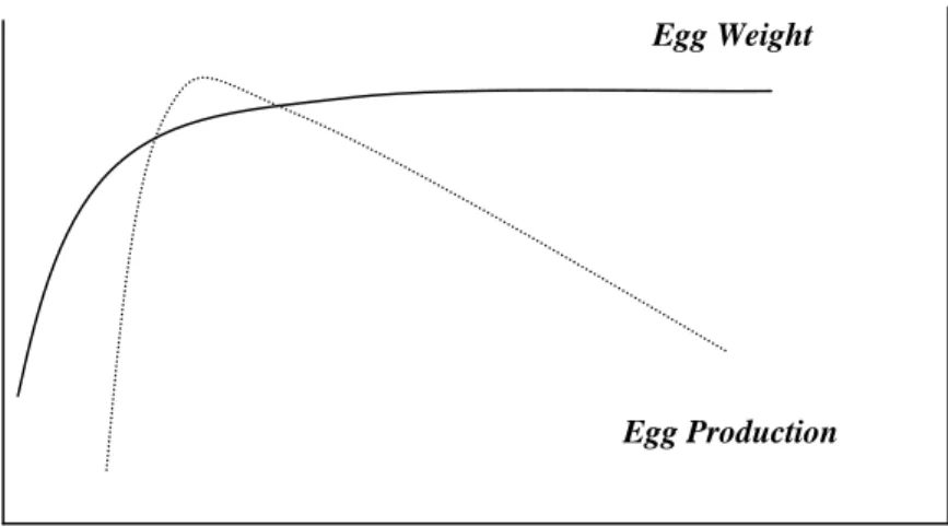
The age of laying hens is important because of the quality of hatching eggs is singularly determined by the age of the laying hens. According to Appleby, Hughes and Elson (1992), the production of eggs takes place from hens 20-72 weeks old and the best quality eggs come from hens age 28-32 weeks. During that period, egg production is at peak and the egg mass is optimal. Even though eggs from the older laying hens are normally bigger, egg shell thickness and strength decline, thus, increasing the proportion of cracked and broken eggs. In addition, the internal egg quality becomes poorer: the proportion of water in the albumen increases with age, resulting in unacceptably watery whites. Specifically, albumen quality is very important in determining the quality of chicks where the older flock will have a significantly lower albumen quality (Cunningham, Cotterill and Funk, 1960; Walsh, 1993). Figure 1 demonstrates those relationships graphically.

For the purposes of estimating (15) we use two measures of chick quality. First, we postulate that the best quality chicks come from eggs produced by laying hens that are at the most productive period of their lives which is at the age of about 30 weeks. To fit the empirical distribution of eggs/chicks quality from Figure 1 we use the Poisson distribution that has the property that it is uniquely specified by the mean (30 weeks). The distribution is skewed to the right and the density function drops gradually after it reaches the peak of the distribution. The quality variable (Q ) is then approximated by the height _i

of the Poisson distribution.

Second, we introduce a measurement of the flock genetic uniformity to capture the idea that less genetic variation among chicks in a given flock is performance enhancing. In this case, the quality variable is measured by the interaction between the age of the laying hen and the percentage of the flock coming from a single, most prevalent breed. We calculate this interaction by multiplying the height of the Poisson distribution with the percentage of the prevalent breed. Clearly, the highest possible quality chicks will come from the situation where 100% of eggs come from a single breed of laying hens of age 30 weeks.

The RHS variable in (15) is the grower’s ability. We assume that the ability of each grower can be accurately measured by his historical production performance relative to the group average performance where the production performance is measured by the per-pound settlement costs as previously defined. There are two reasons why this approach seems sensible. First, by comparing the individual settlement costs by the tournament average settlement costs the common production shock is filtered away and hence of no consequence to the individual performance. Second, by looking at the historical performance over multiple flocks, the importance of individual grower idiosyncratic shock should also gradually fade as its expected value is zero. Therefore the historical relative performance should accurately measure grower’s inherent characteristics, those that make him a better or a worse grower then the rest of the group.7

However, the presented approach suffers from the endogeneity problem reflected by the fact that the outcome of a tournament, and consequently the ranking of growers

with respect to their abilities, can be biased by the integrator via a strategic allocation of varying quality inputs across growers. In this case, what we believe to be an independent measure of grower’s ability could have in fact been obscured by the uneven allocation of inputs by the integrator. In other words, some growers ended up performing well not because they have superior abilities for growing chickens but because they were favored by the integrator who supplied them with high quality inputs. We will try to resolve this issue in the econometric model in the next section.

The historical performance variable for each grower (Hi) is calculated as the

average value of all relative performances up to the last tournament the grower participated in. For each grower this was done by first calculating the percentage difference between the grower’s settlement cost and the group average settlement cost for the first settlement date in the data set. This procedure is then repeated for every settlement date and the grower’s rank is updated by averaging his performances up to that point and comparing it with historical performance averages of other growers in the profit center. These series are constructed to simulate the integrator’s updating information about growers’ abilities after each round of tournaments has been played.

4.2 Econometric Model and Results

Given the fact that grower ability is not directly observable, the integrator need to develop a systematic method of formulating and updating their beliefs about growers’ relative abilities. Suppose that the integrator ranks an individual grower i in terms of his average relative settlement costs up to period t, labeled as H_i,t and that she updates her

information based on the following geometric lag distribution model ) ( ) 1 ( ] [ _{i i,t t 1 i} t A = − H + Ε− A Ε λ λ (16)

where ≤ λ<1. Expanding the last term gives

...) )( 1 ( ] [ 2 _{, 2} 1 , , + + + − = Εt Ai λ Hit λHit₋ λ Hit₋ . (17)

Substituting (17) into (15) and estimating (15) would involve infinite number of regressors, hence we apply Kyock transformation to obtain

7

The grower’s inherent characteristics in this context may be his abilities and skills but also other factors contributing to his productivity such as the quality and the vintage of the chicken houses (ventilation, insulation, etc.) as well as the location (grower being close to a processing plant or a feed mill).

1 , , 1 ,t+ = (1− )+ (1− ) it + it + t+ i H Q Q α λ γ λ λ κ . (18)

If estimated directly, (18) will produce inconsistent parameter estimates (see Kmenta, 1986, p.528-532). Therefore we use the instrumental variable (IV) approach and regress

t i

Q, on Hi,t−1 in the first step to obtain the predicted value of Qi,t and then estimate (18)

using Qˆ in the second step. _i,t

The evidence of the non-commitment behavior of the integrator is revealed through γ >0 (or γ <0) and λ∈[0,1) where the former reflects the discrimination based on abilities and the latter reflects integrator’s learning. When λ =1, there is no learning and thus no discrimination among growers. We estimate two models using two different measurements of the input quality variable discussed earlier. The results are reported in Table 2. The Durbin’s h-test8 is also performed to test for the presence of correlation between the predicted value from the first stage and the error term.

The results indicate that there is no significant relationship between the growers’ historical performance and the quality of inputs they currently receive. In three out of five contracts the estimated γ −(1 λ) are positive but all of them are not significantly different from zero. Based on the F-tests, we could not reject the hypothesis of that γ(1−λ)=0 and λ=1. The quality of chicks given to growers appears to be following random walk where the best prediction for the quality of chicks received in this period is the quality of chicks received in the previous period. These results do not support our hypotheses about strategic behavior of integrators when it comes to discrimination of growers regarding the distribution of variable quality inputs.

5. Conclusions

This research has been motivated by the frequent complaints of contract broiler growers that they have been treated unfairly in the hands of the integrators. Specifically, we investigated a problem of post-contractual opportunism (lack of long term commitment) on the part of the principal that can manifest itself in the strategic allocation

of variable quality inputs among growers of different abilities. The problem stems from the fact that the integrator-grower relationship is long-term (as determined by the useful life of the contract specific fixed assets acquired by both sides), yet the relationship is governed by the repeated short-term contracts. Observing the performance of contract growers over time, the integrator can make reasonably precise conjectures about grower abilities. Having this information, there is a temptation to deviate from the original explicit contract provisions and discriminate among growers when it comes to supplying them with the production inputs of varying quality.

Without having completely reliable information about the technology, it is impossible to predict what kind of strategy would the integrators pursue and what kind of dynamic response from growers would this strategy create. Based on some survey results and ample anecdotal evidence we believe that the incentives clearly exist for the integrator to supply high ability growers with high quality inputs and low ability growers with low quality inputs. This strategy would generate a career concerns type of dynamic response from the growers, who would be eager to win in the current period tournament not only because of the direct incentives they face, but also because of the fact that winning in the current period would improve their chances of obtaining the high quality inputs in the subsequent tournaments.

Our analysis shows no empirical support for this type of strategic behavior, nor do we find any empirical evidence for the alternative technological specification that would create a ratchet effect. We conclude that the empirical evidence is conformable with the full commitment type of behavior on the part of the integrators.

The main caveat of this study comes from the fact that we ignore the presence of potentially significant transaction costs that may be associated with either one of the mentioned integrators strategy. The transaction costs in this context would include the tangible costs of segregating inputs into categories (high or low) and the costs of delivering different categories of inputs to different growers, but also “shadow” costs

8 Durbin’s h = λ Q6 Q G −

− where d = Durbin-Watson’s statistics, n = number of observations,

λ

6 = estimated variance of the least square estimator of λ. The null hypothesis is that K~N(0,1) thus, no

associated with the loss of goodwill and good reputation among growers. The size of the transaction costs associated with the implementation of discrimination strategy may eliminate all potential benefits that the discrimination strategy would generate, or similarly, the benefits associated with strategic distribution of variable quality inputs as captured by the improved cost efficiency (reduced feed conversion) may be rather small. The high transaction costs (or small benefits) may prevent the integrator from engaging in this type of strategic behavior and may force him to stick with the commitment to distribute inputs fairly as implicitly understood in the short-term contracts.

References

Allen, D.W. and D. Lueck (1999). “Searching for Ratchet Effects in Agricultural Contracts.” Journal of Agricultural and Resource Economics, 24: 536-552.

Appleby, M.C., B.O. Hughes and H.A. Elson (1992). Poultry Production Systems:

Behavior, Management and Welfare Wallingford, U.K., C.A.B. International.

Berliner, J.S. (1957). Factory Manager in the Soviet Union. Cambridge, Harvard University Press.

Cunningham, F.E., D.J. Cotterill., and E.M. Funk (1960). “The Effect of Season and Age of Bird on the Chemical Composition of Egg white.” Poul. Sci. 39: 300-308.

Freixas, X., R. Guesnerie and J. Tirole (1985). “Planning under Incomplete Information and the Ratchet Effect.” Review of Economic Studies, 52: 173-191.

Holmstrom, B. (1999). “Managerial Incentive Problems: A Dynamic Perspective.”

Review of Economic Studies, 66: 169-182.

Ilvento, T., and A.Watson (1998). “Poultry Growers Speak Out: A Survey of Delmarva Poultry Growers.” College of Agriculture and Natural Resources, University of Delaware.

Kmenta, J. (1986). Elements of Econometrics. Ann Arbor, MI, The University of Michigan Press.

Knoeber, C., and W. Thurman (1994). “Testing the Theory of Tournaments: An Empirical Analysis of Broiler Production,” Journal of Labor Economics 12: 155-179.

Laffont, J.-J. and J. Tirole (1993). A Theory of Incentives in Procurement and Regulation. Cambridge, Mass.: The MIT Press.

Levy, A. and T. Vukina (2002). “Optimal Linear Contracts with Heterogeneous Agents.”

European Review of Agricultural Economics, Vol. 29 (2): 1-13 (in press).

Lewin-Solomons, S. (2000). “Asset Specificity and Hold-up in Franchising and Grower Contracts: A Theoretical Rationale for Government Regulation?” Working

Paper, Iowa State University.00.

Macho-Stadler, I. and D. Perez-Castrillo (1997). An Introduction to the Economics of

Meyer, M.A. (1995) “Cooperation and Competition in Organizations: A Dynamic Perspective.” European Economic Review, 39: 709-722.

Meyer, M.A. and J. Vickers (1997). “Performance Comparisons and Dynamic Incentives.” Journal of Political Economy, 105 (3): 547-581.

Salanie, B. (1997). The Economics of Contracts: A Primer. Cambridge, Mass.: The MIT Press.

Tsoulouhas, T., and T. Vukina (1999). “Integrator Contracts With Many Agents and Bankruptcy.” American Journal of Agricultural Economics, 81: 61-74.

Tsoulouhas, T., and T. Vukina (2001). “Regulating Broiler Contracts: Tournaments versus Fixed Performance Standards.” American Journal of Agricultural

Economics, 83: 1062-1073.

Walsh T.J. (1993). “The Effect of Flock Age, Storage Temperature, Storage Humidity, Carbon Dioxide and Length of Storage on Albumen Characteristics, Weight Loss and Embryonic Development of Broiler Eggs.” Ph.D. Dissertation, North Carolina State University.

Vukina, T. (2001). “Vertical Integration and Contracting in the U.S. Poultry Sector.”

Journal of Food Distribution Research, Vol. 32: 29-38.

Weitzman, M.L. (1980). “The “Ratchet Principle” and Performance Incentives.” The Bell Journal of Economics, Vol. 11 (1): 302-308.

Yao, D. (1988). “Strategic Responses to Automobile Emissions Control: A Game-Theoretic Analysis.” Journal of Environmental Economics and Management, Vol. 15: 419-438.

Appendix

Proof of Proposition 2:

From the maximization problem in the non-commitment case, equation (9) and (10) can be written as     ₋ + = )( ) 2 ( 2 * * 2 * * 2 * * 1 i j i r e e r e δ β (19)         − − = )( ) 2 ( 2 * * 2 * * 2 * * 1 i j j j j r e e r e θ β δ θ (20)

[

( )

]

2 2 * * 1 * * 1 * * 2 i j i e e r r e = + β − (21)

[

( )

]

2 2 * * 1 * * 1 * * 2 i j j j j e e r r e = − β − θ θ (22)

From these first-order conditions, we obtain the closed form solutions **2 * * 1 * * 2 * * 1, i , j , j i e e e e as

shown in equation (11) to (14). We claim that when β >0, e_i*₁* >e_i*₁ and e*_j*₁ <e*_j1 as

well as *2 * * 2 i i e e > and *2 * * 2 j j e e < .

We first prove e_i*₁* >e_i*₁ by showing that the contradictory statement can never be true. From (11) it follows that

2 1 1 1 1 ) 1 1 ( 2 ) 1 1 ( 2 2 2 2 2 2 r M QJ M rM M r J j j j j j j j >         + −         − + + −         − + θ θ β θ θ β θ θ β θ (23) where 1 (1 1 ) j j M J θ θ β ₊ − = , 1 (1 1 ) j M Q θ β + − = , 0 4 2 > = δβr M , and θ_j >1, the RHS of (23) is the e . The LHS is _i*₁ e . Rearranging terms by multiplying both the numerator *_i1*

and the denominator of the LHS by θ_j, we get the inequality

        + − < − + + − − + 2 2 2 2 2 ) 1 1 ( 2 ) 1 1 ( ) 1 1 ( 2 ) 1 1 ( 2 j _{j j j} j _j j M QJ r M rM M J r J θ β θ θ β θ β θ θ θ

Substituting Jand Q , < − + + −         + − − (1 1 ) (1 1 ) 2 ) 1 1 ( 1 ) 1 1 ( 2 ₂ j j j j j j M rM M M θ β θ β θ θβ θ θ 2 2 2 ) 1 1 ( 2 1 ) 1 1 ( 1 ) 1 1 ( 1 2 _{j j j j} j r M M M r θ β θ β θ θ β θ + −         − + −         + −

and rearranging terms gives

< − + + − + + + − − (1 1 ) (1 1 ) 2 ) 1 1 ( ) 1 1 ( ) 1 ( 2 2 ₂ 2 j j j j j j M rM M M M θ β θ β θ β θ θ β θ 2 2 2 2 2 2 ) 1 1 ( 2 ) 1 1 ( 2 ) 1 1 ( 2 _{j j j j} jM rM r M r θ β θ θβ θ β θ + − + + + −

From the fact that 2(1+ 1 )=

j M θ β 2(1 1₂) j M θ β − (1 1 ) 2 j j M θ θ β ₊ + , we get ) 1 1 ( ) 1 1 ( 2 ) 1 1 ( 2 ) 1 1 ( 2 ) 1 ( 2 2 2 − + + + − < + − − j j j j j j rM M r rM M θ θ β θ β θ θ β θ Therefore,

[

]

(1 1 ) (1 1 ) 0 2 1 ) 1 1 ( 2 ) 1 ( 2 2 2 < − + + − + + − j j j j j rM rM M θ θ β θ θ β θ (24)

However, as θ_j >1 and r,M,β >0, (24) can never be true. Hence, it must be that (23) is always true and *1

* * 1 i i e e > . Next we prove *1 * * 1 j j e

e < . If the claim is correct then it must be true that,

j j j j j j r M QJ M rM M r Q θ θ β θ θ β θ β θ 2 1 1 1 1 ) 1 1 ( 2 ) 1 1 ( 2 2 2 2 2 2 <         + −         − − + −         − − (25)

where the LHS of (25) is the e (equation (12)) and RHS of (21) is the *_i1* e*_j1. By

contradiction we get         + − > − − + − − + 2 2 2 2 2 2 ) 1 1 ( 2 ) 1 1 ( ) 1 1 ( 2 ) 1 1 ( 2 _{j j j j} jJQ M _j r M rM QM Qr θ β θ θ θ β θ β θ

Substituting Jand Q , > − − + −         + − − (1 1 ) (1 1 ) 2 ) 1 1 ( 1 ) 1 1 ( 2 ₂ j j j j M rM M M θ β θ β θ β θ ) 1 1 ( 2 1 ) 1 1 ( 1 ) 1 1 ( 1 2 2 2 2 j j j j j M r M M r θ θ β θ θ β θ β − +         − + −         + −

and rearranging terms

> − − + − + − + + − (1 1 ) (1 1 ) 2 ) 1 1 ( ) 1 1 ( ) 1 1 ( 2 ₂ 2 2 j j j j j j M rM M M M θ β θ β θ θ β θ β θ ) 1 1 ( 2 ) 1 1 ( 2 ) 1 1 ( 2 2 2 2 2 2 2 j j j j j j M r rM rM θ θ β θ θβ θ θβ + + + − + −

From the fact that 2(1+ 1 )=

j M θ β 2(1 1₂) j M θ β − (1 1 ) 2 j j M θ θ β ₊ + , we get 0 1 1 ) 1 1 ( 2 ) 1 1 ( >         − + + − j j j rM M θ θ β θ (26)

The LHS of (26) is always negative because θ_j >1and r,M,β >0. Therefore, it must be that (25) is true and *1

* *

1 j j e

e < .

To prove e*_i2* >e_i*₂, use (11)-(12) that imply

                        + −         − + + − + − = − ₂ 2 2 2 2 * * 1 * * 1 1 1 1 1 2 ) )( 1 1 ( ) ( 2 j j j j j j j i M QJ M Q J M Q J r e e θ β θ θ β θ θ θ (27)

The expression is always positive because J >Q if θ_j >1. Further, using

2 *

2

r e_i = , we can rewrite equation (13) as follows

2 * 2 * * 2 β r e e_i = _i +                         + −         − + + − + − 2 2 2 2 2 1 1 1 1 2 ) )( 1 1 ( ) ( 2 j j j j j j M QJ M Q J M Q J r θ β θ θ β θ θ θ

The second term on the RHS is positive. So, it must be that e_i*₂* >e_i*₂. For proving e*_j*₂ <e*_j2, we use the fact that

j j r e θ 2 *

2 = and rewrite equation (14),

j j j r e e θβ 2 * 2 * * 2 = −                         + −         − + + − + − 2 2 2 2 2 1 1 1 1 2 ) )( 1 1 ( ) ( 2 j j j j j j M QJ M Q J M Q J r θ β θ θ β θ θ θ

The second term on the RHS is positive, so it must be that e*_j*₂ <e*_j2.

Q.E.D.

Proof of Proposition 3:

We already proved in (27) that e_i*₁* −e*_j*₁ is positive. It is easy to verify that * * 2 * * 2 j i e

e − has a higher value than (27). From (13)-(14), we obtain

                        + −         − + + − + − + + − = − ₂ 2 2 2 2 * * 2 * * 2 1 1 1 1 2 ) )( 1 1 ( ) ( 2 ) 1 1 ( 2 ) 1 1 ( 2 j j j j j j j j j i M QJ M Q J M Q J r r r e e θ β θ θ β θ θ θ θ β θ (28) We can see that the value in (28) is greater than (27) because θ_j >1, hence

* * 1 * * 1 * * 2 * * 2 j i j i e e e e − > − . Q.E.D.

Table 1: Summary statistics of the Data Set Contract Number Number of Tournaments Number of usable Observations

Average Number of Growers per Tournament RB 45 830 18 RFF1 104 1202 12 LB 104 3194 31 RSR 104 937 9 RFF2 76 810 13