Copyright © 2004 - 2016 Ion Vasilief Copyright © 2010 Stephen Besch
Copyright © 2006 - june 2007 Roger Gadiou and Knut Franke
Legal notice:Permission is granted to copy, distribute and/or modify this document under the terms of theGNU Free Documen-tation License, Version 1.1 or any later version published by the Free Software Foundation; with no Invariant Sections, with no Front-Cover Texts, and with no Back-Cover Texts.
COLLABORATORS TITLE:
The QtiPlot Handbook
ACTION NAME DATE SIGNATURE
WRITTEN BY Ion Vasilief and Stephen Besch
The 13th of August 2016
REVISION HISTORY
Contents
1 Introduction 1
1.1 What QtiPlot does. . . 1
1.2 Command Line Parameters . . . 1
1.2.1 Specify a File . . . 1
1.2.2 Command Line Options . . . 2
1.3 General Concepts and Terms . . . 2
1.3.1 Tables. . . 5
1.3.2 Excel workbooks . . . 6
1.3.3 Matrix. . . 8
1.3.4 Plot Window . . . 8
1.3.5 Note. . . 9
1.3.6 Results Log Window . . . 10
1.3.7 The Project Explorer . . . 11
1.4 Interoperability with other scientific software . . . 11
1.4.1 OriginLab. . . 11
1.4.1.1 Import of OriginLab projects . . . 11
1.4.1.2 Export QtiPlot projects to OriginLab . . . 11
1.4.2 Microsoft Excel. . . 15
1.4.2.1 Import of Excel files . . . 15
1.4.2.2 Export QtiPlot data to Excel. . . 15
1.4.3 LibreOffice and Apache OpenOffice . . . 15
1.4.3.1 Import . . . 15
1.4.3.2 Export . . . 15
2 Drawing plots with QtiPlot 16 2.1 2D plots . . . 16
2.1.1 2D plot from data. . . 16
2.1.2 2D plot from function. . . 19
2.1.2.1 Direct plot of a function. . . 19
2.2 3D plots . . . 21
2.2.1 Direct 3D plot from a function . . . 22
2.2.2 3D plot from a matrix . . . 24
2.3 Multilayer Plots . . . 25
2.3.1 Building a multilayer plot panel . . . 25
2.3.2 Building a multilayer plot step by step . . . 26
3 Command Reference 29 3.1 The File Menu. . . 29
3.1.1 File-> New ->. . . 29
3.1.1.1 New -> New Project(Ctrl-N). . . 29
3.1.1.2 New -> New Folder(F7) . . . 29
3.1.1.3 New -> New Table(Ctrl-T) . . . 29
3.1.1.4 New -> New Excel . . . 30
3.1.1.5 New -> New Matrix(Ctrl-M). . . 30
3.1.1.6 New -> New Note . . . 30
3.1.1.7 New -> New Graph(Ctrl-G) . . . 31
3.1.1.8 New -> New Function Plot -> New Function Plot...(Ctrl-F) . . . 31
3.1.1.9 New -> New Function Plot -> New Parametric Function Plot... . . 32
3.1.1.10 New -> New Function Plot -> New 3D Surface Plot...(Ctrl-Alt-Z) . . . 32
3.1.1.11 New -> New Function Plot -> New 3D Parametric Surface Plot... . . 32
3.1.2 File ->Open(Ctrl-O) . . . 32
3.1.3 File ->Open Excel . . . 32
3.1.4 File ->Open ODF Spreadsheet. . . 32
3.1.5 File->Open Image File(Ctrl-I) . . . 32
3.1.6 File ->Append Project...(Ctrl-Alt-A) . . . 32
3.1.7 File->Recent Projects. . . 32
3.1.8 File ->Close . . . 33
3.1.9 File->Save Project(Ctrl-S) . . . 33
3.1.10 File->Save Project as...(Ctrl-Shift-S) . . . 33
3.1.11 File->Save Window as... . . 33
3.1.12 File ->Open Template . . . 33
3.1.13 File ->Save as Template . . . 34
3.1.14 File->Print(Ctrl-P) . . . 34
3.1.15 File->Print Preview . . . 34
3.1.16 File->Print All Plots . . . 34
3.1.17 File ->Export Graph . . . 34
3.1.17.1 Export Graph -> Current(Alt-G) . . . 34
3.1.17.3 File -> Create Open Document Presentation... . . 35 3.1.18 File ->Export . . . 35 3.1.18.1 Export ASCII . . . 35 3.1.18.2 Export Excel . . . 35 3.1.18.3 Export to PDF(Ctrl-Alt-P) . . . 35 3.1.19 File -> Import. . . 35
3.1.19.1 File ->Import -> Import ASCII...(Ctrl-K) . . . 35
3.1.19.2 File->Import Image... . . 35
3.1.19.3 File ->Import -> Database... . . 36
3.1.19.4 File ->Import -> Matlab... . . 36
3.1.19.5 File ->Import -> Sound (WAV)... . . 36
3.1.19.6 File ->Import -> NI (TDMS)... . . 36
3.1.20 File ->Quit(Ctrl-Q) . . . 36
3.2 The Edit Menu . . . 36
3.2.1 Edit ->Undo(Ctrl-Z) . . . 36
3.2.2 Edit ->Redo(Ctrl-Shift-Z). . . 37
3.2.3 Edit ->Cut Selection(Ctrl-X) . . . 37
3.2.4 Edit ->Copy Selection(Ctrl-C) . . . 37
3.2.5 Edit ->Paste Selection(Ctrl-V) . . . 37
3.2.6 Edit ->Delete Selection(Del) . . . 37
3.2.7 Edit ->Delete Fit Tables. . . 37
3.2.8 Edit ->Clear Log Information . . . 37
3.2.9 Edit ->Preferences... . . 37
3.3 The View Menu . . . 37
3.3.1 View ->Toolbars...(Ctrl-Shift-T) . . . 37
3.3.2 View ->Project Explorer(Ctrl-E) . . . 37
3.3.3 View ->Results log . . . 38
3.3.4 View ->Undo/Redo Stack.... . . 38
3.3.5 View ->Show/Hide Scripting Console . . . 38
3.4 The Scripting Menu . . . 38
3.4.1 General Scripting Commands . . . 38
3.4.1.1 Scripting ->Scripting language . . . 38
3.4.1.2 Scripting ->Restart scripting . . . 38
3.4.1.3 Scripting ->Add Custom Script Action... . . 38
3.4.2 Notes Specific Scripting Commands . . . 38
3.4.2.1 Scripting ->Execute(Ctrl+J) . . . 38
3.4.2.2 Scripting ->Preferences...(Ctrl+Shift+J) . . . 38
3.4.2.3 Scripting ->Evaluate(Ctrl+Return) . . . 39
3.4.2.5 Add Tab . . . 39
3.4.2.6 Close Tab . . . 39
3.5 The Graph Menu . . . 39
3.5.1 Graph ->Add/Remove Curves...(Alt-C) . . . 39
3.5.2 Graph ->Add Function...(Ctrl-Alt-F) . . . 39
3.5.3 Graph ->Add Error Bars...(Ctrl-B) . . . 39
3.5.4 Graph ->Rescale To Show All(Ctrl-Shift-R) . . . 39
3.5.5 Graph ->Exchange X-Y Axes . . . 39
3.5.6 Graph ->New Legend(Ctrl-L) . . . 40
3.5.7 Graph ->Add Equation...(Alt-Q). . . 40
3.5.8 Graph ->Add Text(Alt-T). . . 40
3.5.9 Graph ->Draw Arrow(Ctrl-Alt-A) . . . 40
3.5.10 Graph ->Draw Line(Ctrl-Alt-L) . . . 40
3.5.11 Graph ->Add Rectangle(Ctrl-Alt-R) . . . 40
3.5.12 Graph ->Add Ellipse(Ctrl-Alt-E) . . . 40
3.5.13 Graph ->Add Time Stamp(Ctrl-Alt-T). . . 40
3.5.14 Graph ->Add Image(Alt-I) . . . 41
3.5.15 Graph -> Add Central Axis. . . 41
3.5.15.1 Add Horizontal Axis . . . 41
3.5.15.2 Add Vertical Axis. . . 41
3.5.16 Z-Order Commands... . . 41
3.5.16.1 Move to Top. . . 41
3.5.16.2 Move to Bottom. . . 41
3.5.17 Graph ->Add Layer(Alt-L). . . 41
3.5.18 Graph ->Add Empty Inset Layer . . . 42
3.5.19 Graph ->Add Inset Layer With Curves . . . 42
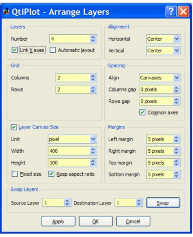
3.5.20 Graph ->Arrange Layers(Shift-A) . . . 42
3.5.21 Graph ->Automatic Layoutcommand . . . 42
3.5.22 Graph ->Extract to Graphscommand . . . 42
3.5.23 Graph ->Extract to Layerscommand . . . 42
3.5.24 Graph ->Remove Layer(Alt-R) . . . 42
3.6 The Plot Menu . . . 42
3.6.1 Plot Wizard(Ctrl-Alt-W) . . . 43
3.6.2 Line -> . . . 43 3.6.2.1 Line . . . 43 3.6.2.2 Line Central . . . 43 3.6.2.3 Vertical Steps . . . 43 3.6.2.4 Horizontal Steps . . . 44 3.6.3 Symbol -> . . . 44
3.6.3.1 Scatter. . . 44
3.6.3.2 Scatter Central . . . 45
3.6.3.3 Vertical Drop Lines. . . 45
3.6.4 Line + Symbol -> . . . 46
3.6.4.1 Line+Symbol . . . 46
3.6.4.2 Line + Symbol Central . . . 46
3.6.4.3 Spline . . . 46 3.6.5 Column/Bar/Pie -> . . . 47 3.6.5.1 Columns. . . 47 3.6.5.2 Rows. . . 47 3.6.5.3 Stack Column. . . 48 3.6.5.4 Stack Bar . . . 48 3.6.5.5 100% Stack Column . . . 49 3.6.5.6 100% Stack Bar . . . 49 3.6.5.7 Floating Column . . . 49 3.6.5.8 Floating Bar . . . 50
3.6.5.9 3D Color Pie Chart. . . 50
3.6.5.10 2D BW Pie Chart . . . 50
3.6.6 Multi-Curve -> . . . 50
3.6.6.1 Double-Y . . . 50
3.6.6.2 Stack Lines by Y Offsets . . . 51
3.6.6.3 Waterfall . . . 51 3.6.7 Area -> . . . 51 3.6.7.1 Area . . . 51 3.6.7.2 Stack Area . . . 52 3.6.7.3 100% Stack Area . . . 52 3.6.7.4 Fill Area. . . 52 3.6.8 Special Line/Symbol -> . . . 52 3.6.8.1 Vectors XYXY . . . 52 3.6.8.2 Vectors XYAM . . . 53 3.6.8.3 Zoom . . . 53 3.6.9 Statistical Graphs -> . . . 54 3.6.9.1 Box Plot . . . 54 3.6.9.2 Histogram. . . 54 3.6.9.3 Histogram + Probabilities . . . 55 3.6.9.4 Stacked Histogram . . . 55
3.6.9.5 Stem and Leaf . . . 55
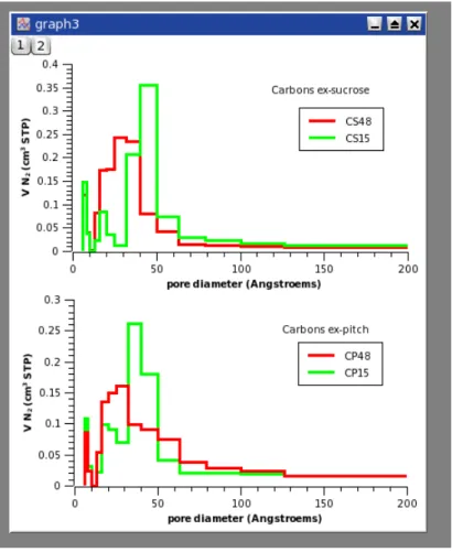
3.6.10 Panel -> . . . 56
3.6.10.2 Horizontal 2 Layers . . . 56 3.6.10.3 4 Layers . . . 56 3.6.10.4 Stacked Layers . . . 56 3.6.10.5 Custom Layout... . . 56 3.6.11 Data -> Plot 3D -> . . . 56 3.6.11.1 Ribbons . . . 56 3.6.11.2 Bars . . . 57 3.6.11.3 Scatter. . . 57 3.6.11.4 Trajectory. . . 57
3.7 The 3D Plot menu. . . 58
3.7.1 3D Wire Frame . . . 58 3.7.2 3D Hidden Lines. . . 58 3.7.3 3D Polygons . . . 59 3.7.4 3D Wire Surface. . . 59 3.7.5 Bars . . . 60 3.7.6 Scatter . . . 60 3.7.7 Contour+Color Fill . . . 60 3.7.8 Countour Lines . . . 61
3.7.9 Gray Scale Map . . . 61
3.8 The Data Menu . . . 61
3.8.1 Data ->Disable tools. . . 62
3.8.2 Data ->Zoom In/Out and Drag Canvas . . . 62
3.8.3 Data ->Zoom/Drag Canvas Horizontally . . . 62
3.8.4 Data ->Zoom/Drag Canvas Vertically . . . 62
3.8.5 Data ->Zoom in(Ctrl-+). . . 63
3.8.6 Data ->Zoom out(Ctrl--) . . . 63
3.8.7 Data ->Select Data Range(Alt-S) . . . 63
3.8.8 Data ->Data Reader(Ctrl-D) . . . 63
3.8.9 Data ->Annotation . . . 63
3.8.10 Data ->Screen Reader . . . 63
3.8.11 Data ->Draw Data Points . . . 64
3.8.12 Data ->Move Data points(Ctrl-Alt-M). . . 64
3.8.13 Data ->Remove Bad Data Points(Alt-B) . . . 64
3.8.14 Data ->Remove Bad Data Points . . . 64
3.9 The Analysis Menu . . . 64
3.9.1 Commands for the analysis of data in tables . . . 65
3.9.1.1 Descriptive Statistics . . . 65
3.9.1.1.1 Statistics on Columns . . . 65
3.9.1.1.3 Frequency Count. . . 65
3.9.1.1.4 Normality Test . . . 65
3.9.1.2 Hypothesis-Testing . . . 65
3.9.1.2.1 One Sample t-Test . . . 65
3.9.1.2.2 Two Sample t-Test . . . 66
3.9.1.3 ANOVA . . . 66 3.9.1.3.1 One-Way ANOVA . . . 66 3.9.1.3.2 Two-Way ANOVA . . . 66 3.9.1.4 Sort Column . . . 66 3.9.1.5 Sort Table . . . 66 3.9.1.6 Normalize . . . 66 3.9.1.6.1 Normalize -> Columns. . . 67 3.9.1.6.2 Normalize -> Table. . . 67 3.9.1.7 Differentiate Column . . . 67 3.9.1.8 Integrate Column . . . 67 3.9.1.9 FFT... . . 67 3.9.1.10 Correlate . . . 67 3.9.1.11 Autocorrelate . . . 67 3.9.1.12 Convolute . . . 67 3.9.1.13 Deconvolute . . . 67
3.9.1.14 Fit Wizard...(Ctrl-Y). . . 68
3.9.2 Commands for the analysis of curves in plots . . . 68
3.9.2.1 Translate . . . 68
3.9.2.1.1 Vertical . . . 68
3.9.2.1.2 Horizontal . . . 68
3.9.2.2 Subtract . . . 68
3.9.2.2.1 Subtract -> Baseline . . . 68
3.9.2.2.2 Subtract -> Reference Data . . . 69
3.9.2.2.3 Subtract -> Straight Line . . . 69
3.9.2.3 Peaks... . . 69 3.9.2.4 Differentiate . . . 69 3.9.2.5 Integrate Curve. . . 69 3.9.2.6 Integrate Function... . . 70 3.9.2.7 Smooth . . . 70 3.9.2.7.1 Savitski-Golay.... . . 70
3.9.2.7.2 Moving Window Average... . . 70
3.9.2.7.3 Lowess... . . 71
3.9.2.7.4 FFT Filter... . . 71
3.9.2.8.1 Low Pass... . . 72 3.9.2.8.2 High Pass... . . 72 3.9.2.8.3 Band Pass... . . 72 3.9.2.8.4 Band Block... . . 73 3.9.2.9 Interpolate... . . 73 3.9.2.10 FFT... . . 74 3.9.2.11 Fit Linear . . . 74 3.9.2.12 Fit Polynomial... . . 74
3.9.2.13 Fit Exponential Decay. . . 74
3.9.2.13.1 First Order... . . 74
3.9.2.13.2 Second Order... . . 74
3.9.2.13.3 Third Order... . . 74
3.9.2.14 Fit Exponential Growth... . . 75
3.9.2.15 Fit Boltzmann (sigmoidal) . . . 75
3.9.2.16 Fit Pseudo-Voigt . . . 75 3.9.2.16.1 PsdVoigt1... . . 75 3.9.2.16.2 PsdVoigt2... . . 75 3.9.2.17 Fit Gaussian . . . 75 3.9.2.18 Fit Lorentzian . . . 75 3.9.2.19 Fit Multi-peak . . . 75 3.9.2.19.1 Gaussian.... . . 75 3.9.2.19.2 Lorentzian... . . 75 3.9.2.19.3 PsdVoigt1... . . 75 3.9.2.19.4 PsdVoigt2... . . 75
3.9.3 Commands for the analysis of data in matrices . . . 76
3.9.3.1 Integrate . . . 76 3.9.3.2 FFT... . . 76 3.9.3.3 Forward FFT . . . 76 3.9.3.4 Inverse FFT. . . 76 3.9.3.5 FFT Filter. . . 76 3.9.3.5.1 Low Pass... . . 76 3.9.3.5.2 High Pass... . . 76 3.9.3.5.3 Band Pass... . . 76 3.9.3.5.4 Band Block... . . 77
3.10 The Table Menu . . . 77
3.10.1 Set Column As . . . 77
3.10.1.1 Set Column As -> X . . . 77
3.10.1.2 Set Column As -> Y . . . 77
3.10.1.4 Set Column As -> X error . . . 77
3.10.1.5 Set Column As -> Y error . . . 77
3.10.1.6 Set Column As -> Read-only . . . 77
3.10.1.7 Set Column As -> Read/Write. . . 77
3.10.1.8 Set Column As -> label. . . 77
3.10.1.9 Set Column As -> Disregard. . . 78
3.10.2 Column Options... . . 78
3.10.3 Set Column Values... . . 78
3.10.4 Recalculate. . . 78
3.10.5 Fill column with . . . 78
3.10.5.1 Fill Column With -> Row Numbers. . . 78
3.10.5.2 Fill Column With -> Random Numbers . . . 78
3.10.5.3 Fill Column With -> Normal Random Numbers. . . 78
3.10.6 Clear . . . 78
3.10.7 Add Column . . . 78
3.10.8 Set Columns... . . 79
3.10.9 Hide Selected Columns . . . 79
3.10.10Show All Columns. . . 79
3.10.11Set Optimal Column Width . . . 79
3.10.12Move to First . . . 79 3.10.13Move Left . . . 79 3.10.14Move Right . . . 79 3.10.15Move to Last. . . 79 3.10.16Swap columns . . . 79 3.10.17Set Rows... . . 79
3.10.18Delete Rows Interval... . . 79
3.10.19 Move Row . . . 80
3.10.19.1Move Row -> UP . . . 80
3.10.19.2Move Row -> DOWN. . . 80
3.10.20Go to Row...(Ctrl-Alt-G) . . . 80
3.10.21Go to Column...(Ctrl-Alt-C) . . . 80
3.10.22Extract Data... . . 80
3.10.23Convert to Matrix . . . 80
3.11 The Matrix Menu . . . 80
3.11.1 Set Properties... . . 80
3.11.2 Set Dimensions...(Ctrl-D) . . . 80
3.11.3 Set Values...(Ctrl-Q). . . 81
3.11.4 Recalculate(Ctrl-Return) . . . 81
3.11.6 Rotate -90(Ctrl-Alt-R). . . 81 3.11.7 Flip V(Ctrl-Shift-V) . . . 81 3.11.8 Flip H(Ctrl-Shift-H) . . . 81 3.11.9 Expand... . . 81 3.11.10Shrink... . . 81 3.11.11Smooth . . . 81 3.11.12Transpose . . . 81 3.11.13Invert. . . 81 3.11.14Determinant . . . 82 3.11.15 Go To Commands . . . 82 3.11.16 View Commands . . . 82
3.11.16.1Image mode(Ctrl-Shift-I) . . . 82
3.11.16.2Data mode(Ctrl-Shift-D) . . . 82
3.11.17 Palette. . . 82
3.11.17.1Gray Scale Map . . . 82
3.11.17.2Rainbow. . . 82
3.11.17.3Custom . . . 82
3.11.18Show Column/Row(Ctrl-Shift-C). . . 82
3.11.19Show X/Y(Ctrl-Shift-X) . . . 82
3.11.20Convert to Spreadsheet . . . 82
3.12 The Format Menu . . . 82
3.12.1 Plot... . . 83 3.12.2 Curves... . . 83 3.12.3 Scales... . . 83 3.12.4 Axes... . . 83 3.12.5 Grid... . . 83 3.12.6 Title.... . . 83
3.13 The Windows Menu. . . 83
3.13.1 Folders . . . 83 3.13.2 Cascade . . . 84 3.13.3 Tile . . . 84 3.13.4 Next (F5) . . . 84 3.13.5 Previous (F6) . . . 84 3.13.6 Find... . . 84 3.13.7 Rename Window . . . 84 3.13.8 Duplicate . . . 84 3.13.9 Script Window (F3). . . 84 3.13.10 Window Geometry... . . 84 3.13.11 Hide Window . . . 84
3.13.12 Close Window (Ctrl-W) . . . 84
3.13.13 Numbered Window List . . . 85
3.14 Customization of 3D plots . . . 85 3.14.1 Frame . . . 85 3.14.2 Box . . . 85 3.14.3 No axes . . . 85 3.14.4 Front Grid . . . 85 3.14.5 Back Grid . . . 85 3.14.6 Left Grid . . . 85 3.14.7 Right Grid . . . 85 3.14.8 Ceiling Grid . . . 86 3.14.9 Floor Grid . . . 86 3.14.10Enable perspective . . . 86 3.14.11Reset rotation . . . 86
3.14.12Fit frame to window. . . 86
3.14.13Bars Style . . . 86 3.14.14Dots. . . 86 3.14.15Cones. . . 86 3.14.16Cross Hairs . . . 86 3.14.173D Wire Frame . . . 87 3.14.183D Hidden Lines. . . 87 3.14.193D Polygons . . . 87 3.14.203D Wire Surface. . . 87
3.14.21Floor Data Projection . . . 87
3.14.22Floor Isolines . . . 87
3.14.23Empty Floor . . . 87
3.14.24Animation . . . 87
4 The Toolbars 88 4.1 The Edit Toolbar . . . 88
4.2 The File Toolbar. . . 88
4.3 The Plot Toolbar . . . 90
4.4 The Layers Toolbar . . . 90
4.5 The Table Toolbar. . . 90
4.6 The Column Toolbar . . . 93
5 The Dialogs 97
5.1 Add Custom Action . . . 97
5.2 Add Error bars . . . 97
5.3 Add Function . . . 99 5.4 Add Layer . . . 102 5.5 Add/Remove Curves . . . 102 5.6 Arrange Layers . . . 103 5.7 Line Options . . . 105 5.7.1 Line Tab . . . 105
5.7.2 Arrow Head Tab . . . 106
5.7.3 Geometry Tab. . . 106
5.7.4 Axes Tab . . . 107
5.8 Column Options. . . 107
5.9 Contour Curves Options . . . 108
5.10 Plot Details . . . 113 5.10.1 Dimensions . . . 113 5.10.2 Print. . . 114 5.10.3 Fonts . . . 114 5.10.4 Miscellaneous . . . 115 5.10.5 Window Display . . . 115 5.10.6 Legends/Titles . . . 116 5.10.7 Layer . . . 117 5.10.8 Canvas . . . 117 5.10.9 Geometry . . . 118 5.10.10 Speed . . . 119 5.10.11 Layer Display. . . 120 5.10.12 Stack . . . 120 5.10.13 Group Edit . . . 121
5.10.14 Custom curves for lines and scatter plots . . . 122
5.10.15 Custom error bars. . . 125
5.10.16 Plot Details for pie plots . . . 125
5.10.17 Custom curves for box plots . . . 127
5.10.18 Custom histograms . . . 129
5.10.18.1 Histogram Data Formatting . . . 130
5.11 Define surface plot . . . 130
5.12 Export Graph Dialog . . . 132
5.13 Export ASCII Dialog . . . 134
5.14 Fast Fourier Transform Dialog . . . 135
5.16 Find Peaks Dialog. . . 138
5.17 Baseline Dialog . . . 139
5.18 Integrate Function Dialog . . . 140
5.19 The Fit Wizard . . . 141
5.19.1 Select Function Tab. . . 141
5.19.2 Fitting Session Tab . . . 142
5.19.3 Custom Output Tab . . . 144
5.19.3.1 Reported errors . . . 144
5.19.3.2 Goodness-of-Fit Statistics . . . 144
5.20 General Plot Options . . . 145
5.20.1 Scale Tab . . . 145
5.20.2 Grid Tab . . . 146
5.20.3 Axis Tab . . . 147
5.20.4 Special Ticks Tab . . . 148
5.20.5 General Tab. . . 149
5.21 Plot Wizard . . . 150
5.22 Project Explorer Find Dialog . . . 151
5.23 Preferences Dialog . . . 152
5.23.1 General Preferences . . . 152
5.23.1.1 Application Tab . . . 153
5.23.1.2 Confirmations Tab . . . 154
5.23.1.3 Colors Tab . . . 155
5.23.1.4 Numeric Format Tab. . . 156
5.23.1.5 File Locations Tab . . . 157
5.23.1.6 Keyboard Tab . . . 158
5.23.1.7 Internet Connections Tab . . . 159
5.23.2 Tables Preferences . . . 160
5.23.3 2D Plot Preferences. . . 161
5.23.3.1 Options Tab . . . 161
5.23.3.2 Curves Tab. . . 162
5.23.3.3 Error Bars Tab . . . 163
5.23.3.4 Axes Tab. . . 164 5.23.3.5 Ticks Tab . . . 165 5.23.3.6 Grid Tab . . . 166 5.23.3.7 Geometry Tab . . . 167 5.23.3.8 Speed Tab . . . 168 5.23.3.9 Fonts Tab . . . 169 5.23.3.10 Print Tab . . . 170 5.23.4 3D Plot Preferences. . . 171
5.23.5 Notes Preferences. . . 172
5.23.6 Fitting Preferences . . . 173
5.24 Printer-setup. . . 174
5.25 Set Column Values . . . 175
5.26 Extract Data . . . 176
5.27 Set Matrix Dimensions . . . 177
5.28 Import ASCII files . . . 178
5.29 Matrix Properties . . . 180
5.30 Set Matrix Values . . . 180
5.31 Surface plot options . . . 181
5.31.1 Scale Tab . . . 181 5.31.2 Axis Tab . . . 181 5.31.3 Grid Tab . . . 182 5.31.4 Title Tab . . . 182 5.31.5 Data Tab . . . 183 5.31.6 Colors Tab . . . 183 5.31.7 3D Vectors Tab . . . 184 5.31.8 Legend Tab . . . 184 5.31.9 General Tab. . . 185 5.31.10 Print Tab . . . 186 5.32 Sorting Options . . . 187
5.33 Tex Equation Editor . . . 187
5.34 Text options . . . 189
6 Analysis of data and curves 193 6.1 Fast Fourier Transform . . . 193
6.2 Correlation . . . 194
6.3 Convolution . . . 195
6.4 Deconvolution. . . 195
6.5 The Fit Wizard . . . 195
6.6 Fitting to specific curves . . . 196
6.6.1 Fitting to a line . . . 196
6.6.2 Fitting to a polynomial . . . 197
6.6.3 Fitting to a Boltzmann function . . . 198
6.6.4 Fitting to a Gauss function . . . 199
6.6.5 Fitting to a Lorentz function . . . 200
6.6.6 Fitting to a PsdVoigt1 function . . . 201
6.6.7 Fitting to a PsdVoigt2 function . . . 201
6.8 Filtering of data curves . . . 202
6.8.1 FFT low pass filter . . . 203
6.8.2 FFT high pass filter . . . 204
6.8.3 FFT band pass filter . . . 205
6.8.4 FFT block band filter . . . 206
6.9 Interpolation. . . 207
7 Mathematical Expressions and Scripting 209 7.1 muParser . . . 209
7.2 Python . . . 209
7.2.1 The Initialization File. . . 209
7.2.2 Python Basics. . . 210
7.2.3 Defining Functions and Control Flow . . . 212
7.2.4 Mathematical Functions . . . 213
7.2.5 Accessing QtiPlot’s objects from Python . . . 213
7.2.6 Project Folders . . . 216
7.2.7 Working with Tables . . . 218
7.2.7.1 Import ASCII files . . . 222
7.2.7.2 Importing Excel sheets . . . 222
7.2.7.3 Importing ODF spreadsheets . . . 223
7.2.7.4 Export Tables . . . 223
7.2.7.5 R interface . . . 224
7.2.8 Working with Matrices . . . 224
7.2.9 Table/Matrix conversion . . . 227
7.2.10 Stem Plots . . . 228
7.2.11 2D Plots. . . 228
7.2.11.1 The plot title . . . 228
7.2.11.2 Customizing the axes . . . 229
7.2.11.3 The canvas . . . 232
7.2.11.4 The layer frame . . . 232
7.2.11.5 Customizing the grid . . . 233
7.2.11.6 The plot legend . . . 233
7.2.11.7 Antialiasing . . . 234
7.2.11.8 Resizing layers. . . 234
7.2.11.9 Resizing the drawing area . . . 235
7.2.11.10 Working with 2D curves. . . 235
7.2.11.11 Curve symbols . . . 240
7.2.11.12 Curve labels . . . 241
7.2.11.14 Selecting a data range . . . 243
7.2.11.15 2D Analytical Functions. . . 243
7.2.11.16 Error Bars . . . 244
7.2.11.17 Image and Contour Line Plots (Spectrograms) . . . 244
7.2.11.18 Histograms. . . 246
7.2.11.19 Box and whiskers plots . . . 246
7.2.11.20 Distribution Curves . . . 247
7.2.11.21 Pie Plots . . . 248
7.2.11.22 Vector Plots . . . 248
7.2.11.23 Adding arrows/lines to a plot layer . . . 248
7.2.11.24 Adding images to a layer . . . 250
7.2.11.25 Rectangles . . . 250 7.2.11.26 Circles/Ellipses . . . 250 7.2.11.27 Exporting graphs . . . 251 7.2.11.28 Arranging Layers . . . 252 7.2.11.29 Waterfall Plots . . . 253 7.2.12 3D Plots. . . 253 7.2.12.1 Creating a 3D plot . . . 253
7.2.12.2 Customizing the view . . . 254
7.2.12.3 Plot Styles . . . 255
7.2.12.4 3D Vectors . . . 256
7.2.12.5 The 2D Projection . . . 256
7.2.12.6 The Coordinates System. . . 257
7.2.12.7 Grid . . . 257
7.2.12.8 Customizing the Plot Colors. . . 258
7.2.12.9 Exporting . . . 258 7.2.13 Data Analysis. . . 259 7.2.13.1 General Functions . . . 259 7.2.13.2 Correlation, Convolution/Deconvolution . . . 260 7.2.13.3 Differentiation . . . 260 7.2.13.4 FFT . . . 261 7.2.13.5 FFT Filters. . . 261 7.2.13.6 Fitting . . . 262 7.2.13.7 Integration . . . 264 7.2.13.8 Interpolation . . . 265 7.2.13.9 Smoothing . . . 265 7.2.14 Statistics . . . 266 7.2.14.1 Descriptive Statistics . . . 266
7.2.14.3 One Sample Test for Variance (Chi-Square Test) . . . 267
7.2.14.4 Normality Test (Shapiro - Wilk). . . 267
7.2.14.5 One-Way ANOVA . . . 267
7.2.14.6 Two-Way ANOVA. . . 267
7.2.15 Working with Notes . . . 268
7.2.16 Using PyQt’s dialogs and classes. . . 269
7.2.17 Using Qt Designer for easy creation of custom user dialogs. . . 269
7.2.18 Task automation example. . . 269
7.2.19 Scope Changes . . . 272
7.2.20 QtiPlot/Python API . . . 272
7.2.21 PyQt Class Reference . . . 272
8 Frequently asked questions 273
List of Figures
1.1 A typical QtiPlot session . . . 3
1.2 The QtiPlot table . . . 5
1.3 Working with Excel workbooks in QtiPlot . . . 6
1.4 Context menu for Excel workbooks . . . 7
1.5 Properties dialog for Excel workbooks . . . 7
1.6 The QtiPlot matrix . . . 8
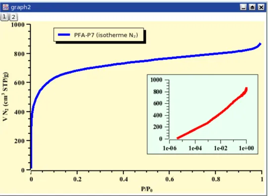
1.7 An example of QtiPlot 2D graph . . . 9
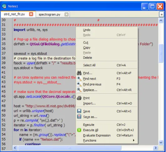
1.8 The QtiPlot Note Window . . . 10
1.9 The QtiPlot Results Log window . . . 10
1.10 The QtiPlot Project Explorer . . . 11
1.11 Export QtiPlot windows/projects as Origin C files . . . 12
1.12 OriginLab - Create new custom menu . . . 12
1.13 OriginLab - New custom menu . . . 13
1.14 OriginLab - New custom menu item . . . 13
1.15 OriginLab - Import script . . . 14
1.16 OriginLab - Select C file generated by QtiPlot . . . 15
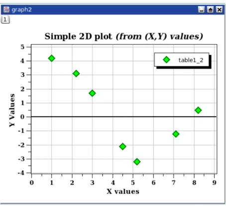
2.1 A simple 2D plot: the table.. . . 17
2.2 A simple 2D plot: the default plot. . . 17
2.3 A simple 2D plot: the plot finished. . . 18
2.4 A 2D plot with two Y axes. . . 18
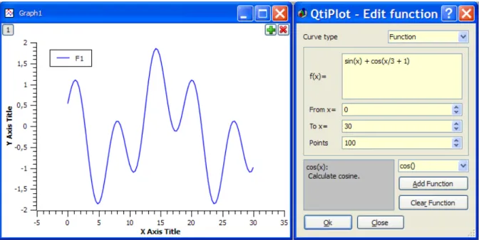
2.5 Direct plot of a function. . . 20
2.6 Function plot: filling of the X column. . . 20
2.7 Function plot: filling of the Y column. . . 21
2.8 Example of a 3D Plots. . . 22
2.9 Definition of a new surface 3D plot. . . 23
2.10 The 3D surface plot created using defaults . . . 23
2.11 The 3D surface plot after customization. . . 24
3.1 TheSmooth -> Savitsky-Golay...dialog. . . 70
3.3 TheSmooth -> Lowess...dialog.. . . 71 3.4 TheSmooth -> FFT Filter...dialog. . . 71 3.5 TheFFT Filter -> Low Pass...dialog. . . 72 3.6 TheFFT Filter -> High Pass...dialog. . . 72 3.7 TheFFT Filter -> Band Pass...dialog. . . 73 3.8 TheFFT Filter -> Band Block...dialog. . . 73 3.9 TheInterpolate...dialog.. . . 74 4.1 The QtiPlot Edit Toolbar . . . 88 4.2 The QtiPlot File Toolbar . . . 88 4.3 The QtiPlot Plot Toolbar . . . 90 4.4 The QtiPlot Layers Toolbar . . . 90 4.5 The QtiPlot Table Toolbar . . . 93 4.6 The QtiPlot Column Toolbar . . . 93 4.7 The QtiPlot Plot 3D Toolbar . . . 95 5.1 TheAdd Custom Script Action...dialog box. . . 97 5.2 TheAdd Error Bars...dialog. . . 98 5.3 Example of a plot with both X and Y Error Bars. . . 99 5.4 TheAdd Function...dialog box: Cartesian Coordinates. . . 100 5.5 TheAdd Function...Dialog Box: Automatic Detection of Constants. . . 100 5.6 TheAdd Function...dialog box: Parametric Coordinates. . . 101 5.7 TheAdd Function...dialog box: Polar Coordinates. . . 102 5.8 TheAdd LayerDialog Box. . . 102 5.9 TheAdd/Remove Curves...Dialog Box. . . 103 5.10 TheArrange Layersdialog: the Geometry Tab . . . 104 5.11 Example of a vertical arrangement for two plots.. . . 105 5.12 TheArrow OptionsDialog: Line Tab. . . 106 5.13 TheArrow OptionsDialog: Arrow Head Tab . . . 106 5.14 TheArrow OptionsDialog: Geometry Tab . . . 107 5.15 TheArrow OptionsDialog: Axes Tab . . . 107 5.16 TheColumn Options...Dialog. . . 108 5.17 The Values tab. . . 109 5.18 The Colors Tab. . . 110 5.19 The Contour Lines tab. . . 112 5.20 The Labels tab. . . 113 5.21 The Plot Details Dialog: Dimensions tab. . . 114 5.22 The Plot Details Dialog: Print tab. . . 114 5.23 The Plot Details Dialog: Fonts tab. . . 115
5.24 The Plot Details Dialog: Miscellaneous tab. . . 115 5.25 The Plot Details Dialog: Display tab. . . 116 5.26 The Plot Details Dialog: Legends/Titles tab. . . 116 5.27 The Plot Details Dialog: Layer properties. . . 117 5.28 The Plot Details Dialog: Canvas with a solid background color. . . 118 5.29 The Plot Details Dialog: Canvas with a background image. . . 118 5.30 The Plot Details Dialog: Canvas geometry.. . . 119 5.31 The Plot Details Dialog: Layer Speed Mode.. . . 119 5.32 The Plot Details Dialog: Layer Display. . . 120 5.33 The Plot Details Dialog: Layer Display. . . 121 5.34 The Plot Details Dialog: Group Edit tab. . . 121 5.35 Context menu of a plot layer. . . 122 5.36 The Plot Details Dialog: Plot Associations. . . 122 5.37 The Plot Details Dialog: Assign Axes. . . 123 5.38 The Plot Details Dialog: Line formatting. . . 123 5.39 The Plot Details Dialog: Symbol formatting.. . . 124 5.40 The Plot Details Dialog: Labels formatting. . . 124 5.41 The Plot Details Dialog for formatting error bars. . . 125 5.42 The Plot Details Dialog for pies: Pie Segment Formatting. . . 126 5.43 The Plot Details Dialog for pies: Pie Geometry. . . 126 5.44 The Plot Details Dialog for pies: Pie Labels Formatting. . . 127 5.45 The Plot Details Dialog for box: Pattern Formatting. . . 127 5.46 The Plot Details Dialog for box: Whiskers Formatting. . . 128 5.47 The Plot Details Dialog for box: Percentile Formatting. . . 128 5.48 The Plot Details Dialog for histograms: Pattern Formatting.. . . 129 5.49 The Plot Details Dialog for histograms: Spacing Formatting. . . 129 5.50 The Plot Details Dialog for histograms: Data Formatting. . . 130 5.51 TheNew -> New Function Plot -> New 3D Surface Plot...dialog box. . . 131 5.52 TheNew -> New Function Plot -> New 3D Surface Plot...dialog box. . . 132 5.53 Export of a selection from a table to an ASCII file. . . 134 5.54 TheFFT...dialog box for a curve. . . 135 5.55 TheFFT...dialog box for a table. . . 135 5.56 TheFFT...dialog box for a matrix.. . . 136 5.57 TheFFT Filter -> Low Pass...dialog. . . 136 5.58 TheFFT Filter -> High Pass...dialog. . . 137 5.59 TheFFT Filter -> Band Pass...dialog. . . 137 5.60 TheFFT Filter -> Band Block...dialog. . . 137 5.61 TheFFT Filter Dialogdialog box for a matrix. . . 138 5.62 The Find Peaks dialog box. . . 139
5.63 The Baseline dialog. . . 140 5.64 TheIntegrate Function...dialog box. . . 141 5.65 The first step of theFit Wizard...dialog box. . . 142 5.66 The second step of theFit Wizard...dialog box. . . 143 5.67 The third step of theFit Wizard...dialog box. . . 144 5.68 General plot options dialog: The Scale Tab. . . 146 5.69 General plot options dialog: The Grid Tab. . . 147 5.70 General plot options dialog: The Axis Tab. . . 148 5.71 General plot options dialog: The Special Ticks Tab. . . 149 5.72 General plot options dialog: General Settings. . . 150 5.73 The plot wizard dialog box. . . 151 5.74 The project explorer find dialog. . . 151 5.75 The preferences dialog: general parameters for the application. . . 153 5.76 The Preferences dialog: Confirmations tab. . . 155 5.77 The Preferences dialog: Colors tab.. . . 156 5.78 The Preferences dialog: Numeric Format tab. . . 157 5.79 The preferences dialog: File Locations Tab. . . 158 5.80 The preferences dialog: Keyboard Tab. . . 159 5.81 The preferences dialog: Internet Connection Tab. . . 160 5.82 The Preferences dialog: table options. . . 161 5.83 The preferences dialog: 2D plot options. . . 162 5.84 The Preferences dialog: Curves Tab. . . 163 5.85 The Preferences dialog: Error Bars Tab. . . 164 5.86 The Preferences dialog: Axes Tab. . . 165 5.87 The Preferences dialog: Ticks Tab. . . 166 5.88 The Preferences dialog: Grid Tab. . . 167 5.89 The Preferences dialog: Geometry Tab. . . 168 5.90 The Preferences dialog: Speed Tab.. . . 169 5.91 The Preferences dialog: Fonts Tab. . . 170 5.92 The Preferences dialog: Print Tab. . . 171 5.93 The preferences dialog: 3D plot options. . . 172 5.94 The preferences dialog: note options.. . . 173 5.95 The preferences dialog: fitting options. . . 174 5.96 ThePrintdialog. . . 175 5.97 TheSet Column Values...dialog. . . 176 5.98 TheExtract Data...dialog.. . . 177 5.99 TheSet Dimensions...dialog for matrix.. . . 178 5.100The dialog box. . . 179 5.101TheSet Properties...dialog for matrices. . . 180
5.102TheSet Values...dialog for matrix. . . 180 5.103The surface plot options dialog box. . . 181 5.104The 3D Vector options tab. . . 184 5.105The legend tab. . . 185 5.106The general plot options tab. . . 186 5.107The 3D plot print options.. . . 186 5.108The Sorting Options Dialog. . . 187 5.109The Tex Equation Editor. . . 187 5.110The Tex Equation Editor: compilation of complete LaTeX documents. . . 188 5.111The axis title options dialog. . . 189 5.112The legend/text options dialog. . . 190 6.1 An example of the FFT. . . 193 6.2 An example of a correlation between two sine functions. . . 195 6.3 The results of theFit Wizard.... . . 196 6.4 The results of aFit Linear. . . 197 6.5 The results of aFit Polynomial..., showing the initial data, the curve added to the plot, and the results in the log
panel. . . 198 6.6 The results of aFit Boltzmann (sigmoidal).. . . 199 6.7 The results of aFit Gaussian. . . 200 6.8 The results of aFit Lorentzian. . . 201 6.9 The results of aFit Multi-peak -> Gaussian.... . . 202 6.10 Signal after a FFT low pass filter . . . 203 6.11 Signal after a FFT high pass filter. . . 204 6.12 Signal after a FFT band pass filter . . . 205 6.13 Signal after a FFT block band filter . . . 206 6.14 Comparison of the three methods of interpolation . . . 208
List of Tables
4.1 Edit toolbar commands. . . 89 4.2 File toolbar commands. . . 89 4.3 New Window/Folder Commands . . . 89 4.4 New Function/Surface Commands . . . 90 4.5 Open Commands . . . 90 4.6 Plot toolbar commands . . . 91 4.7 Plot Toolbar Zoom Commands . . . 91 4.8 Read Data Commands . . . 91 4.9 Edit Data Commands . . . 92 4.10 Add Text Commands . . . 92 4.11 Add Line/Arrow Commands . . . 92 4.12 Geometric Shape Commands . . . 92 4.13 Z-order Commands . . . 92 4.14 Align Objects Commands. . . 92 4.15 Layers toolbar commands. . . 92 4.16 Add Layer/Axes Commands . . . 93 4.17 Table toolbar commands. . . 93 4.18 Line Plots . . . 93 4.19 Scatter Plots . . . 94 4.20 Line & Symbol Plots . . . 94 4.21 Bar Chart Plots . . . 94 4.22 Statistical Plots . . . 94 4.23 Vector Plots . . . 94 4.24 Special Line/Symbol Plots . . . 94 4.25 3D Plots . . . 95 4.26 Column toolbar commands.. . . 95 4.27 3D Plot toolbar commands. . . 96 7.1 muParser: Predefined Fundamental Physical Constants in the standard MKSA unit system . . . 209 7.2 muParser: Supported Mathematical Operators . . . 210
7.3 muParser: Mathematical Functions . . . 211 7.4 muParser: Other functions . . . 212 7.5 Python: Supported Mathematical Functions . . . 214
This document is a handbook for using QtiPlot, a program for two- and three-dimensional graphical presentation of data sets and for data analysis.
This manual is organized in several chapters:
-Thefirst chapterdescribes the main concepts and terms which are used in QtiPlot.
-Thesecond chapteris a tutorial on how to obtain plots from different data sets. It is the one you need to read first to understand the basics of QtiPlot and to be able to draw plots.
-The three following chapters are descriptions of all thecommands,buttonsanddialogsused in QtiPlot. These chapters are the reference manual of QtiPlot.
- The two following chapters describe more deeply some specific possibilities of QtiPlot, that is thestatistical and mathematical analysisof data, and thescripting.
Chapter 1
Introduction
1.1
What QtiPlot does
QtiPlot is a program for two- and three-dimensional graphical presentation of data sets and for data analysis. Plots can be produced from data sets stored intablesor from analytical functions.
QtiPlot is a dynamic tool: Plots created from data sets, and the tables owning that data, are interconnected. When any table is modified, all objects in dependent plots (curves, axes scales, legends) are automatically updated. For example, deleting a table, or perhaps only some of the columns, will automatically remove all the corresponding curves from dependent plots. Plots can be exported in several graphic formats (eg: jpeg, png, bmp, pdf, etc) and inserted as images in documents or presentations.
All settings for a complete set of tables, matrices and plots can be saved in a project file having the extension ".qti". These project files may be opened using thecommand line, theFile menu, or by using theOpen projecticon from theFile toolbar.
Data analysis operations (integration, interpolation, FFT, curve fitting, etc.) can be performed on the curves in a 2D plot via the Analysis menu. The results of all these operations are also stored in the project file. They can be visualized at any time using the Results logand can be deleted from the project file via theClear Log Information command.
When the application is launched, a new untitled project file is created consisting of a grey main window (the workspace) which may initially contain an empty child window, depending on your preferences. The type of this initial child window can be customized using thePreferences dialog. It may be a table, a matrix, a note or an empty 2D graph window. In order to be operational, the workspace must be populated with at least one data container. Either empty tables or matrices may be created manually (New Table command) and then filled with data, or they may created by importing ASCII files (Import -> Import ASCII... command), which automatically creates new tables.
The user can easily navigate through the objects of a project file by using either the project explorer or the Windows menu. The project explorer also allows the user to perform various operations on the windows (tables and plots) in the workspace: hiding, minimizing, closing, renaming, printing, etc.
1.2
Command Line Parameters
1.2.1
Specify a File
When starting QtiPlot from the command prompt, you can supply the name of a project file:
qtiplot file_name.qti
Other file formats are also accepted:.opj, .ogm, .ogw, .oggfor Origin projects,.qti, qti.gzfor QtiPlot projects,.xls, .xlsxfor Excel workbooks,.ods, .fodsfor Open Document Format Spreadsheets,.mat for Matlab files,.tdmsfor LabVIEW TDM Streaming (TDMS) file format,.db, .dbf, .mdb, .accdbfor dBase, MySQL, SQLite and Microsoft Access databases and all the image file formats (raster or vectorial) that can be read by QtiPlot.
qtiplot ASCII_file_name
In this latter case, a new "untitled" project will be created, containing a table or matrix with the ASCII data from the file. The file is read and interpreted using the current settings from theImport -> Import ASCII... commanddialog.
1.2.2
Command Line Options
Valid options are:• -a or --about: show about dialog and exit
• -c or --console: show standalone scripting window
• -d or --default-settings: start QtiPlot with the default settings • -h or --help: show command line options
• -l=XX or --lang=XX: start QtiPlot in language XX (’en’, ’fr’, ’de’, ...) • -m or --manual: show QtiPlot manual in a standalone window • -v or --version: print QtiPlot version and release date
• -x or --execute: execute the script file given as argument
• -X: execute the script file given as argument without displaying the user interface. Warning: 2D plots are not correctly handled in this mode!
1.3
General Concepts and Terms
Several plots and all the data related to these plots can be saved in aprojectfile. The project is therefore the main container of QtiPlot. The following screenshot gives an example of a typical session. This example shows thelog panelat the top of the workspace, theproject explorerat the bottom, plus atableand aplot window. Other windows are either docked or hidden.
Figure 1.1: A typical QtiPlot session
General note on MDI style windows.QtiPlot uses a Multiple Document Interface (MDI) style for its sub-windows (for example graph and table windows, etc.). This is a convenient mechanism for placing sub-windows on a single parent window (the project window). Such collections of windows are then handled as a group when dragging or minimizing the main window. However, the behavior of maximized sub-windows is one feature of the MDI interface that may cause some confusion at first. As would be expected, sub-windows maximize to the size of the main window’s workspace rather than to the size of the screen, but the default for maximized sub-windows is to have no title bar. As a consequence, there are no control boxes attached to the window, leaving the (incorrect) impression that once maximized, control boxes can no longer be used to minimize, normalize or close the sub-window. However, control boxes for a maximized sub-window are still present, they have just been moved to the extreme right hand side of the main window’s menu bar. Since only one sub-window can be maximized at a time, there is no ambiguity regarding which sub-window this set of control boxes will operate upon. Finally, as a reminder of which sub-window is maximized, the Name and label of the maximized sub-window are appended to main window’s title as:
There are numerous commands available in QtiPlot. The specific subset of commands available depends on the element which is selected. Therefore, the main menu bar changes when you select a particular element of the project. Moreover, you can access the set of commands relevant to a given element by activating the context menu with the right button of the mouse when the mouse pointer is floating over the chosen element.
In a project, the containers which can be used are:
A Table A table is a spreadsheet like object which can be used to store the data you are entering. The table is contained in its own window (the Table Window). It can be used to perform some calculations and statistical analysis of that data. In each table, columns can be labeled as X-values or Y-values for 2D-plotting, or Z-values if you plan to build a 3D-plot.
A table can be created using theNew Table command. There are then several ways to fill the table with data. If you want to read your data from an ASCII file, you can import it from the file into a table using theImport -> Import ASCII... command. You can also manually enter each value from the keyboard. Finally, you can fill the table with the results of evaluating a mathematical function using the (Set Column Values... commandfrom theTable menu)
An Excel Workbook On Windows operating systems where Microsoft Excel is available you can create an Excel workbook as an OLE instance in QtiPlot workspace. Excel workbooks can be created using theNew Excel commandand are managed as a special type of QtiPlot child windows. They can be controlled via their context menu (right click on the window title bar to make it pop-up). All QtiPlot window functions (save, copy, duplicate, export, print, hide, close, etc...) can be reached via this menu.
A Matrix A matrix is a special table which is used to store the data points for surface 3D plots. It contains Z-values and doesn’t include any column or row which could be designed as X-values or Y-values. Nevertheless, you can specify the X-values and the Y-values with theSet Dimensions... commandcommand from theMatrix menu.
A matrix is created using theNew Matrix command. If you want to read matrix data from an ASCII file, you can import the data from the file into a table using theImport -> Import ASCII... command, and then convert this table to a matrix with theConvert to Matrix command. In the same way as for tables, you can also fill a matrix with the results of evaluating a function z=(i,j) in which i and j are row and column numbers (Set Values... commandfrom theMatrix menu)
A Graph A graph can contain one or severallayers. A layer consists of axes, text items, graphics, and a singleplotting area bounded by the axes lines. One or morecurves, generated from data or functions, are placed into the plotting area to create aplot. Layers and their contained plots can be arranged in many ways to build matrix of plots. Throughout this document, the termplot windowis used as a synonym for a graph.
A new layer can be added to an existing graph with theAdd Layerfrom theGraph menu. you can also remove an existing layer with theRemove Layer, but if you remove a layer, the plot on that layer will also be deleted. You can also copy a layer from one graph to another, or copy an existing graph into another (the window will be added as a new layer - see the section onMultilayer Plotsfor more details).
Curves can be added to a plot in several ways. You can select data from tables or matrices to generate the curve, or, create a curve from a function of one or two variables (see sections2D plotsand3D plots).
A Note This window is a text container which can simply be used to insert comments into a project, but is really far more powerful than that. It can be used as a calculator, for executing single commands, and for writing scripts.
The Results Log Window This window is used to store the results of all calculations which have been done. If this window is not visible, you can find it with theProject Exploreror with theResults log.
The text in the log window is also saved in the project file, so that when you load a previously saved project, the results-log panel is re-filled with the results of previous calculations.
The Project Explorer This window is used to list all the windows contained in a project. TheProject Explorergives quick access to all elements of a project, hidden or visible. It can be used to perform some operations on the listed windows such as hiding a window, renaming a window, etc.
A project file can include several independent projects. In this case, the containers of each project are stored in different folders.
1.3.1
Tables
When working with data, tables are the main focus of QtiPlot. Fundamentally, a table is simplified spreadsheet contained in a Window which can be used to control, edit, and convert data. Tables are also highly customizable: all colors and font preferences can be set using thePreferences... commandof theView menu, and you can resize a table in terms of rows and columns using theTable menuwithRowsorColumns.
Figure 1.2: The QtiPlot table
Every column of a table has a label, and can be assigned a format: numeric, text, date or time. Each column can also have one of the following flags set: X, Y, Z, X-error, Y-error, label, or none (i.e., a simple column without any special flag). X flagged columns are the abscissae while Y flagged columns are the ordinates used when creating a 2D plot from data. A column must have either the X or Y flag set to be available for use in a 2D plot. The X-error and Y-error columns can be used to add error bars to a curve in a 2D plot. Flags can be changed using theColumn options dialog. To reach this dialog, simply double-click on the column label or use theColumn Options... commandfrom theTable menu.
A table column is selected by left clicking on it’s label. Multiple columns are selected in one of 2 ways. First, if the columns are adjacent, it is most convenient to left click on the first desired column’s label and, while holding the left mouse button down, drag the mouse pointer over the labels of the column you wish to select. Second, in the case where desired columns are not adjacent, you can select additional columns by keeping the Ctrl key pressed while left clicking on the desired column’s label. This also allows you to deselect specific columns. You can select all the columns of a selected table by pressing (Ctrl+A).
You can perform various operations on selected columns : fill with data, normalize, sort, view statistics and finally, generate curves from your data. All these functions can be reached by right clicking on the column label or by using theTable menu. All other table functions: rename, duplicate, export, print, and close can be reached via the context menu (right click anywhere in the table outside the column labels area).
You can import single or multiple ASCII files using theImport -> Import ASCII... commandfrom theFile menu. Of course you can also export the data from a table to a text file using theExport ASCII dialog.
1.3.2
Excel workbooks
Excel workbooks are available only on Windows operating systems if Microsoft Excel is installed. An Excel workbook can be created using theNew Excel command. You can also open an Excel file as an OLE instance in QtiPlot workspace if theImport Excel files usingmethod defined in theGeneraltab of the Preferences dialog is set toNew Excel. Excel files can be opened through theOpen Excel commandfrom theFile menuor you can directly drag-and-drop them into the QtiPlot workspace. When an Excel workbook is created in QtiPlot, a window type oriented menu calledExcelwill be available in the menu bar of the application. From this menu you can perform various operations with the data in the workbook: you can convert a data selection or entire worksheets to QtiPlot tables or export data to ASCII files. You can also convert Excel charts to QtiPlot graph windows or export them as image files. Only the image file formats supported by Excel can be chosen for this last operation.
Figure 1.3: Working with Excel workbooks in QtiPlot
The Excel workbook is managed as a special type of QtiPlot child window which can be controlled via its context menu (right click on the window title bar to make it pop-up). All QtiPlot window functions (save, copy, duplicate, export, print, hide, close, etc...) can be reached via this menu.
Figure 1.4: Context menu for Excel workbooks
Excel specific options can be customised via thePropertiesdialog. The workbook can be saved as an external Excel file linked to the project or as an internal object in the QtiPlot project. If you choose to save it as an external link it is beneficial to save the Excel file in the same folder as the QtiPlot project or in a subfolder under it and then set Excel file path relative to QtiPlot project path to make them more portable.
Figure 1.5: Properties dialog for Excel workbooks
You can cut, copy and paste data between QtiPlot tables and Excel workbooks. Please note that when copying data from Excel workbooks QtiPlot will only copy the number of digits displayed in Excel rather than the full precision values.
You can also make QtiPlot plots directly from data in an embedded Excel workbook, by selecting the data range and then opening thePlot menuand choosing a graph type, but the available graph types are largely limited especially for 3D graphs.
1.3.3
Matrix
The matrix is a special table which is used for data which depends on two variables. This special table can be used to create 3D plots as well as 2D image/contour plots via thePlot 3D menu and the 3D plot toolbar. One difference between a table and a matrix is that matrices may function in one of two modes: they can display data in table form or they can display an image. Therefore matrices can be used as a basic image viewer and also as an image editor, since they implement some image manipulation functions like: 90 degrees rotation, horizontal and vertical mirroring, etc.
In a matrix there is no special column nor special row for X or Y labels or values. Nevertheless, you can specify an X-scale and a Y-scale with theSet Dimensions... command.
Figure 1.6: The QtiPlot matrix
The values which are stored in a matrix can be generated from a function of the form z=f(i, j, x, y) with the Set Values... command, i and j being the column and row numbers and x and y the corresponding coordinates. They can also be read directly from an ASCII file with theImport -> Import ASCII... commandor from an image file.
1.3.4
Plot Window
The plot window (that is, a graph), provides a container for plotting data. It contains one or more layers, which are the main containers of a graph. Each layer contains a plotting area into which curves are placed when creating a plot. Each layer has its own geometry and graphic properties (background color, frame, etc). The example presented below shows a graph with two layers which have different geometries.
Figure 1.7: An example of QtiPlot 2D graph
Each layer can be activated by clicking on its corresponding gray button in the top-left corner of the window. Some graph elements can be accessed by a double click on an element in a layer. These are:
• the graph itself: this will open theCustom Curve Dialog. You can then add new curves to the plot, or change the way the curves are plotted.
• The axes or the axes labels: this will open theGeneral Plot Options Dialog. It is used to customize the axes, the numbers and labels of the axes, and the grid.
• Text items, including the legend: this will open theText Options Dialogwhich allows customizing the font of the label and the frame in which it is drawn.
• Arrow/Line items: this will open theLine Options Dialog.
• Image items: this will open a dialog allowing you to customize the geometry and the position of the image.
A left click on a layer element selects it. You can deselect any element by pressing theEscapekey. A right click on a layer element pops-up a context menu allowing quick access to its properties dialog. Last but not least, you should know that QtiPlot provides multiple selection for objects in a layer. In order to add an object to an existing selection keep theShiftkey pressed and click on the element you want to add to the selection. Elements in a multiple selection can be moved and resized together with the mouse.
1.3.5
Note
A note can simply be used to insert text (comments, notes, etc) into a project, but is really far more powerful than that. It can be used as a calculator, for executing single commands and for writing scripts. Evaluation of mathematical expressions and execution of code is done via a note’s context menu, the Scripting menu or convenient keyboard shortcuts. For information on expression syntax, supported mathematical functions and how to write scripts, seehere.
Figure 1.8: The QtiPlot Note Window
Note windows provide powerful text editor functionalities, particularly helpful when writing scripts: customizable Python syntax highlighting, line number display, find and replace text, and autocompletion suggestions for words having more than two charac-ters. You can manually trigger autocompletion by using Ctrl+U. The colors used for syntax highlighting can be customized via theNotestab in thePreferences dialog.
1.3.6
Results Log Window
This window keeps a history of all analysis which has been done in the project. It panel contains the results of all the correlations, fittings, etc.
1.3.7
The Project Explorer
The project explorer can be opened/closed using theProject Explorerfrom theView menuor by clicking on the in thefile toolbar.
Figure 1.10: The QtiPlot Project Explorer
It gives an overview of the structure of a project and allows the user to perform various operations on the windows (tables, graphs, and notes) in the workspace: hiding, minimizing, closing, renaming, printing, etc. These functions can be reached via the context menu, obtained by right-clicking on an item in the explorer. When the cursor is moved over a graph or matrix item name a 256x256 preview of the window is displayed.
By double-clicking on an item, the corresponding window is shown maximized in the workspace, even if it was hidden before. From the project explorer window, different objects can be organized into folders. When selecting a folder, the default policy is that only the objects contained in it will be shown in the workspace window. You can also display all the objects in subfolders if you change this policy with the "View Windows" command to "Windows in Active Folder and Subfolders".
1.4
Interoperability with other scientific software
QtiPlot can import and export data from and to several scientific programs: OriginLab, Excel and other major office suites like LibreOffice and Apache OpenOffice. It can also import Matlab files, LabVIEW TDMS files, dBase, MySQL, SQLite and Microsoft Access databases. Last but not least easy integration with LaTeX typesetting system is also available.
1.4.1
OriginLab
1.4.1.1 Import of OriginLab projects
QtiPlot can import*.opjproject files created with OriginLab versions ranging from 4.1 to 9.3 (Origin 2016). QtiPlot can also import individual workbooks (*.ogwfiles), matrices (*.oggfiles) and graphs (*.oggfiles). Since not all of OriginLab features are available in QtiPlot sometimes the formating of the data tables or of the plot windows might look different from the original projects.
1.4.1.2 Export QtiPlot projects to OriginLab
Starting with version 0.9.9.1 QtiPlot can also export individual project windows, projects folders or entire projects asOrigin C files that can be compiled and executed by OriginLab. Again, since not all of OriginLab features are available in QtiPlot the data tables and especially the plot windows might look different when opened into OriginLab.
Saving QtiPlot projects to Origin C files is straightforward: open theFile menu, select theSave Window as... orSave Project as...command and choose the file typeOrigin project (*.c)from the file dialog.
If you export projects containing 2D graph windows that display images or LaTeX equations QtiPlot will save all these images into a folder with the-imagessuffix appended to the base name of the exported Origin C file. Therefore if you send the .c file to someone else don’t forget to also attach this folder.
Figure 1.11: Export QtiPlot windows/projects as Origin C files
There are a few preparatory steps that should be undertaken into OriginLab in order to easily open the C files generated by QtiPlot. First of all you should create a new menu using the OriginLabCustom Menu Organizerwizard from theToolsmenu:
Figure 1.12: OriginLab - Create new custom menu
In theCustom Menu Organizerdialog you need to right click into the left panel in order to add a new menu, that was renamed to CustomImportin the example screenshot bellow:
Figure 1.13: OriginLab - New custom menu
Next you need to right click on this new menu and from the popup menu select the optionAdd Item:
Figure 1.14: OriginLab - New custom menu item
Once the menu item is created you need to select it with the mouse. A new dialog page appears and you can customize it like in the following screenshot, where we changed the default name toOpen QtiPlotand added aStatus Bar Text:
Figure 1.15: OriginLab - Import script
In theLabTalk Scripteditor you must copy/paste the following code lines:
run.LoadOC(Originlab\\image_utils.c); getfile *.c;
if (run.LoadOC(%A) == 0) importQtiPlot;
Once this is done click theClosebutton of the dialog and press theYesbutton when asked to save the changes.
In order to be successfully compiled by OriginLab the C files generated by QtiPlot must be copied into theOriginCfolder of your OriginLab installation directory, like shown in the screenshot bellow:
Figure 1.16: OriginLab - Select C file generated by QtiPlot
After the compilation process OriginLab will create a new folder having the base name of the imported C file.
1.4.2
Microsoft Excel
1.4.2.1 Import of Excel filesQtiPlot can import data from spreadsheets stored in binary*.xls, *xlsxfiles as well as from*.xmlMicrosoft Excel files, using different methods. For more details see theOpen Excel command.
On Windows operating systems, if Microsoft Excel is installed on your computer, QtiPlot can also import the charts from Excel files or even embed Excel workbooks (New Excel command).
1.4.2.2 Export QtiPlot data to Excel
QtiPlot can export data from table and matrix windows as binary*.xlsfiles.
1.4.3
LibreOffice and Apache OpenOffice
1.4.3.1 ImportQtiPlot can import data from spreadsheets stored in binary *.odsfiles as well as from flat XML*.fods files (seeOpen ODF Spreadsheet command).
1.4.3.2 Export
QtiPlot can export data from table and matrix windows as binary*.odsfiles if eitherLibreOffice or Apache OpenOfficeare installed on your computer.
Chapter 2
Drawing plots with QtiPlot
2.1
2D plots
A 2D plot is based on curves which are defined by Y values as functions of X values. There are two ways to obtain a 2D plot depending on the way the (X,Y) values are defined:
• You can have your (X,Y) values in atable. You need to select at least one column as X values and one column as Y values. This is specified using the "Plot Designation" option found in theColumn Options... command. Then you select the columns and use one of the commands in thePlot menuto plot the data.
• If you want to plot a function, you don’t need a table at all. You can plot the function directly with theNew Function Plot... command. This opens the correspondingdialog boxwhere you define the mathematical expression of your function.
• These two methods can be combined by first defining atable, and then filling it with the results of evaluating your function. This is done with theSet Column Values... command. Then you select the columns and use one of the commands from the Plot menuto plot the data.
In each of these cases, QtiPlot will create a new graph with the plotted curve placed on a new layer. Data plots and function plots can also be added to an existing layer using either theNew Function Plot... commandcommand or by right clicking within the area of the desired plot to pop up the plot’sGraph Menu, and then selecting Add...Add Function.
Once the plot is created, you can customize all the graphic items in the plot using commands from theFormat Menu. You can add new items (text labels, lines or arrows, new legend, images) to the plot with the commands of theGraph Menu.
2.1.1
2D plot from data.
The data must be stored in atable. There are two methods for inserting your (X,Y) values into the table: you can type them directly from the keyboard, or you can read them from a file. Here we will use the first solution, refer to theImport -> Import ASCII... commandto use the second.
The first step in this example is to create an empty project with theNew Project commandfrom theFile menu. You can also use the Ctrl-N key or the icon from theFile toolbar. Next create a new table using theNew Table commandfrom theFile menu, the Ctrl-T key, or the icon from theFile toolbar.
A newly created table has two columns (one for X and one for Y) and 30 rows. You can add rows and columns by selecting a row or a column and using the right mouse button. You can also modify the number of rows and columns with theRowsand Columnsfrom theTable menu. Try setting the number of rows to 7, which will match the table shown below. Then enter the values as shown (you can of course use your own data). You should now have this table:
Figure 2.1: A simple 2D plot: the table.
You must next select the data to be plotted. To select the 2 columns of data just entered, left click on the title of first column and drag the mouse pointer over to the title of the second column while holding the left mouse button down. Now, with the columns selected, you can build the plot (here a simple 2D scatter) with theScatter commandfrom the context menu, or by clicking on the corresponding icon from thePlot toolbaror with theScatter commandfrom thePlot menu. A plot is created in the plotting area of a new layer on a new graph. Default options are used for for all newly created elements. You can customize the default options with thepreferences dialog. The default options will produce the following:
Figure 2.2: A simple 2D plot: the default plot.
You can now customize your plot and the elements of the parent layer. Double clicking on any point will open theCustom curves dialog, which is used to modify the plotted symbols. A double-click on any axis opens thegeneral plot options dialog, where you can change scales, fonts for the axis labels, etc. You can also add grid lines on X or Y axes, etc. Finally, a double click on any text item (X title, Y title, plot title) allows you to change the text and its presentation. As an illustration, several changes have been made to the above plot. The final result is:
Figure 2.3: A simple 2D plot: the plot finished.
Finally, you should save your project in a ’.qti’ file using theSave Project commandfrom theFile menuor by typing the Ctrl-S key, or by clicking the icon from theFile toolbar. Depending on your needs, you can export the plot in any of several standard image file formats using theExport Graph -> Current commandfrom theFile menu, or by entering the Alt-G key.
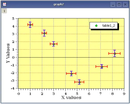
There are several types of curves which can be plotted from a table. They are presented in thePlot menu It is possible to use up to four axes for the data:
In addition to the customizations which have been already been described, for the figure above the axes used for each curve were defined using theCustom CurvesDialog, and two arrows were added with theDraw Arrow. Note that the table must be modified by the addition of a second column of Y data before the second curve can be drawn in the plotting area (usingGraph Menu, and then selecting Add...Add/Remove Curve).
2.1.2
2D plot from function.
There are two ways to obtain such a plot: you can plot a function directly, or fill a table with the values calculated from a function and create the plot in the usual way.
2.1.2.1 Direct plot of a function.
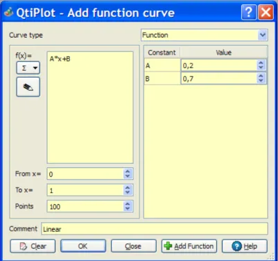
If you just want to plot a function, you can use theNew Function Plot... commandfrom theFile menu, click the icon in the File toolbar, or simply enter Ctrl-F.
This command will open theAdd Function Curve dialog. You can then enter the mathematical expression of your function, the X range to be used for the plot, and the number of points in the X range. Besides classical Y=f(X) functions, you can also define parametric and polar functions.
Figure 2.5: Direct plot of a function.
2.1.2.2 Filling of a table with the values of a function.
If you want to work not only with the plot but also with the resulting data, create a new table as explained in theprevious section. Then fill this table with the values of the function evaluation using theSet Column Values... command.
Let’s obtain the same plot as in the previous example. Create a new table (key Ctrl-T), select the first column and use theSet Column Values... commandeither from the context menu, or theTable menu. The row number can be used in functions by referencing the row number symbol,i. For a range of 0.01-30 in 300 steps (0.01 per step) enter the function expressioni/10and use 300 rows. (Note that since row numbering starts at 1, to actually get the X range used in the last example (0-30 over 300 points), we would need to define the function expression as(i-1)*30/299.)
Figure 2.6: Function plot: filling of the X column.
The second step is to select the second (Y) column and use theSet Column Values... command to set up the function. The expression is a function of the X values (that is the first column) which is namedcol(1). Entersin(col("1"))+cos(col("1")/3+1) as the function and click apply to generate the values in the Y column.
Figure 2.7: Function plot: filling of the Y column.
Once the table is ready, you just have to build the plot as explained in the previous section.
2.2
3D plots
3D plots are generated from data defined as Z=f(X,Y). As with 2D plots, there are two ways to obtain a 3D plot, depending on the way the (X,Y,Z) values are defined:
• You can have your Z values in amatrix. QtiPlot will consider that all the data present in the matrix are Z values, and the X and Y values are defined as functions of the column and row numbers.
The data in the matrix can be entered in several ways: – one by one from the keyboard,
– by reading an ASCII file into a table and converting the table into a matrix, – by setting the values with a function.
• If you want to plot a function, you don’t need a matrix. You can plot a function directly using theNew 3D Surface Plot... command. This will open the correspondingdialog boxwhere you define the mathematical expression of your function. There are several kinds of 3D plots which can be selected, see thePlot 3D menusection of thereference chapterfor a list of the available plots.
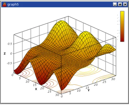
Figure 2.8: Example of a 3D Plots.
3D plots use OpenGL so you can easily rotate, scale and shift them with the mouse. Using the 3D plot settings dialog or the Surface 3D Toolbar, you can change all the predefined settings of a three dimensional plot: grids, scales, axes, title, legend and colors for the different elements.
There are several types of plots which can be built from a matrix. They are presented in thePlot 3D menu
2.2.1
Direct 3D plot from a function
This is the simplest way to obtain a 3d plot. Use theNew 3D Surface Plot... commandfrom the File menuor simply enter Ctrl-Alt-Z. This will open the followingdialog box:
Figure 2.9: Definition of a new surface 3D plot
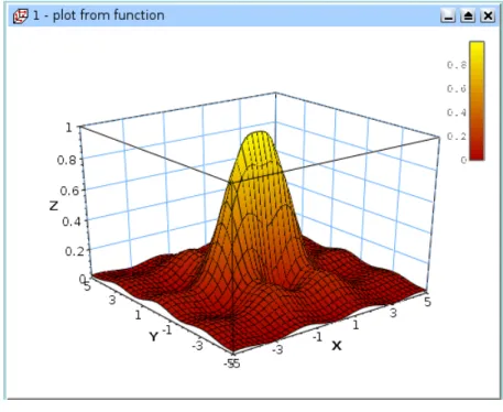
You can enter the function z=f(x,y) and the ranges for X, Y and Z. Then QtiPlot will create a default 3d plot:
Figure 2.10: The 3D surface plot created using defaults
a title, change the colors of the different items, and modify the aspect ratio of the plot. In addition, you can use the commands of the3D plot toolbarto add grids on the walls or to modify the style of the plot. The following plot illustrates some of the possible modifications:
Figure 2.11: The 3D surface plot after customization.
If you want to modify the function itself, you can use thesurface... command which can be activated from the context menu with a right click on the 3D plot. This will re-open thedefine surface function dialog box.
2.2.2
3D plot from a matrix
The second way to obtain a 3D plot is to use amatrix. Therefore, the first step is to fill the matrix. This can be done by evaluation of a function.
TheNew Matrix commandcreate a default empty matrix with 32x32 cells. Then use theSet Dimensions... commandto modify the number of rows and columns of the matrix. Thisdialog boxis also used to define the X and Y ranges.