Medio ambiente y desarrollo

(1)

rade liberalization and

industrial pollution in Brazil

Claudio Ferraz and Carlos E.F.Young

T

S E R

Medio ambiente y desarrollo

23 División de Medio Ambiente y

Asentamientos Humanos

(2)

Economic Research (IPEA) and Santa Úrsula University) and Carlos E.F.Young (Economic Institute, Rio de Janeiro Federal University (IE/UFRJ) wish to acknowledge the valuable research assistance of Sabrina Azamor, Luciana La Rovere and Luisa Schwartzman in the database manipulation and calculations. We would like to thank Ronaldo Seroa da Motta for helpful comments and discussions along the text. Additionally, Claudia Schatan provided useful comments on a previous version. All mistakes remaining are our own.

This document has been reproduced without formal editing. The views expressed herein are those of the authors and do not necessarily reflect the views of the Organization.

United Nations Publications LC/L.1332-P

ISBN: 92-1-121264-2

Printed in United Nations, Santiago, Chile

Applications to the right to reproduce this work are welcome and should be sent to the Secretary of the Publication Board, United Nations Headquarters, New York, N.Y. 1007, USA. Member States and their Governmental Institutions may reproduce this work without prior authorization, but are requested to mention the source and inform the United Nations of such reproduction.

(3)

Index

Abstract I. ... 5

I. Introduction... 7

II. Methodology and Database... 11

A. Methodology... 11

1. The input-output model... 11

2. Introducing emission coefficients ... 12

B. Data Issues ... 13

III. Structural change in the Brazilian industry...15

A. Change in the industrial composition ... 17

B. Impact of the liberalization process on the trade structure. 20 IV. Industrial transformation and pollution... 27

A. Total emissions by category of final demand ... 27

B. Sectoral emission analysis ... 33

Conclusion ... 39

(4)

(5)

Abstract

This paper attempts to estimate the effect of trade liberalization on the industrial structure and pattern of pollution emissions in Brazil. An input-output approach is used to estimate the value of production and potential pollution intensity estimates are undertaken using the industrial pollution projection system. We find that the aggregate intensity of pollutant emission has decreased for the whole industrial sector, but for the export sector, the pollution intensity has been increasing after trade liberalization.

(6)

(7)

I. Introduction

After the debt crisis in the beginning of the eighties and the end of the import substitution strategy era, most Latin American countries have consolidated, in one way or another, programs of structural reforms. For some countries, these reforms were conditioned by international agencies1 and for others, they were accomplished gradually and voluntarily. Among these reforms, trade liberalization had a profound impact on the structure of most economies in the region and Brazil, although a latecomer, was not an exception.

Some of the arguments in favor of market-oriented policy reforms state that economic liberalization reduces static inefficiencies arising from resource misallocation and that economic liberalization enhances learning, technological change, and economic growth.2

Since the late eighties, another crucial point has penetrated the trade liberalization discussions: the environmental consequences associated with freer trade. The theoretical debate over trade and environment is not new,3 but its importance increased substantially with the trade liberalization processes that have been taking place around the world. The hypothesis over the trade and environment link can be divided in two groups. From one side, there exist a possibility that countries with lower environmental standards would develop a comparative advantage in dirty industries. This is associated with the

1

Mainly the IMF and the World Bank.

2 _{Some other arguments widely used in favor of liberalization include the fact that outward-oriented economies are better able to cope}

with adverse external shocks and that market-based economic system are less prone to wasteful rent-seeking activities. See Rodrik (1995).

3

(8)

so called pollution haven hypothesis.4 From another perspective, there exist the possibility that imposing environmental control and regulation in order to avoid the pollution intensive specialization, a country would create additional costs and thus lose competitiveness in world markets.5

Theoretical work done on trade and environment has found an important relationship between trade liberalization and environmental degradation. Models of general equilibrium such as Copeland (1994) and Copeland and Taylor (1994,1995) have shown that, under a wide variety of assumptions, pollution intensity industries tend to migrate to countries with weaker pollution regulations.6 Nevertheless, the empirical work has not validated unambiguously such conclusion. Furthermore, the conclusions that appear from empirical studies on trade and environment are, at most, contradictory.7

As part of the macroeconomic reforms that have been taking place in Brazil during the nineties, trade liberalization is perhaps the one that had larger potential effects on the pattern and structure of industrial production. Since there exist a direct link between the scale of the industrial activity, its composition and pollution emissions, we would like to analyze the possible effects that the trade liberalization process had on the industrial pattern of production and, consequently, on the environment. Furthermore, we want to analyze the link between the pattern of specialization in Brazilian exports after 1990 and the industrial emissions behavior.

Pollution is very hard to measure. There is no single available database in Brazil with a time series of industrial pollution. Consequently, we are going to use the World bank’s Industrial Pollution Projection System (IPPS) that estimates pollution emissions based on output data. Although it does not measure effective pollution (it does not take into account emission’s control), it is an adequate tool to estimate the path that the Brazilian economy took after 1990. Nevertheless, it is important to acknowledge that IPPS coefficients would probably yield a significant upward bias in the emissions estimations.8

The effect of trade liberalization on the environment is usually focused on three effects. Namely the scale effect, the composition effect and the technological effect.9 Here we will concentrate on the scale and composition effect and leave the technological effect aside.10

In order to test our hypothesis, we are going to use input-output methodology to estimate the value of production and then we will apply the IPPS coefficients in order to get estimates of total emissions. These will allow us to undertake two kind of analysis. First we will be able to analyze emissions by the components of final demand. Additionally, we will undertake a disaggregate analysis with 28 industrial sectors in order to study the change in the industrial composition that took place after 1990.

It is important to mention that not all changes in the industry profile that took place in Brazil after 1990 can be attributed to trade liberalization. Nevertheless, it is going to be extremely difficult to separate the different macroeconomic reforms that occurred in Brazil during the nineties in and their direct effects. Industrial profile do not change only due to relative price changes, there are also productivity gains, and for some export oriented industries, there are also gains or losses in competitiveness that can enforce growth.

4

See Low (1992) for a general discussion of trade and environment and Birdsall and Wheeler (1992) for a discussion on this issue for Latin America.

5

See Jaffe et al. (1995) for a study on the effects of environmental regulation on US manufacturing sector’s competitiveness.

6

For other models of trade and environment see Lopez (1994), Chichilnisky (1994) and Ferraz (1997).

7 _{See for example Antweiller, Copeland and Taylor (1998) and Dean (1998).} 8

See Laplate and Smits (1998) for a comparison between real emissions and estimated ones using the IPPS for Latvia.

9

See Antweiller, Copeland and Taylor (1998) for a recent survey and quantification of these three effects for the case of SO2. 10

(9)

The relationship between industrial production and pollution emissions in Brazil was first studied by Carvalho and Ferreira (1992). Using an index of industrial growth, they found that industries with high and average pollution potential grew ate higher rates than the average for the Brazilian industry. Consequently the dynamics of the Brazilian industry since 1980 has been related positively with the level of potential pollution. Nevertheless, their analysis does not incorporate the trade and environment relationship. Seroa da Motta (1993c) studied the link between trade, environment and competitiveness. Using air and water pollution intensity estimates11 and abatement measures for Brazil, he found that most of the sectors considered dirty were also the most dynamic export sectors. Furthermore, comparing potential emissions and actual emissions (after abatement), he found a non negligible difference varying considerably among sectors. This conclusion was also reached by Veiga, Castilho and Ferraz (1995).

A different approach to study the trade and environment link was undertaken by Young (1998c). He used the Seroa da Motta et al. (1993a ;1993b) coefficients and input-output methodology to study the emissions intensity along vectors of final demand for 1985. Young (1999) extended the previous analysis to incorporate the change that took place in the Brazilian export sector from 1985 to 1994. He concluded that the specialization that occurred in the Brazilian industry was intensive in air and water pollution. Although there was a decrease in the emissions intensity for the whole economy, the export complex had higher emission coefficients than the average for the whole period. Furthermore, Young (1999) also compared the decrease in emissions induced trough trade liberalization and found that the total emission induced by export promotion were higher than lower emissions associated with the increase in imports.

The previous results carry out to the analysis of CO2 emissions. Young et al.(1998a, 1998b)

used the COPPE/UFRJ (1998) inventory of CO2 emissions from fossil fuels 12

to obtain emission intensity estimates. He found, as previously, that the export complex had a higher emission intensity than the average for the entire economy. Moreover, there was an increasing trend of the overall emission coefficients in the 1990s, mainly a consequence of the switch in energy sources discussed above.

This paper differs from previous work in its use of input-output methodology and emission coefficients from the IPPS, to perform a sectoral analysis of industrial emissions. This analysis is fundamental to understand what caused the decrease in the emissions intensity of the Brazilian industry as a whole and the increase in the export sector emission intensity.

The paper is structured as follows: section two presents the methodology that is going to be used and the structure of the dataset. Section three analyzes the evolution of the industrial value of production after 1985 and its composition, as well as exports and imports’ structure, together with productivity and unit labor costs. Section four presents our estimates of pollution emissions and section five state our conclusions.

11 _{The database was built using pollution emission and abatement estimates for the year 1988 covering twelve states, and similar}

information for the state of São Paulo for 1991.

12

This inventory was prepared for the Brazilian official representation within the Climate Change Convention. The International Panel on Climate Change (IPCC) established a common methodology for the CO2 estimates at country level.

(10)

(11)

II. Methodology and database

A. Methodology

The methodology adopted in this paper follows the same approach of a series of studies relating economic policies and pollution intensity of the Brazilian industry in terms of local pollutants (Young 1996, 1999) and carbon dioxide (Young et al.1998a,b). There are two new insights in the present exercise, one is that instead of using Brazilian estimates of pollution intensity, we used the IPPS database, estimated according to United States industrial and emissions data. The second additional insight is the analysis of the sectoral evolution of the Brazilian industry and its relation to total emissions.

1. The input-output model

The objective of the input-output model is to describe the sectoral interdependence of the economy, given the current levels of production and consumption. Assuming that all the n sectors of an economy keep a constant share in the market of each product, and that the production processes of all these sectors are technologically interdependent; characterized by a linear relationship between the amount of inputs required and the final output of each sector,13 it is

13

A caveat applies to the use of input-output methodology since it implicitly assumes constant returns to scale. This could be unrealistic for some sectors that present learning by doingandgreat possibilities of increasing returns. Nevertheless, for the case of Brazil, high tech production is still pretty reduced.

(12)

possible to obtain a system containing n equations relating the output of every sector to the output of all other sectors. The model alsoconsiders an autonomous sector (final demand) which is determined exogenously to the model. The sales of each sector should be equal to autonomous consumption (related to the categories of final demand) plus the amount of production destined to the intermediate consumption of all the other sectors (Dorfman, 1954).

Mathematically:

where xij is the amount of output from sector i demanded as intermediate consumption to sector j,

and Ci, Ii, Gi, Ei, Mi and xi are, respectively, the private consumption, investment, public

administration consumption, exports, imports and domestic production of sector i (Prado, 1981). The basic assumption is that the intermediate consumption is a fixed proportion of the total output of each product:

where aij is the technical coefficient determining the amount of product of sector i required for the

production of one unit of product in sector j, and di is the amount of final demand for products from

sector i (di = Ci + Ii + Gi + Ei - Mi). In matrix terms, this is expressed as:

where x is a nx1 vector with the total product of each sector, d is a nx1 vector with sectoral final demand, and A is a nxn matrix with the technical coefficients of production

.

Since the final demand is exogenously determined, the intermediate consumption can be obtained by the following equation:

where (I - A)-1 is the nxn matrix containing the input-output coefficients for the relations between sectors. The same formula is valid for calculating the direct and indirect effects of exports or any other component of the final demand, instead of its aggregate

:

where xf is the nx1 vector containing the total production per sector necessary to obtain the nx1

vector of the f-category of final demand (df). Therefore, the input-output model allows the

determination of the level of economic activity in each productive sector as a function of the final demand for each product.

2. Introducing emission coefficients

The use of extended input-output tables to estimate emissions and other discharges of residuals has become an important instrument to assess environmental problems at the macroeconomic level (for a review, see Førsund, 1985 and Perman et al. 1997; the methodology

x

i

x + C + I + G + Ei - Mi

j=1 n ij i i i =

∑

(1)

d

x

a

=

x

ij j i n j=1 i

∑

.

+

(2)

x = A x + d

₍₃₎

x = (I - A ) d

-1

₍₄₎

f -1 f

x = (I - A ) d

₍₅₎

(13)

adopted in this section is based on Pedersen, 1993). The most common procedure is to assume that emissions are linearly related to the gross output of each sector, in a way that each industry generates residuals in fixed proportions to the sector output. The emission coefficient of pollutant h

by sector i (efhi) can be obtained by dividing the total emission of a sector (emi) by the total output

of the same sector (xi):

Given this assumption, it is possible to obtain the total emission caused by the f-category of final demand through the use of emission coefficients for each sector. In formal terms, this is expressed by

:

where zhf is the nx1 vector containing the total emission of pollutant h per sector associated to the

f-category of final demand, and diag(efh) is the nxn matrix containing in its principal diagonal the

emission factors of pollutant h for each sector, and zeroes elsewhere (Pedersen, 1993).

B. Data Issues

Information of industrial pollution in Brazil is not widely available. Some estimates are available for some specific years, but they do not have a continuity in order for us to undertake a multiple period analysis. Seroa da Motta et al.(1993a) and Seroa da Motta et al. (1993b) have estimates of industrial pollution in Brazil (both air and water pollution) based on 1988 and 1991 data respectively.

As a consequence of the limitations presented above, it would not be possible to use any actual data of industrial pollution in Brazil. Thus we will be using a variable representing the potential pollution of the industry based on the World Bank’s Industrial Pollution Projection System (IPPS).

The IPPS exploits the fact that industrial pollution is heavily affected by the scale of the industrial activity, sectoral composition and technological processes which are employed. Production and emissions data from 200,000 factories in the United States were merged to obtain assessments of sectoral pollution intensity (pollution per unit of activity). Although the estimates based on the IPPS would not be actual emissions, they can be useful as a guideline in order to rank industrial sectors in terms of its potential emissions.14

The IPPS index expresses the pollutant output intensity for six types of air pollutants (SO2, NO2,

CO, VOC, PM10, TP) and three types of water pollution (BOD, TSS and metal). Pollution intensity is expressed as pollutant output divided by total manufacturing. The total manufacturing activity can me measured by many variables, but the main choice is between the value and the output quantity.

Since output can vary in the way it is measured between activities, we chose to use the value of production as our measure of manufacturing activity. The next choice was between using the total value of production or value added by activity. The former was preferred to the latter because energy and material inputs are critical in the determination of industrial pollution. Using value added would exclude the inputs and we would be underestimating the effect of a specific productive activity on pollution emissions.

14

For more detail on the construction of the IPPS database see Hettige et.al. (1994).

hi hi i

ef

=

em

x

₍₆₎

hf h f h -1 f

(14)

Additionally, it is very important to mention that the EPA data used to calculate the IPPS coefficients only cover facilities releasing pollutants over a treshold level of emissions. Consequently, pollution intensities estimated based on these data may be biased. Due to the variability on the industrial sample, there exist a possibility of assigning zero emissions to non-reporting facilities. Additionally, there may exist very pollutant small facilities that do not reach the treshold. Hettige et al. (1994) try to solve this problem presenting inter-quartile estimates which we use in the present study.

The present analysis is undertaken using an input-output methodology. This will allow us to capture backward and forward linkages of the economic activity in the emission of pollutants. Additionally, working with an input-output matrix has another advantage: it will be eliminating the use of imported inputs used in any production process. This is crucial since imported inputs are generating emissions in another country when they are produced and, since we are not working with value added, we would be counting them if we did not decide to use the Leontieff matrix to approximate the value of production.

Due to the form of the Brazilian input-output matrix, we had to aggregate some sectors in order to get our data compatible with the IPPS coefficients. The Brazilian table is near compatible to the ISIC 3 digit classification, although not exactly the same. Consequently we aggregated the data from the IPPS in order to get to the same classification as the Brazilian input-output, ending up with 28 industrial sectors.

The input-output tables from Brazil come from the Brazilian Institute of Geography and Statistics (IBGE) and are available for 1980, 1985 and starting in 1990 they are available annually. Nevertheless, since we wanted to get some comparisons of the structure of production before and after trade liberalization (1990), we included the 1985 matrix in our study. Thus we analyzed data for 1985, 1990, 1993 and 1995. The year of 1993 was picked as a representative period between the year of the liberalization, 1990, and the last year 1995.

The estimation of the value of production in Brazil is quite controversial and we can obtain different results depending the methodology used to calculate it. The recent work by Haguenauer, Markwald and Pourchet (1998), hereafter HMP, compares different results that are obtained using different methodologies. They derived their own estimations based on the 1985 industrial census and obtained results very similar to the ones obtained in Brazilian national accounts. Other methodology that is employed by Moreira and Correa (1997), using the PIA (Pesquisa Industrial Anual) consistently underestimates the value of production.15

Since we are using the Leontieff matrix to estimate the value of production, we would also obtain values that are lower than the ones given by national accounts and by HMP. This is caused by the exclusion of the imported inputs, as mentioned before. The comparison between our estimates of the value of production and HMP can be observed in figure 1.

In order to get the data comparable to other country studies we expressed all our results in 1987 US$ million output value. In order to get the value of production in real terms we used a sectoral deflator for the years that it was available (1990, 1993 and 1995). This was done after analyzing the data using the GDP deflator and noting some problems when same deflator was used for all sectors. Since Brazil had very high rates of inflation in the period prior to 1994, results are very sensitive to the type of deflator that is being used. For the year 1985, we did not have sectoral deflators available and we used the aggregate deflator.

15

See Haguenauer, Markwald and Pourchet (1998) where they compare the results for the value of industrial production in Brazil using different methodologies.

(15)

III. Structural change in the

Brazilian industry

The process of development, as it has been observed in most countries, have followed approximately the same pattern of evolution. These empirical regularities are usually referred as “stylized facts” of the economic growth process.16 The initial predominance of primary production in most countries was followed by a continuous industrialization process. Syrquin and Chenery (1986) accounts this transformation estimating that the predicted share of primary production in a country with $300 GDP per capita would be 44% compared to a 12% in manufacturing. Nevertheless, as output per capita increases to $4000, these shares would change to 16% in primary production and 24% in manufacturing.

As income per capita increases, the industry share in national output tends to decline in favor of a growing service sector. In developed countries, the service sector corresponds to more than 50% of the national product. This tendency is also taking place in developing countries. In Brazil, the share of industry in the beginning of the century represented approximately 10% of the GDP while agriculture represented 38%.17 Between 1945 and 1950, the share of industry increased above the share in agriculture, although the share of other sectors (including services) remained basically constant. The share of industry grew to a maximum of 28% in 1970. It remained

16

See Kaldor (1961) .

17

(16)

relatively stable until 1980 when it started to decrease with a substantial increase in the service sector of the Brazilian economy. In 1990 the share of industry in GDP corresponded to a 24%. This pattern of evolution is consistent with the inverted-U model for manufacturing share in national output first described by Kuznets (1965).

The second characteristic of the development process is the change in the industrial composition. During the industrialization process, the composition of manufacturing changed significantly, shifting from a predominant light manufacturing to a prevailing heavy industry.18 This process was accentuated in countries that were rich in natural resources because of the relative high price of labor in relation to capital.

In Brazil the sectoral industry composition changed considerably. Bonelli (1996a) analyzed this transformation dividing the industrial sectors in traditional (oldest industries such as non-durable consumption goods, textiles and food products), dynamic-A (intermediate modern goods) and dynamic-B (capital goods and consumption durable goods), the first group decreases its importance from 79,65% in 1940 to 39,06% in 1990. At the same time, the dynamic A and B increase consistently its importance peaking in a 43,1% and 17,82% respectively in 1990.

This pattern of evolution inside the industrial structure, follows the tendency proposed by Syrquin (1989). The evolution from light to heavy industry can also be interpreted as the change from a predominant traditional sector to a dynamic sector that represents most of the heavy industry.

The pattern of development described above has direct implications for the pattern of pollution emissions. Since there exists a direct relationship between industrial output and emissions, if the industrial sector has a tendency to increase its share of participation in GDP, there is a direct tendency of increasing the pollution emissions. This is the so called the scale effect. Additionally, as it has been mentioned above, the structure within the industrial sector changes along the development path. There is a gradual transformation of light industry into heavy industry, which are, in general, more intensive in emissions. This effect is known in the literature as the composition effect.19

Besides, technology gets better and cleaner through time. The costs of pollution control falls over time and as countries grow, they tend to adopt cleaner technology. This effect is called the technological effect and it is the most difficult one to measure.20 In this paper we will concentrate on the first two since we do not have data available to measure technological change in the control of emissions.

The three effects described above tend to generate an inverse-U shaped curve for emissions as a function of income per capita. Pollution will first increase with the development process (with GDP per capita) and then pollution decrease as GDP per capita increases. This relationship is known in the literature as the environmental Kuznets curve and although some econometric studies have found this relationship in cross section data, there is a widespread controversy over its generalized existence.

18

The difference between light and heavy industry is rather arbitrary. Here we are using the Chenery, Robinson and Syrquin (1986) definition; light industry includes food and consumer goods and heavy industry includes producer goods and machinery.

19

See Birdsall and Wheeler (1992) for a discussion of these different effects.

20

See Eaton and Kortum (1997) and Rodríguez-Clare (1996) for some studies on the role of international trade on technology diffusion.

(17)

A. Change in the Industrial Composition

The pattern of evolution that took place in the Brazilian industry until 1990 was presented above. Nevertheless since 1989 and more drastically since 1990, Brazil has been consolidating its trade liberalization process. This structural change, along with other macroeconomic reforms, modified the industrial structure, as well as the productivity and the industrial production growth. Consequently the pattern of potential pollution emissions suffered a substantial effect.

The first task in order to analyze the consequences of trade liberalization in the Brazilian industrial emissions pattern is to study its scale effects. Although we know that the changes that occurred after 1990 were not only due to trade liberalization, we can assume that the change in relative prices and resource allocation that occurred due to the liberalization process played an important and prominent role.

As it was explained above, we used input-output tables in order to estimate the value of industrial production (VP) in Brazil. Since we needed a baseline year in order to compare it to the post-liberalization industrial production, we chose 1985. As it was mentioned before, this was due to the fact that input-output tables for Brazil where not available between 1986-1989. Nevertheless, we compared our estimates to Haguenauer, Markwald and Pourchet (1998) in order to understand what happened to the value of production in the Brazilian industry between 1986 and 1989. This comparison can be observed below in figure 1.

Figure 1

VALUE OF INDUSTRIAL PRODUCTION IN BRAZIL: 1985-1995

Source: Haguenauer, Markwald and Pouchet (1998) and authors’ calculations based on IBGE data

0 50000 100000 150000 200000 250000 300000 350000 400000 450000 500000 1985 1986 1987 1988 1989 1990 1991 1992 1993 1994 1995 Year Million of $

(18)

It is important to note the significant differences between our estimates of the value of industrial production and HMP estimates. These differences are due, firstly, because using the input-output approach to calculate VP, we exclude imported inputs of production. Consequently, we would expect our estimates of the VP to be lower than HMP.

Taking the VP in million of dollars (in nominal terms), we can analyze its evolution from 1985 to 1995. There is a consistent increase in its value between 1985 and 1990. This increase is consistent with the growth of GDP during the same period. It represents a 107,1 % increase if analyzed using the HMP estimates and a 70,1% using our estimates. After 1990, due to the recession, the value of production decreased significantly reaching a minimum in 1992 and increasing consistently again until 1995. Therefore, the years chosen to analyze the industry evolution (1985, 1990, 1993 and 1995) are representative of the business cycle that occurred from 1985 to 1995.

In real terms, using our data from VP based on 1987 US$, the VP decreased from 1985 to 1990 by 3.3 %. Nevertheless, starting in 1990, there is a consistent increase in the value of production. From 1990 to 1993, the increase was 2.63% and from 1993 to 1995 real VP increased by 5.41%. Consequently, in terms of the scale effect, the value of production in real terms increased between 1990 and 1995 by 8.18% creating a significant scale effect and consequently a possible increase in total emissions associated with the increment in the industrial activity.

Although the effect of an increase in the industrial VP is important, the relative shift in the composition of manufacturing is crucial in order to determine what happened to industrial pollution after 1990. We need to understand if the growth in the value of production is due to relative cleaner or dirtier activities.

The first way to analyze these changes is comparing the relative weight of different sectors in the 1990 VP and the corresponding value in 1995.

Based on our estimates of the total value of production, we can observe in table 1 the sectors that gained more in terms of participation in the total value of production.

Comparing to the share in the 1985 industrial VP, the sectors that had substantial increases in their industrial VP share were: other food products (includes beverages), motor vehicles; meat industry; and electronic equipment. On the other hand, the main losers during the same period of time were: textiles; coffee industry; iron and steel; and petroleum refinery.

If we take the base year as 1990 and we do the same exercise, we find that the main winners based on our estimates were: motor vehicles; meat industry; other food products and electronic equipment. On the other hand, the sectors that lost most in terms of their shares in the VP were: non-metallic minerals; textiles; and petroleum refinery.

Another important issue is the evolution of the shares prior to the liberalization

process. Were there sectors that were losing their share due to other factors prior to 1990? Between 1985 and 1990 the main change in the composition of the VP was due to other food products; non-metallic minerals; electronic equipment; meat industry; electric material. The main losers in the same period were petroleum refinery; coffee; iron and steel.

Consequently, many of the sectors that are losers as a whole for the period 1990-95, were already suffering considerable losses in their importance in the total value of industrial production even before the trade liberalization process. Consequently, we can propose that not all the change that took place after 1990 were due only to trade liberalization. There were many macro and micro economic changes that occurred in the Brazilian economy during the eighties that decreased the incentive for some of these sectors. The trade liberalization process, probably just accentuated a process that was already taking place with the end of the II PND.

(19)

Table 1

SECTOR PARTICIPATION IN THE TOTAL VALUE OF INDUSTRIAL PRODUCTION 1987 US$ MILLION

(%)

Activity Code Activity Description 1985 1990 1993 1995

04 Non-metallic Minerals 3,36 4,00 3,57 3,30

05 Iron and Steel 7,01 5,64 6,05 5,60

06 Non-ferrous metallurgic 2,50 2,48 2,20 2,43

07 Other metallurgic 4,65 4,79 4,59 4,66

08 Machinery and Equipment 6,10 6,07 5,69 5,76

10 Electric Material 2,71 3,22 2,98 3,42

11 Electronic Equipment 2,92 3,53 2,95 4,23

12 Motor vehicles 2,96 3,14 3,69 4,48

13 Vehicle parts and Other vehicles 4,56 4,26 4,40 4,60

14 Wood and Furniture 2,84 3,12 2,85 2,75

15 Pulp, Paper and Paperboard 4,15 4,62 4,44 4,79

16 Rubber Industry 1,59 1,58 1,65 1,58

17 Chemical Industry 2,87 2,81 3,25 2,81

18 Petroleum Refineries 12,35 11,40 12,77 10,18

19 Other Chemical products 3,95 4,09 3,97 3,69

20 Pharmacy and Veterinary Products 2,11 2,25 2,36 2,49

21 Plastic Products 1,84 2,16 1,94 1,94

22 Textiles 5,89 5,73 5,04 4,74

23 Wearing Apparel 3,30 3,20 2,70 2,71

24 Footwear 1,96 1,83 1,81 1,49

25 Coffee Industry 2,25 0,99 0,97 0,87

26 Other Vegetable Products 3,84 3,77 4,00 4,09

27 Meat Industry 3,13 3,73 4,23 4,58

28 Dairy Products 1,49 1,76 1,69 1,74

29 Sugar Factories and Refineries 1,41 1,14 1,17 1,38

30 Vegetable Oils 2,65 2,16 2,32 2,47

31 Other Food Products 4,02 4,84 5,01 5,57

32 Other Industries 1,57 1,70 1,70 1,65

Source: Author’s calculations based on IBGE data

We can compare our results to another study that analyzed the change in the industrial composition after 1990. Bonelli and Gonçalves (1998) used averages over the following aggregation of periods, 1985/1989, 1990/92 and 1993/1996, in order to describe the main changes that took place after 1985. They found that the sectors that had the major losses in participation were clothing and wearing apparel, textiles, footwear, and machinery.

On the other hand, they point out that a small group of industries gained importance in the industrial VP. This group included beverages (included in our aggregation as other alimentary products), perfumes, soap and candles (included in our aggregation as pharmaceutical and veterinary products) and tobacco (included in our classification as vegetal products).

Our results are quite different from Bonelli and Gonçalves (1998). This is due to three reasons: firstly because they are using averages over some periods. Secondly, they are using data

(20)

from the Industrial Monthly Survey (PIM) instead of data from national accounts.21 Thirdly, their aggregation is different from ours.22

B. Impact of the Liberalization Process on the Trade Structure

Any trade liberalization process is aimed at correcting price distortions in order to allocate resources efficiently and promote long run growth. It is usually argued that opening up an economy will increase welfare because it will create an increase in the variety and quantity of goods available for consumers, and at the same time, it will create additional static and dynamic effects related to increases in productivity and burst in exports in the medium and long run.23

To analyze the penetration of imports and the increase in exports by sectors in Brazil, we are going to analyze the evolution of import penetration24 and export coefficients. We used coefficients that were calculated by Haguenauer, Markwald and Pourchet (1998) using their estimates of the value of production.25

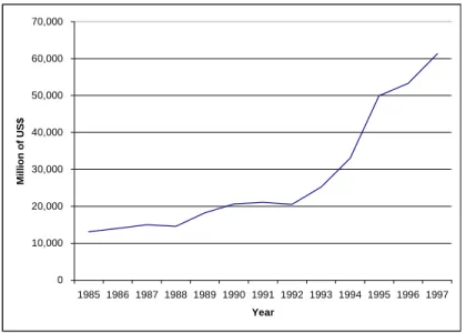
The value of Brazilian imports increased consistently since 1990 as it can be observed in figure 2. Although the penetration of imports in the economy as a whole increased substantially after 1990, the real change took place after 1993. The aggregate industrial import penetration coefficient changed, from 7.9, in 1993 to 10.7, in 1995. Nevertheless this change was not symmetric across all sectors. In table 2 we can observe how the import penetration coefficient changed across sectors.

Figure 2

VALUE OF BRAZILIAN IMPORTS: 1985 – 1997

Source: authors’ calculations based on Funcex data

21 _{Since our methodology needed input-output tables, we could not use yearly data, as it was already mentioned. Nevertheless, VP}

estimates based on the Industrial Monthly Survey (PIM) face many criticisms. See Haguenauer, Markwald and Pourchet (1998) for more details.

22

An alternative approach was used by Moreira and Correa (1997) based on Valdes (1992). They used a potential output methodology to analyze the change in the composition of the industrial structure in Brazil after 1989.

23 _{Assuming that the real exchange rate will not be overvalued.} 24

Imports/ Apparent consumption.

25

Although coefficients calculated by Moreira and Correa (1997) are also available, we preferred HMP due to their VP estimations and also because their aggregation is similar to ours.

0 10,000 20,000 30,000 40,000 50,000 60,000 70,000 1985 1986 1987 1988 1989 1990 1991 1992 1993 1994 1995 1996 1997 Year Million of US$

(21)

Table 2

SECTORAL IMPORT PENETRATION COEFFICIENTS: 1985-1995

(Falta unidad de medida)

Activity Code

Activity Description 1985 1989 1990 1991 1992 1993 1994 1995

04 Non-metallic Minerals 1 0.9 0.9 1.2 1.2 1.3 1.5 2

05 Iron and Steel 1.2 2.4 1.8 3.1 2.4 1.8 1.7 2.4

06 Non-ferrous metallurgic 6.1 9 7.5 11.5 14.2 4.4 14.3 18.8

07 Other metallurgic 1.2 1.6 1.9 2.9 2.5 3.2 3 4.5

08 Machinery and Equipment 7 6.2 8.3 13.5 13.8 12.5 14 19.1

10 Electric Material 8 7.9 6.5 10.4 12.8 14.8 17.5 18.8

11 Electronic Equipment 12.1 12.4 10 15.9 24 27.6 29.9 33.2

12 Motor vehicles 0.1 0 0.2 1.7 2.9 5.6 9 14.2

13 Vehicle parts and Other vehicles 14.8 8 7.4 11.9 12.9 12.3 13.4 13.4

14 Wood and Furniture 0.7 0.5 0.4 0.4 0.5 0.7 0.7 0.9

15 Pulp, Paper and Paperboard 1.7 2.5 2.2 3.3 2.4 2.7 3.4 6.4

16 Rubber Industry 3.4 6.1 5 6.6 5.1 5 6.4 9

17 Chemical Industry 11.8 17.7 16.9 22.9 21.1 22.9 23.9 29.1

18 Petroleum Refineries 3 3.5 3 5 5 7.4 6.7 9.3

19 Other Chemical products 5.9 6.6 5.3 7.4 8.3 9.4 9.4 10

20 Pharmacy and Veterinary Products 4.2 4.2 3.8 5.5 4.4 4.7 5.9 6.8

21 Plastic Products 0.6 0.6 0.8 1.2 1.5 1.8 2.1 3.2

22 Textiles 0.7 2.5 2.4 4.3 4.8 9.7 9.7 13.3

23 Wearing Apparel 0.1 0.2 0.4 0.6 0.5 0.5 1.2 3.2

24 Footwear 3.3 7.3 5.8 11.5 13.4 12 10.5 15.9

25 Coffee Industry n.a.

26 Other Vegetable Products 13 3.5 3.8 6.4 6.4 8 7.5 7.8

27 Meat Industry 1.4 5.7 3.9 2.4 2.4 1.5 2.3 2.8

28 Dairy Products 0.7 4.7 2 2.9 1.1 1.9 2.8 4.7

29 Sugar Factories and Refineries n.a.

30 Vegetable Oils 2.8 1.9 1.2 2.6 3 4.2 7.9 6.9

31 Other Food Products 1.6 2.6 2.5 2.6 2.2 2.4 2.6 4.4

32 Other Industries 11.5 13.1 12.2 15.9 17.9 16.1 16.5 22.1

Source: MHP (1998)

The main changes took place in the electronic equipment sector followed by the chemical industry, motor vehicles and electric material. Although the more impressive growth was in motor vehicles if compared to the 1990, other sectors also had a high growth rate greater than 200% between 1990 and 1995. These sectors included including wearing apparel; textiles; vegetable oils; plastic products; electronic equipment; and petroleum refineries.

Exports were directly affected through the trade liberalization process as well. This change is usually explained by many factors including the decrease in the cost of imported inputs; the possibility of accessing new technologies and the need for an increase in productivity due to the imported products competition.

In aggregate terms, the value of exports grew continuously after 1992 as it can be observed in figure 3. Nevertheless, its performance was negatively influenced by the appreciation of the real exchange rate after 1993 and also by the changes in productivity and unit labor costs.

(22)

Figure 3

VALUE OF BRAZILIAN EXPORTS: 1985 - 1996

Source: authors’ calculations based on Funcex data

One way to measure the export performance is analyzing the evolution of the export coefficient.26 In aggregate terms the export coefficient did not increase after trade liberalization in 1990 and although it increased to an impressive 12.2% in 1992, it decreased to 9.9% in 1995. This was due mainly to the more than proportional increase in the industrial value of production after 1993. Therefore there is no significant upward trend in the aggregate export coefficient after 1990.

The aggregate export performance after 1990 was definitely influenced by three effects. First the effective real exchange rate increased until 1990, but has decreased consistently since then creating a negative incentive for exports.27 Second the unit labor cost increased after 1992 with an increase of 30% until 1995 and even tough there was an increase in productivity, it was not enough to compensate the prior two negative effects.28

Nevertheless, the relative performance across sectors was not homogeneous. Based on table 3, it is possible to analyze what happened to each industrial sector exports after 1990.

Based on the previous table, the sectors that had a high export coefficient (higher than 30%) in 1995 were non-ferrous metallurgic, footwear, sugar and refineries, and vegetable oils. Furthermore, the higher rates of growth in the coefficient took place in sugar and refineries; followed by electric material; wood and furniture; and machinery and equipment.

The lowest growth rate in the export coefficient took place in iron and steel; petroleum refineries; other food products, other vegetable products; and motor vehicles, all of them with negative growth rates varying from –9.2 % in iron and steel to –25% in the motor vehicles sector.

26 _{Defined as exports/value of production.}

27 _{According to Moreira and Correia (1997) it reached 120 in July, 1992 and decreased consistently to a level around 70}

and 80 in October 1995.

28 _{The productivity and unit labor cost effect are going to be explored further in sectoral terms in the next section.}

0 10,000 20,000 30,000 40,000 50,000 60,000 1985 1986 1987 1988 1989 1990 1991 1992 1993 1994 1995 1996 Year Million of US$

(23)

Table 3

SECTORAL EXPORT COEFFICIENTS: 1985-1995

Activity Code Activity Description 1985 1989 1990 1991 1992 1993 1994 1995

4 Non-metallic Minerals 2.9 1.9 1.4 2 2.3 2.8 2.4 2.3

5 Iron and Steel 16.1 20.5 16.3 26.5 21.8 19.5 15.6 14.8

6 Non-ferrous metallurgic 12.1 22.5 20.6 30.4 37.6 34.3 31.6 31.3

7 Other metallurgic 4.4 4.3 4.2 6.7 7 7 6.1 5.4

8 Machinery and Equipment 7.5 5 4 7.1 9.2 9 8.9 8.2

10 Electric Material 7 8.7 6.3 12.4 17.6 19.3 16.7 15.3

11 Electronic Equipment 11.1 7.8 4.6 8 12.1 10.3 8.3 6.6

12 Motor vehicles 14.1 12.8 6.4 7.5 13.2 9.4 7.7 4.8

13 Vehicle parts and Other vehicles 21.2 15.1 12.3 18.6 20.3 17.7 15.8 13.1

14 Wood and Furniture 7.8 3.6 3.1 4.9 7.5 8.7 8.8 7.4

15 Pulp. Paper and Paperboard 7.8 8.2 7.2 9.4 10.5 9.9 11.1 12.4

16 Rubber Industry 8 8.4 7.2 10.9 10.7 9.3 8.5 8

17 Chemical Industry 6.4 9 7.4 9.7 11.3 11 9 11

18 Petroleum Refineries 10.9 6.1 4.2 4.3 4.1 3.9 4.3 3.8

19 Other Chemical products 2.5 3.2 2.4 3.6 4 4.4 4 4.5

20 Pharmacy and Veterinary Products

21 Plastic Products

22 Textiles 8.3 7.5 6.7 10.8 13.4 11 10.1 10

23 Wearing Apparel

24 Footwear 32 26.7 29.6 46.5 61 55.9 45.4 46.5

25 Coffee Industry

26 Other Vegetable Products 24.3 14.4 13.7 12.8 15.8 13.4 12.5 11.8

27 Meat Industry 17.6 9.7 7.1 12 17.7 18.7 14.8 12.9

28 Dairy Products

29 Sugar Factories and Refineries 14.9 14.2 17.3 17.4 22 30.4 27.4 50.4

30 Vegetable Oils 43.1 41.2 34.1 32.4 37.6 38.1 47.6 42.8

31 Other Food Products 5.2 2.8 2.5 2.8 3.4 3.3 2.7 2.2

32 Other Industries 14.4 8.8 8 11.1 14.8 12.8 10.7 9.1

Source: MHP (1998)

In terms of the participation in the total value of exports, the top five industrial sectors in 1990 were iron and steel; vehicle parts and other vehicles; other vegetable products; vegetable oils; petroleum refineries, each one representing above 5% of the total export value. In 1995, this distribution did not change considerably. The top five sectors in terms of share in total exports were iron and steel; vegetable oils, vehicle parts and other vehicles; pulp, paper and paperboard; coffee; other vegetable products; machinery and equipment and non-ferrous metals; all of them corresponding to more than 5%. The most important increase in participation was the pulp, paper and paperboard sector; followed by machinery and equipment and non-ferrous metals.

Although the growth rate in the value of Brazilian exports between 1990 and 1995 was 47.1%, some sectors had growth rates well above that. The sectors that had higher growth rates in the value of its exports were sugar factories and refineries; wood and furniture; pulp, paper and paperboard; meat industry; other chemical industry; machinery and equipment; rubber industry; and non-metallic minerals. All of them with growth rates superior to 100%.

(24)

Whereas some sectors intensive in natural resources still constitute in 1995 an important share of Brazilian exports, after the decrease in the incentives, sectors like electric material, transport material increase their relative participation in the export profile.

The performance of each industrial sector, was directly affected by the productivity change in the Brazilian industry after 1990.29 Although there is a great controversy in trying to measure the gains in productivity that occurred after 1990, there is widespread evidence suggesting an increase in productivity for the Brazilian industry as a whole.30 If on one hand the productivity in the industrial sector was stagnated from 1985 to 1991, it started growing in 1992 and from 1993 on it increased consistently with high growth rates. The annual average growth in productivity from 1990 to 1996 was 8% (Salm et al, 1997). This increase was consistent independently of the business cycle; recession during 1991 and 1992; prosperity during 1994 and 1995 and back to recession in 1993. After 1993 the industry starts to grow again and without any retrieval in the industrial employment. This resulted in an excellent productivity growth (Salm et al. 1997).

In sectoral terms, Electrical material and communication was the sector with highest productivity growth between 1990 and 1995 with a growth rate of 74%. It was followed by transport equipment with a 49.3 % increase; pulp, paper and paperboard with a 48.6% and non-metallic minerals with a 41.3% increase. The productivity growth across sectors can be observed in table 4.

Table 4

PRODUCTIVITY GROWTH IN THE BRAZILIAN INDUSTRY FOR SELECTED SECTORS: 1990-95

(%)

Industrial category 1990-95 Growth

Non-Metallic Minerals 41,3

Metallurgy 36,2

Mechanical 36,7

Electric and Communications Material 74,0

Transport Equipment 49,3

Paper and Paperboard 48,6

Rubber Industry 29,4

Chemical Industry 37,4

Plastic Products 34,8

Textiles 35,1

Wearing Apparel 21,5

Food Products and Beverages 37,4

Source: Salm, Saboia and Carvalho (1997)

It is interesting to observe that sectors that had highest gains in terms of participation in the total value of production also had very high gains in productivity. Electronic equipment and transport equipment are clear examples. At the same time, these were sectors that were lost significant their share in total exports (Veiga, 1994).

In a more desegregated analysis done by Bonelli and Fonseca (1998), they categorized industrial sectors according to their average productivity and average unit labor cost growth between 1990-1996. We present their results in table 5 below.

29 _{For further evidence on the trade liberalization and productivity relationship fpr Brazil see Hay (1997).}

30 _{See Salm, Saboia and Carvalho (1997) for a good survey. See also Bonelli (1996b) and Considera (1998) for different}

(25)

Table 5

AVERAGE UNIT LABOR COST AND AVERAGE PRODUCTIVITY GROWTH IN THE BRAZILIAN INDUSTRY: 1990-1996

(%)

Activity Description Unit cost of labor 1990-96 average growth Productivity of labor 1990-96 average growth Non-metallic Minerals 1.5 8.9 Non-ferrous metallurgic 1.4 6.9 Machinery 5.4 6.3

Electric material and Communication -1.5 12.0

Transport material -1.4 10.4

Wood 9.1 5.0

Furniture 5.2 7.4

Paper and Paperboard 2.1 8.3

Rubber 1.9 7.5

Leather and Skin 13.9 -0.2

Chemical 3.1 7.8

Pharmacy 11.5 0.9

Candles. Soaps and Perfumes 5.2 4.5

Plastic Material Products -0.6 8.3

Textiles 0 8.5

Made-up Textile Goods. Footwear and Textile Articles 1.8 6.9

Food Products 2.4 7.0

Beverages 3.7 8.2

Tobacco 6.2 7.0

Source: Bonelli and Fonseca (1998)

Although the aggregation in the previous table is different from the one we used, we can observe clearly which sectors had highest productivity and unit labor cost growth. In terms of productivity, the main winners were leather and skin, followed by pharmacy; wood products; tobacco; and machinery products. In general, sectors that had high ULC growth had lower labor productivity gains.

Furthermore, sectors that had higher ULC growth lost significant competitiveness during the nineties. The main losers were electric material and communication; transport materials; non-metallic minerals, and textiles.

(26)

(27)

IV. Industrial transformation and

pollution

The pattern of pollution emissions in Brazil is estimated using the value of production and the IPPS coefficients. Our analysis is done in two different and complementary ways. First we study aggregate emissions for each pollutant and analyze how each category of final demand (e.g. consumption, exports) contributed to final emissions. Secondly, we analyze the evolution of sectoral emissions and link this to the pattern of structural change that occurred in Brazil after 1990.

A. Total emissions by category of final

demand

The estimated emission of pollutants required in the production chain resulting from each category of final demand are presented in table 6. Note that these results do not necessarily reflect actual emissions, since the emission coefficients were not obtained from field surveys in Brazil. The possible bias generated by this problem is discussed further below.

(28)

Table 6

ESTIMATED TOTAL AIR POLLUTION EMISSIONS FOR BRAZIL

(kg)

Pollutant Investment* Exports Public administration Private consumption Total SO2 1985 85,208,280 51,456,452 11,208,534 132,522,553 289,149,318 1990 97,727,498 37,021,336 13,431,767 144,393,174 291,194,567 1993 82,702,458 50,542,486 17,681,100 135,672,173 290,518,096 1995 75,823,414 48,092,314 15,898,302 133,660,623 283,115,062 CO 1985 17,001,647 17,740,536 2,267,169 26,811,574 65,734,687 1990 15,686,859 13,476,706 2,599,503 27,983,866 58,663,040 1993 13,009,422 19,009,613 3,248,248 25,196,857 61,513,944 1995 13,636,876 17,044,278 3,039,404 26,200,866 61,521,054 NO2 1985 60,227,102 33,198,794 6,750,998 88,012,044 193,867,505 1990 68,975,919 24,090,394 8,198,599 95,851,107 196,026,901 1993 58,448,045 33,698,929 10,861,275 90,678,809 195,498,593 1995 53,898,608 32,328,364 9,663,374 89,852,561 191,744,687 VOC 1985 32,756,862 29,712,014 4,978,079 78,565,378 149,861,714 1990 34,772,929 20,910,742 6,042,885 87,956,005 147,653,314 1993 27,584,043 30,029,227 8,314,373 81,708,261 153,123,792 1995 30,683,620 25,128,544 7,214,845 86,838,288 155,261,152 Particulate Total 1985 31,940,457 18,319,236 2,419,188 42,245,825 97,701,293 1990 35,405,177 14,157,636 3,016,697 45,311,147 97,043,893 1993 29,745,645 19,849,580 3,949,401 42,894,714 97,017,168 1995 28,202,041 18,945,619 3,512,747 44,854,554 97,900,760 Metal 1985 242,805 243,579 19,020 377,154 910,193 1990 221,070 223,378 23,398 393,137 837,210 1993 167,862 285,820 26,668 325,731 823,733 1995 196,225 253,619 23,754 360,322 862,958

Source: Authors’ calculations based on IBGE data dan IPPS coefficients. * Changes in stocks were not included

Based on our estimates, the pollutants that have the highest contribution to total emissions are: SO2, NO2 and VOC. Nevertheless, the two greatest contributors have decreased their emissions

after 1990. Other pollutants, although with lowest total contributions, have increased significantly its total potential pollution: CO, VOC and metals (air). In terms of water potential pollution, both BOD and TSS have increased its total emissions after 1990, nevertheless, metals (water) have decreased substantially its total emissions. Consequently, there is not an overall trend that total emissions are following after 1990.

(29)

Table 7

ESTIMATED TOTAL WATER POLLUTION EMISSIONS FOR BRAZIL

(kg)

Pollutant Investment* Exports Public administration Private consumption Total BOD 1985 1,877,066 4,139,547 2,387,478 14,826,848 24,058,359 1990 2,044,634 3,629,284 2,636,128 15,752,959 23,855,449 1993 1,401,824 5,273,680 3,292,082 14,006,453 23,820,047 1995 1,603,663 6,489,825 3,389,471 14,998,026 26,797,125 TSS 1985 3,221,830 5,532,352 2,432,525 16,877,620 29,181,052 1990 3,290,097 4,689,468 2,706,321 18,309,722 28,798,015 1993 2,446,495 6,400,034 3,384,040 16,340,861 28,856,885 1995 2,699,334 6,659,685 3,426,015 17,584,954 30,998,369 Metal 1985 12,981 32,520 7,408 152,276 215,428 1990 13,700 27,022 8,735 158,629 207,285 1993 9,197 34,897 11,127 130,564 191,505 1995 9,164 29,989 10,598 137,354 193,030

Source: authors’ calculations based on IBGE data and IPPS coefficients

It is important to analyze together with total emissions, the contribution of each final demand category to total output. This can be observed in table 8.

Table 8

DOMESTIC INDUSTRIAL OUTPUT REQUIRED BY FINAL DEMAND CATEGORIES

(% of total industrial output)

Year Investment* Exports Public administration Private consumption

1985 20.4 14.2 10.9 51.5

1990 20.6 9.8 15.5 54.5

1993 17.0 12.4 17.5 51.7

1995 17.5 10.3 16.1 54.2

*

Changes in stocks were not included

Comparing the previous table with tables 9 and 10, we can observe that the contribution of each final demand category to total emissions does not follow their contribution to the aggregate output.

(30)

Table 9

AIR EMISSIONS BY CATEGORIES RELATIVE TO THE TOTAL

(%)

Pollutant Investment* Exports Public administration Private consumption SO2 1985 29.5 17.8 3.9 45.8 1990 33.6 12.7 4.6 49.6 1993 28.5 17.4 6.1 46.7 1995 26.8 17.0 5.6 47.2 CO 1985 25.9 27.0 3.4 40.8 1990 26.7 23.0 4.4 47.7 1993 21.1 30.9 5.3 41.0 1995 22.2 27.7 4.9 42.6 NO2 1985 31.1 17.1 3.5 45.4 1990 35.2 12.3 4.2 48.9 1993 29.9 17.2 5.6 46.4 1995 28.1 16.9 5.0 46.9 VOC 1985 21.9 19.8 3.3 52.4 1990 23.6 14.2 4.1 59.6 1993 18.0 19.6 5.4 53.4 1995 19.8 16.2 4.6 55.9 TP 1985 32.7 18.8 2.5 43.2 1990 36.5 14.6 3.1 46.7 1993 30.7 20.5 4.1 44.2 1995 28.8 19.4 3.6 45.8 Metal 1985 26.7 26.8 2.1 41.4 1990 26.4 26.7 2.8 47.0 1993 20.4 34.7 3.2 39.5 1995 22.7 29.4 2.8 41.8

Source: Authors’ calculations based on IBGE data and IPPS coefficients

Our estimates show that the contribution of the export complex to total emissions, for each pollutant, is higher than its share on total output. This is a strong indication that the export complex presents a higher than average pollution intensity, i.e. the ratio between the total emission and the value of production of each category of final demand is higher for exports than for other categories. This can be seen in tables 11 and 12, which presents total pollution intensity estimates.

(31)

Table 10

WATER EMISSIONS BY CATEGORIES RELATIVE TO THE TOTAL

Percentage

Pollutant Investment* Exports Public administration Private consumption BOD 1985 7.8 17.2 9.9 61.6 1990 8.6 15.2 11.1 66.0 1993 5.9 22.1 13.8 58.8 1995 6.0 24.2 12.6 56.0 TSS 1985 11.0 19.0 8.3 57.8 1990 11.4 16.3 9.4 63.6 1993 8.5 22.2 11.7 56.6 1995 8.7 21.5 11.1 56.7 Continues Metal 1985 6.0 15.1 3.4 70.7 1990 6.6 13.0 4.2 76.5 1993 4.8 18.2 5.8 68.2 1995 4.7 15.5 5.5 71.2

Source: authors’ calculations based on IBGE data and IPPS coefficients

* _{Changes in stocks were not included}

The results show there has been an overall improvement in the total emission coefficients from 1990 to 1995. Nevertheless, it also shows that this improvement was already taking place prior to 1990, as it can be observed by analyzing the change in the total emissions coefficient from 1985 to 1990. Consequently this relative improvement can not be attributed directly to the trade liberalization process that took place during the nineties. Nevertheless, although these coefficient has been decreasing for the economy as a whole, they have been increasing for most pollutants in the export sector.

This problem is particularly important for metals (air), CO and TSS, but the amount of emission required to produce one unit of export related output exceeds the average of the economy for every pollutant. Moreover, the intensity of pollution is higher in export related activities than in any other group for the 9 parameters in 1995. In 1985 the investment complex was the most intensive in NO2, SO2 and total particulate air emissions. This has been reverted during the nineties

given the higher growth in emissions intensity in the export complex. Furthermore, only one parameter (VOC) showed a declining emission intensity in the 1985/95 period in deep contrast with the rest of the economy. This is an indication that the overall change in the industrial composition has created potential benefits in cleaner activities for the Brazilian economy as a whole. Nevertheless, the output directly or indirectly destined to external markets has presented the opposite trend. There has been a potential specialization toward “dirty” industries.

(32)

Table 11

EMISSION INTENSITY OF AIR POLLUTION BY CATEGORY OF FINAL DEMAND

(kg/1987US$ million)

Pollutant Investment* Exports Public administration Private consumption Total SO2 1985 912 794 224 562 632 1990 942 751 173 525 578 1993 925 776 193 499 554 1995 761 821 175 434 499 CO 1985 182 274 45 114 144 1990 151 273 33 102 116 1993 146 292 35 93 117 1995 137 291 33 85 108 NO2 1985 645 512 135 373 424 1990 665 489 105 348 389 1993 654 518 118 334 373 1995 541 552 106 292 338 VOC 1985 351 459 100 333 327 1990 335 424 78 320 293 1993 309 461 91 301 292 1995 308 429 79 282 274 PT 1985 342 283 48 179 214 1990 341 287 39 165 193 1993 333 305 43 158 185 1995 283 324 39 146 173 Metal 1985 2.60 3.76 0.38 1.60 1.99 1990 2.13 4.53 0.30 1.43 1.66 1993 1.88 4.39 0.29 1.20 1.57 1995 1.97 4.33 0.26 1.17 1.52

*

(33)

Table 12

EMISSION INTENSITY OF WATER POLLUTION BY CATEGORY OF FINAL DEMAND

(kg/1987US$ million)

Pollutant Investment* Exports Public administration Private consumption Total BOD 1985 20.1 63.9 47.7 62.9 52.6 1990 19.7 73.6 33.8 57.3 47.3 1993 15.7 81.0 35.8 51.6 45.4 1995 16.1 110.8 37.1 48.7 47.2 TSS 1985 34.5 85.4 48.6 71.6 63.8 1990 31.7 95.1 34.7 66.6 57.1 1993 27.4 98.3 36.8 60.2 55.0 1995 27.1 113.7 37.5 57.1 54.6 Metal 1985 0.139 0.502 0.148 0.646 0.471 1990 0.132 0.548 0.112 0.577 0.411 1993 0.103 0.536 0.121 0.481 0.365 1995 0.092 0.512 0.116 0.446 0.340

B. Sectoral emission analysis

In order to comprehend the composition effect that took place in the Brazilian industry after 1990, it is necessary to undertake a sectoral emission’s analysis. In tables 13 and 14 we present the relative contribution of the main pollutant sectors to total emissions from 1985 to 1995.

As it can be observed above, non metallic minerals represents the highest contribution to total emissions for SO2, NO2, PT and Metals. Moreover, its contribution to total emissions has been

slightly increasing over time. For CO emissions, Iron and steel is by far the largest contributor, with its share varying from 44.6% in 1985 to 39.8% in 1995. Iron and steel is also an important contributor to PT and Metal emissions. For VOC emissions, petroleum refinery is the largest contributor to total emissions. Nevertheless, its contribution has also been decreasing over time falling from 31% in 1985 to 25% in 1995.

Based on the previous table, we can observe that, in general, the highest air polluting sectors are: non metallic minerals; petroleum refineries; iron and steel; Pulp, paper and paperboard; textiles and chemical industry; wood and furniture; and sugar factories and refineries. 31

31

This result is probably distorted by the fact that the IPPS classification includes alcohol together with sugar, while IBGE considers them separately (alcohol for fuel is classified in the chemical industry).

(34)

Table 13

INDUSTRIAL AIR POLLUTION: SECTORS WITH HIGHEST CONTRIBUTIONS TO TOTAL EMISSION

Percentage

1985 1990 1993 1995

SO2

Non metallic minerals 35.8% 40.8% 37.5% 37.5%

Petroleum refineries 24.4% 21.6% 24.9% 21.5%

Pulp, paper and paperboard 10.7% 11.4% 11.3% 13,2%

Textiles 13.7% 12.8% 11.6% 11.8%

Chemical industry 4.7% 4.4% 5.2% 4.9%

CO

Iron and steel 44.6% 38.9% 40.8% 39.8%

Pulp, paper and paperboard 11.0% 13.2% 12.4% 14.1%

Wood and furniture 10.8% 12.8% 11.5% 11.7%

Sugar factories and refineries 6.4% 5.6% 5.7% 7.0%

NO2

Textiles 10.9% 10.1% 9.2% 9.3%

VOC

Other food products 6.7% 8.0% 8.2% 9.4%

Other metallurgic 8.9% 8.9% 8.5% 9.0%

PT

Iron and steel 10.7% 8.4% 9.2% 8.9%

Metals

Iron and steel 28.1% 23.9% 26.6% 24.8%

Textiles 19.0% 19.5% 17.8% 16.9%

Other metallurgic 5.2% 5.6% 5.6% 5.7%

Source: authors’ calculations based on IBGE data and IPPS coefficients

Water pollution estimates are presented in the following table and there is some slight variation from air pollution in relation to the main polluting sectors.

(35)

Table 14

INDUSTRIAL WATER POLLUTION: SECTORS WITH HIGHEST CONTRIBUTIONS TO TOTAL EMISSION

Percentage

1985 1990 1993 1995

BOD

Pulp. Paper and paperboard 58.5% 63.6% 62.8% 63.5%

Textiles 12.9% 12.3% 11.1% 9.8%

Vegetable oils 3.4% 2.7% 3.0% 3.0%

TSS

Textiles 19.9% 19.0% 17.1% 15.8%

Iron and steel 7.2% 5.7% 6.2% 5.7%

Vegetable oils 5.1% 4.1% 4.5% 4.7%

Metals

Textiles 39.3% 37.6% 34.7% 33.0%

Iron and steel 6.5% 5.1% 5.8% 5.4%

Pulp, paper and paperboard is by far the most polluting sector. Its contribution to total pollution varies from approximately 60% on BOD to 50% on TSS and 45% on Metals. Furthermore, for all three pollution measures, its contribution to total emissions have been increasing from 1985 to 1995. Other important water pollutant sectors are textiles, iron and steel and petroleum refineries. Vegetable oils, although less important, also represents a considerable contribution to total emissions of BOD and TSS.

For the economy as a whole, it has been observed that the pollution intensity in the Brazilian industry has decreased after 1985 and specially after 1990. Nevertheless, the pollution intensity of the export sector has increased for most pollutants. This was caused by the fact that high growth sectors were not the most pollutant ones. On the contrary, relatively clean sectors had highest growth rates after trade liberalization. Motor vehicles, for example, with a 47.8% growth rate and the coffee industry with a 35% growth rate, are clear examples of this pattern.32 On the other hand, the sectors that gained most in the export markets were the dirtiest sectors.

These results can be observed in table 15 where we present the growth rate of the total value of industrial production and exports from 1990 to

1995.

32

The IPPS data do not present a coefficient for the coffee industry; therefore it was considered in this study with a zero-emission coefficient (which is not true in reality). Anyway, the coffee industry is not characterized by a high emission intensity.