Probability Distribution of Return and Volatility in Crude Oil Market
Dr. Tung-Li Shih, Assistant Professor, Department of Hospitality Management,MingDao University, Taiwan
Dr. Hai-Chin Yu, Professor, Department of International Business, Chung Yuan Christian University, Taiwan
ABSTRACT
Using probability distribution techniques, this paper explores the statistical properties in returns and volatility of crude oil market. After fitting the daily returns from January 1, 1986 to December 31, 2007 into probability distributions and estimating the parameters of the Gaussian distribution, we find that crude oil market shows a positive return, slightly left-skewed and lepto-kurtosis. After estimating the peak and width of the volatility of the log-normal distribution, the crude oil market is an unstable and volatile market. All these findings are important to market traders and hedging strategies.
Keywords: Probability Distribution, Return, Volatility, Crude Oil Market
INTRODUCTION
Crude oil is the world economy’s most important source of energy and is critical to economic growth. Crude oil prices, associated with bouts of inflation and economic instability over the last 30 years, have been rising in recent years. Sharp oil prices changes, either increases or decreases, may reduce aggregate output temporarily because they delay business investment by raising uncertainty.
The volatility of commodity prices creates uncertainty, and therefore an unstable economy during the past decade for both energy-exporting and energy-importing countries. Higher crude oil prices result in an increase in inflation and a subsequent recession, as crude oil prices are negatively correlated to economic activities (Ferderer, 1996). High crude oil price is an increasing risk to global economic growth; high crude oil price will squeeze global growth. Most recessions were preceded by oil price shocks, i.e. 1974 (The Yom Kippur War started with an attack on Israel by Syria and Egypt on October 5, 1973), 1980(Events in Iran and Iraq led to another round of crude oil price increases in 1979 and 1980), and 1990(The price of crude oil spiked in 1990 due to the Iraqi invasion of Kuwait and the Gulf War) economic recessions in the United States (Huntington, 1998).
Recent years have seen the commodities complex enjoy an impressive bull run. Oil (about US$21 per barrel in beginning of 2002 raised up to US$120 per barrel in beginning of 2008), commodities, metals and gold (about US$278 per ounce in beginning of 2002 went up to US$1000 per ounce in beginning of 2008) prices are continuing soaring. Crude oil is part of the commodities market and crude oil prices are subject to large fluctuation in times of over or under-supply. The cycle of crude oil market price can extend over a number of years. Besides, crude oil price and the crude oil market are affected by global demand which is intensely affected by economic and political conditions. Crude oil price history can be linked to macroeconomic history. Thus, it is great importance to analyze probability distribution of returns and volatility for crude oil market.
Financial market volatility is important to the theory and practice of asset pricing, asset allocation and risk management. Volatility has been learned either by fitting parametric econometric models such as generalized autoregressive conditional heteroscedasticity (GARCH), by studying volatilities implied by options prices in conjunction with specific option pricing models such as Black-Scholes, or by studying direct indicators of volatility such as ex post squared or absolute returns. In this article, we analyze market volatilities for crude oil market. Market volatility is estimated using average local price changes, to extract more information from time series of volatility, this work uses the statistical measurements of probability distribution function.
In this paper, we apply modern time series techniques to detect daily crude oil market. This paper focuses on the crude oil price of West Texas Intermediate (WTI), which trades on the New York Mercantile Exchange (NYMEX). Crude oil is not only the most actively traded commodity, but also the largest volume of features trading of any physical commodities. Owing to its excellent liquidity and price transparency, crude oil contracts serve as an important international pricing benchmark.
This study is different from the extant literature in a number of ways. First, we use the methodology of probability distributions to analyze the returns and volatility in crude oil market. Second, based on the symmetric and bell-shaped characteristics of the return distribution, we fit the return distribution into Gaussian function and then estimate the parameters (the peak and width of the distribution) in the distribution. Third, based on the asymmetric and right-skewed characteristics of the volatility distribution, we use the log normal distribution to fit the volatility distribution, and calculate the parameters (the peak and width of the distribution, the volatility area for the three markets) of the distribution. The remaining sections are organized as follows. Section 2 presents the literature review. Section 3 shows the data description and the probability distributions of return and volatility in crude oil market. Finally, section 4 concludes.
LITERATURE REVIEW
This study is motivated by the fact that most empirical articles focus on high frequency data of stock returns to derive their empirical regularities. Gopikrishnan et al. (1999) did a detailed analysis of the distribution of returns for S&P 500 index, NIKKEI index and Hang-Seng index, for time intervals ranging from 1 minute to one month, and found that the distribution of returns is consistent with a power-law asymptotic behavior. Yu and Huang (2004) examined the statistical properties of volatility among New York, Tokyo, Taiwan, South Korea, Singapore, and Hong Kong markets. Chiang et al. (2009) investigated the phase distribution and phase correlation of Dow Jones Industry Average (DJIA) and NASDAQ high-frequency intraday data. Both the DJIA and NASDAQ index changes satisfy the Levy distributions. Ng (2000) constructed a volatility spillover model to examine the magnitude and changing nature of volatility spillovers from Japan (Tokyo Stock Price Index) and to the US (Standard and Poor’s 500 Index) to six Pacific-Basin equity markets (including Hong Kong, Korea, Malaysia, Singapore, Taiwan, Thailand).
Recently, Chiang et al. (2009) studies the high-frequency intraday returns and volatilities of DJIA and NASDAQ indices using probability distribution techniques. They found that both NASDAQ and DJIA have excessively high returns at opening intervals, although the NASDAQ has a higher return than DJIA. The higher returns in NASDAQ are associated with higher volatilities across all the intervals in each trading day. Yu et al. (2008) using the probability distribution techniques, they explore whether any differences exist in returns and volatility of yen/dollar spot markets among different time zones at Tokyo, London, and New York. It is found that New York shows the highest return, followed by London, and Tokyo, which has a negative return with a long left tail. And Tokyo is found to have the lowest volatility in the log normal distribution while London and New York show similar volatility distributions, implying similar investor risk-return preference behavior between London and NY markets.
But few empirical studies focus on physical commodities. Liew and Brooks (1998) measure the determinants of daily returns and volatility in the Kuala Lumpur crude palm oil futures market using ARCH/GARCH techniques to model the time varying behavior of returns and volatility over the period 1980 to 1994. They find significant evidence of month and open interest effects in returns and also find strong evidence of daily, monthly, yearly, volume and open interest effects in volatility when ARCH/GARCH models are used to estimate volatility. Plourde and Watkin (1998) found that crude oil price volatility during 1985-1994 was higher than price volatility for nine other commodity (includes gold) price volatility. Pindyck (1999) analyized oil, coal, and natural gas price changes during 1870-1996, but did not compare their volatilities, and he calculated a constant volatility measure over a very long period during which volatility is believed to have changed. Recently, Tabak and Cajueiro (2007) analyze the efficiency of Brent and West Texas Intermediate crude oil markets by means of estimating the structure of these time series. They test for time-varying degrees of long-range dependence and find evidence that crude oil market has become more efficient over time.
DATA
Our data consists of time series of daily prices of crude oil market, the West Texas Intermediate crude oil price was chosen to represent the oil spot market. The trading data is extracted from AREMOS for the period 1 January 19861 to 31 December 2007. In order not to confound our statistical inference, we removed several fixed holidays, including Christmas (December 24-26), New Year’s (December 31-January 2), and July Fourth. We also cut Easter Monday, Memorial Day, and Labor Day, as well as Thanksgiving and the day after. Although our cuts do not capture all the holiday market slowdowns, they do succeed in eliminating the most important such daily calendar effects. All in all, we were left with a total of 5,405 observations, for the construction of our daily returns and volatilities.
The interactions between the different elements, such as the traders and the assets, comprising financial markets generate many observations, such as transaction price, the share volume traded, the trading frequency, and the values of market index. Figure 1 displays the raw data from the representative market.
The Price Movement of Crude Oil Market
Time U S D pe r ounc e 1986 1988 1990 1992 1994 1996 1998 2000 2002 2004 2006 10 20 30 40 50 60 70 80 90 100
Figure 1: The price movement for the West Texas Intermediate crude oil market
Changes in oil prices have been associated with major developments in the world economy, and are often seen as a trigger for inflation and recession. The increases in oil prices in 1974 and then again in 1979 were important factors in producing a slowdown in the world economy at a time when inflation was rising. (Barrell and Pomerantz, 2004) The price of crude oil price spikes in 1990 with uncertainty associated with Iraq’s invasion of Kuwait. The price spike was substantial, within weeks of August 1990; Saudi light the crude oil price had jumped from about $15 per barrel to over $33 per barrel. But the impact on oil supplies was negligible, not least because Saudi Arabia and other Arabia countries were allied with US forces and they made efforts to counteract the price increase. Once it was clear that the US was committed to expelling Iraq, prices began to slide. (Kubarych, 2005).
In the wake of the Asian financial crisis and a pick-up of Iraqi oil sales under the United Nations oil-for-food program, oil prices plummeted to $10 per barrel in late 1998. Global demand began to swell as the high-tech bubble encouraged a big investment boom in North America and Europe and as the Asian economies began to recover. By the middle of 2000, oil prices tripled. It represented a sharper price advance than during the shock of the Iranian revolution. The eventual peaking in the oil price coincided with President Clinton’s decision to sell crude oil from the Strategic Petroleum Reserve. The tripling of crude oil prices early 2002 has had generally more muted and often paradoxical effects on the financial markets. (Kubarych, 2005) Recently, there is higher demand in industrialized countries and China’s rapidly expanding economy has created a huge demand boost. The strategies adopted by the Organization of Petroleum Exporting Countries (OPEC) also affect the crude oil price. (Yang et al., 2002; Wirl and Kujundzic, 2004; Horan et al., 2004) Hedge funds and other speculators betting on the possibility of higher prices have exacerbated price pressure in the market. In addition to that the world’s major oil customers dependent on the Middle East for their oil. The violence in Iraq and Saudi Arabia has raised fears about an interruption to supplies.
1
International transactions of crude oil and petroleum products entered the age of the market with the sudden drop in oil prices, due to the start of netback sales by Saudi Arabia in 1986.
The crude oil price has climbed up steadily recently, the crude oil price reached about $70 per barrel in April 2006. At the start of 2007, crude oil price reflected a steady decline that had begun from July 2006, decreasing from a high slightly more than $75 per barrel to about $51 per barrel. A number of factors contributed to the decline. These included mild weather and rising heating oil and gasoline inventories in the United States. By the fall of 2007, increased speculation in commodity markets, in conjunction with the devaluation of the U.S. dollar and new geopolitical concerns, crude oil prices rose to over $90 per barrel. By November 2007, crude oil price was testing the $100 per barrel mark, peaking at $99.29 in the third week of November. Crude oil price remain volatile through 2008 due to geopolitical risks, Organization for Economic Corporation and Development inventory tightness, and worldwide refining bottlenecks.
Table 1: Some important events that affect the crude oil price
Time Event Price Movement
August, 1990 Iraq’s invasion of Kuwait, the Gulf War about $15 per barrel to over $33 per barrel
December, 1998 In the wake of the Asian financial crisis and a pick-up of Iraqi oil sales under the United Nations oil-for-food program
oil prices plummeted to $10 per barrel
Early 2002 Higher demand in industrialized countries and BRICs has created a huge demand boost. The strategies adopted by the OPEC also affect the crude oil price.
about $21 per barrel in beginning of 2002
At the start of 2007 Decreasing from a high slightly
more than $75 per barrel to about $51 per barrel.
MEASURE RETURN AND THE PROBABILITY DISTRIBUTION OF RETURN
To explicitly display the distribution of daily return, this section builds the probability distributions corresponding to the entire trading time of daily return.
Quantify the Returns
A number of studies investigated the time series of returns on varying time scales
t
in order to probe the nature of the stochastic process underlying it. (Gopikrishnan et al., 1999; Yu and Huang, 2004; Choi and Hammoudeh , 2009) To construct the time series of returns using the time series of the daily crude oil priceZ t
( )
, the price changeR t
( )
is defined as the change in the logarithm of the daily crude oil price,
ln
ln
R t
Z t
t
Z t
(1)where
t
denotes the time interval of sampling with
t
1
day in the data.We first examine the time series of daily returns for crude oil market shown in Figure 2. The maximum and minimum returns are 0.4367 and -0.4035 may suggest the presence of sharp discontinuities in the series; it can be easily seen in Figure 2. -.3 -.2 -.1 .0 .1 .2 .3 86 88 90 92 94 96 98 00 02 04 06
Figure 2: The daily time series returns for the West Texas Intermediate crude oil market Probability Distribution of Return
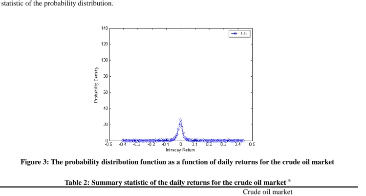
To display the probability distribution of daily returns more clearly, we will construct the probability distribution for the time series of daily returns. To construct the probability distribution, we adopt the histogram method and group the total samples into 100 intervals. Then, we count the number of daily return ranging between each interval. Figure 3 shows the probability distribution of daily returns for the sampling market. And Table 2 represents the preliminary statistic of the probability distribution.
Figure 3: The probability distribution function as a function of daily returns for the crude oil market
Table 2: Summary statistic of the daily returns for the crude oil market a Crude oil market
Mean 0.0244 (0.5364) Max 0.4367 Min -0.4035 Standard Dev. 0.0290 Skewness b -0.0115 (0.7294) Kurtosis b 37.9153** (0.0000) Jarque-Bera c 323692.99** (0.0000)
a. The table summaries the daily returns distribution for the West Texas Intermediate crude oil market. The sample covers the period from January 1, 1986 through December 31, 2007 for a total of 5,405 observations.
b. Under the null hypothesis of independent, identically distributed normally distributed returns, the sample Skewness and Kurtosis are asymptotically normal with means of 0 and 3.
c. Jarque-Bera is Jarque-Bera test statistic, distributed
22. d. ** denotes significance at 0.05.From Figure 3 and Table 2, the average return of crude oil market is 0.0244 with a standard deviation of 0.0290. The distribution is slightly left-skewed (with a Skewness of -0.0115) and Lepto-kurtosis distribution (with a Kurtosis of 37.9153), implying negative returns occur more often than positive returns in crude oil market. Clearly, the Jarque-Bera test statistic and its corresponding p-value which is significant at 0.05 showing that the null hypothesis of a normal distribution is rejected. This evidence is rational and consistent with Lee and Cheng (2007)2 and Choi and Hammoudeh (2009)3. However, daily returns in crude oil market have significant kurtosis parameters meaning that it exists in fat tails.
2 Lee and Cheng (2007) found that the WTI crude oil returns show negative skewness (-1.0977) and leptokurtic (20.4882) from 2 June 1986 to 29
October 2004 with a total of 4,574 observations.
3
Choi and Hammoudeh (2009) studied that the WTI crude oil returns show negative skewness (-1.0448) and leptokurtic (20.5755) from 2 January 1986 to 19 July 2005.
The sample mean of the crude oil market appreciation of 0.0434% is indistinguishable from zero at standard significance levels given the sample standard deviation of 3.0023%4. However, the returns of the crude oil market are clearly not normally distributed, for example the sample kurtosis of 37.9153 is highly statistically significant.
In order to further analyze the characteristics of the probability distributions, we choose the Gaussian function5 to fit original daily returns. Daily returns show an almost symmetric and bell-shaped surface that conforms to characteristics of the Gaussian function. The results are consistent with earlier work by Yu et al. (2008). The Gaussian function is defined as
2 0 2 2/ 2
R R w oA
f R
y
e
w
(2)where
y
0 is baseline,R
0 is the center of the peak,A
is the total areas under the curve from the baseline, andw
is equal to the width of the peak at half height. The fitted probability distributions and corresponding parameters of the daily returns for the crude oil market is shown in Figures 4 and Table 3.
Figure 4: The fitted probability distribution of daily return for entire trading time for West Texas Intermediate crude oil market
Table 3: The parameters of daily returns fitted by the Gaussian function a,b
Parameters Crude oil market
Mean(μ) 0.0244
Standard Dev.(σ) 0.0290
Center(
R
0) -0.0028Width(
w
) 0.0323Height(
h
) 21.983a. We use the Gaussian function to fit the original distribution. The Gaussian function is
2 0 2 2( ) 0 ( ) / 2 R R w A f R y e w , where 0
y
is the baseline,R
0is the center of the peak,w
is equal to the width of the peak at half height, andh
is the height of the fitted distribution. b. The sample covers the period from January 1, 1986 through December 31, 2007 for a total of 5,405 observations.Figure 4 shows the probability distribution of the daily returns for the crude oil market with a peak at -0.0002. Here, the peak means the location of the highest probability of daily returns, and it also represents daily returns in crude oil market are more central at 0. Table 3 shows the parameters of daily returns fitted by the Gaussian function. The crude oil market has a negative center at -0.0028. In addition, the width of the crude oil market is 0.0323. This evidence
4 Assuming the returns to be uncorrelated, the standard deviation for the mean equals the standard deviation divided by the root of the sample size.
(Andersen and Bollerslev, 1997)
5
Gaussian function is characteristic symmetric bell sharp curve that quickly falls off towards plus/ minus infinty. The parameter of Gaussian function is the height of the curve’s peak, the position of the center of the peak, and the width of the bell.
is rational and consistent; it shows that crude oil market is more volatile and easy to be shocked by imbalance of supply and demand, policies adopted by the OPEC, political tensions in the Middle East and so on. This finding is in agreement with Regnier (2007) showing that since the 1973 oil crisis, crude oil prices have been more volatile than other commodities and Yang et al., (2002) that given the 4% cut in OPEC production, the crude oil prices are expected to increase unless the recession is serve, Rigobon and Sack (2005) found evidence that oil prices are affected by conflict (war) risk, and Lee and Cheng (2007) demonstrated that the volatility of crude oil is of significantly high levels during periods of the Gulf War.
MEASURE VOLATILITY AND THE PROBABILITY DISTRIBUTION OF VOLATILITY
To explicitly display the distribution of the daily return volatility, this section builds the probability distributions corresponding to the entire trading time of daily return volatility.
Quantify Volatility
This study estimates volatility as the local average of absolute price changes over a proper time interval T. Generally, T is an adjustable parameter, but this study takes
T
5
days6 for constructing the time series of volatility. The volatilityV t
( )
is defined as the average of absolute value ofG t
( )
over a time windowT
5
t
,
4
01
5
nV t
G t
n t
(3)Figure 5 shows the calculated time series of volatility for the crude oil market. It is a volatile market with a highest mean (at 0.0178) and standard deviation (at 0.0138). Crude oil prices volatility, associated with bouts of inflation and economic instability over the last twenty years, its volatility fluctuates most dramatically over the daily cycle. It reveals a pronounced difference in the volatility over the day, ranging from a low of around 0.0006 to a high of around 0.1798. This pattern is closely linked to the market activity in the various financial centers around the globe. Guo and Kliesen (2005) indicated that unanticipated economic developments could roil crude oil markets and increase volatility, and the decline in the trade-weighted value of the US dollar. Another cause of increased uncertainty could reflect exogenous events that are noneconomic in nature, such as the strategies of the OPEC or political instabilities in the Middle East. Lee and Cheng (2007) the prices of crude oil are often subject to variables of supply, demand, production economics, environmental regulations and other factors.
.00 .01 .02 .03 .04 .05 .06 .07 .08 86 88 90 92 94 96 98 00 02 04 06
Figure 5: The time series of volatility for the crude oil market
Probability Distribution of Volatility
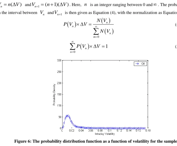
To display the distribution of volatility more clearly, we will construct the probability distributions for the time series of volatility. The resultant distributions for the sample markets are observed to have long tails and be asymmetrical across the peak of the curve. The log-normal distribution can take characteristics into consideration, and thus the log-normal distribution function is used to fit the data. To construct the probability distribution of volatility, this
6 Since the absolute value of daily return during a week with 5 observations, we set a time window which is equal to 5; therefore, the daily volatility
study uses the histogram method to count the value of volatility
N V
(
n)
for the volatility ranging between(
)
n
V
n
V
andV
n1
(
n
1)(
V
)
. Here,n
is an integer ranging between 0 and
. The probability of volatilityin the interval between
V
n andV
n1 is then given as Equation (4), with the normalization as Equation (5).
0 n n n mN V
P V
V
N V
(4)
01
n nP V
V
(5)Figure 6: The probability distribution function as a function of volatility for the sample market
Table 4: Summary statistic of the volatility of daily returns for crude oil market a Crude oil market
Mean 0.0178** (0.0000) Max 0.1798 Min 0.000645 Standard Dev. 0.0138 Skewness b 4.1299** (0.0000) Kurtosis b 31.0909** (0.0000) Jarque-Bera c 232845.89** (0.0000)
a. The table summaries the distribution of the daily volatilities for the crude West Texas Intermediate oil market. Market volatility is estimated using average local price changes. The sample covers the period from January 1, 1986 through December 31, 2007, for a total of 5,405 observations. b. Under the null hypothesis of independent, identically distributed normally distributed returns, the sample Skewness and Kurtosis are asymptotically
normal with means of 0 and 3.
c. Jarque-Bera is Jarque-Bera test statistic, distributed
22. d. ** denotes significance at 0.05.Figure 6 represents the result of probability distribution of volatility. First, the distribution is asymmetric with the peak, and second, the distributions have longer tails than the normal distribution. The results are consistent with earlier work by Yu and Huang (2004), and Yu et al. (2008). From the distributions shown in Figure 6, some descriptive statistics for the sample markets are listed in Table 4. The average volatility of crude oil market is 0.0178 with a standard deviation of 0.0138. The distribution is right-skewed (with a Skewness of 4.1299) and lepto-kurtosis distribution (with a Kurtosis of 31.0909). It shows that the typical non-normality of financial time series.
2 1/ 2 21
1
exp
ln
2
2
cV
P V
w
V
wV
(6)
0P V dV
1
(7)Yu et al. (2008), and Yu and Huang (2004) suggest that the log-normal distribution may capture features. According to their methodology, we adopt the log-normal function P(V) and the function contains two parameters, the first Vc represents the scale parameter, the secondωrepresents distribution width. The corresponding values of the two parameters are listed in Table 5. It not only shows the highest probability and the width of the distribution, but also shows the average volatility, indicating the whole volatility, and the standard deviations, indicating the fluctuations in volatility.
Table 5: The parameters of volatility of log-normal function for the crude oil market Crude oil market
Mean 0.0178
Standard Dev. 0.0138
Peak Probability a 0.0147
Dis. Width a 0.5999
Volatility Area
V
c
w
-0.5852~0.6146a. The equation (6) contains two parameters, the first is peak probability represents the peak probability location, and the second is distribution width the represents distribution width.
2 1/ 2 21
1
exp
ln
2
2
cV
P V
w
V
wV
From Table 5, as for the crude oil market, it possesses the peak probability and peak width, at 0.0147 and 0.5999, respectively. Meanwhile, given that the range of
V
c
w
represents typical volatility conditions in sampling market, the “volatility area” in crude oil market is -0.5852~0.6146.CONCLUSIONS
Crude oil is not only the world’s most actively traded commodity, but also the largest volume of futures trading of a physical commodity in the world. This article is different from the existing works; we apply time series techniques to detect commodities markets to find out the statistical properties of daily returns and volatility. In this article, we offer a comprehensive study of the daily returns and volatility process for universally recognized and widely traded physical assets: crude oil market. Using probability distribution techniques, this paper explores whether any probability distribution differences exist in returns and volatility of crude oil market. This can avoid potential biases resulting from only seeing the mean, standard deviation of returns and neglecting the other parameters of the distribution (the peak and width of the distribution, the volatility area for the sampling market). And we can get more information about the investors' behaviors.
All these findings are important to market traders and hedging strategies, these have important implications for international investors, multinational firms, and risk managers and so on. They consider the impact of commodity return and volatility on portfolio diversification and on management, risk assessment, pricing and hedging, asset allocation decisions.
After fitting the distributions and estimating the parameters of the Gaussian distribution for daily returns, we find that the average return for crude oil market is 0.0244, with a standard deviation of 0.0290. The distribution is slightly left-skewed (with a skewness of -0.0115) and lepto-kurtosis (with a kurtosis of 37.9153). This evidence is rational and consistent with Lee and Cheng, 2007; Choi and Hammoudeh, 2009. After estimating the peak and width of the volatility for the log-normal distribution, the crude oil market is a unstable and volatile market. This evidence is rational and
consistent with Regnier, 2007; Yang et al., 2002; Rigobon and Sack, 2005; Lee and Cheng, 2007; Guo and Kliesen, 2005; because crude oil market is more volatile and easy to be shocked by the imbalance of supply and demand, the policies adopted by the OPEC, the political tensions in Middle East and so on.
REFERENCES
Andersen, T.G. and Bollerslev T. (1997). Intraday periodicity and volatility persistence in financial market. Journal of Financial Economics, 4, 115-158.
Barrell, R. and Pomerantz O. (2004). Oil prices and the world economy, NIESR Discussion Paper 242.
Chiang, T. C. Yu, H.C. and Wu, M.C. (2009), Statistical properties, dynamic conditional correlation and scaling analysis: Evidence from Dow Jones and NASDAQ high-frequency data, Physica A: Statistical Mechanics and its Applications, 388(8), 1555-1570.
Choi, K. and Hammoudeh, S. (2009). Long memory in oil and refined products markets, The Energy Journal, 30(2), 97-116. Ferderer, J.P. (1996). Oil price volatility and the macro economy. Journal of Macroeconomics, 18, 1-26.
Gopikrishnan, P. Plerou V. Amaral Luı´s A. N. Meyer M. and Stanley H. E. (1999). Scaling of the distribution of fluctuations of financial market indices. Physical Review E, 60(5), 5305-5316.
Guo, H. and Kliesen K.L. (2005). Oil price volatility and U.S. macroeconomics activity, Federal Reserve Bank of St. Louis Review, 87(6), 669-683. Horan, S.M. Peterson J.H. and Mahar. J. (2004). Implied volatility of oil futures options surrounding OPEC meetings, The Energy Journal, 25(3),
103-125.
Huntington, H.G. (1998). Crude oil prices and US economic performance: where does the asymmetry reside? Economic Journal, 19(4), 107-132. Kubarych, R. (2005). How oil shocks affect markets, The International Economy, 19(3), 32-36.
Lee, M.C. and Cheng W.H., 2007, Correlated Jumps in Crude Oil and Gasoline During the Gulf War, Atlantic Economic Journal, 39, 903-913. Liew, K.Y. and Brooks R. D. (1998). Returns and volatility in the Kuala Lumpur crude palm oil futures market, The Journal of Futures Markets, 18(8),
985–999.
Ng, A. (2000). Volatility spillover effects from Japan and the US to the Pacific–Basin, Journal of International Money and Finance, 19, 207–233. Pindyck, R.S. (1999). The long-run evolution of energy prices, The Energy Journal, 20(2), 1-27.
Plourde, A. and Watkins, G. (1998). Crude oil prices between 1985 and 1994: how volatile in relation to other commodities? Resource and Energy Economics, 20(32), 245-262.
Regnier, E. (2007). Oil and energy price volatility, Energy Economics, 29, 405-427.
Rigobon, R. and Sack, B. (2005). The effect of war on US financial markets, Journal of Banking and Finance, 29, 1769-1789.
Tabak, B.M. and Cajueiro D.O. (2007). Are the crude oil markets becoming weakly efficient over time? A test for time-varying long-range dependence in prices and volatility, Energy Economics, 29(1), 28-36.
Wirl, F. and Kujundzic, A. (2004). The impact of OPEC conference outcomes on world oil prices 1984-2001, The Energy Journal, 25(1), 45-62. Yang, C.W. Hwang, M.J. and Huang, B.N. (2002). An analysis of factors affecting price volatility of the US Oil market, Energy Economics, 24,
107-119.
Yu, H. C. and Huang, M.C. (2004). Statistical properties of volatility in fractal dimension and probability distribution among six stock markets, Applied Financial Economics, 14, 1-9.
Yu, H. C. and Chiou, I., and James J. W. (2008). Does the weekday effect of the Yen/Dollar spot rates exist in Tokyo, London, and New York? An analysis of panel probability distributions, Applied Economics, 40, 2631-2643.