Sensitivity analysis of longitudinal binary data
with non-monotone missing values
PASCAL MININI
Laboratoire GlaxoSmithKline, Unit´e M´ethodologie et Biostatistique, 100 route de Versailles, 78163 Marly le Roi, France, and INSERM U472, 16 avenue Paul Vaillant-Couturier, 94807 Villejuif, France
MICHEL CHAVANCE∗
INSERM U472, 16 avenue Paul Vaillant-Couturier, 94807 Villejuif, France
SUMMARY
This paper highlights the consequences of incomplete observations in the analysis of longitudinal binary data, in particular non-monotone missing data patterns. Sensitivity analysis is advocated and a method is proposed based on a log–linear model. A sensitivity parameter that represents the relationship between the response mechanism and the missing data mechanism is introduced. It is shown that although this parameter is identifiable, its estimation is highly questionable. A far better approach is to consider a range of plausible values and to estimate the parameters of interest conditionally upon each value of the sensitivity parameter. This allows us to assess the sensitivity of study’s conclusion to assumptions regarding the missing data mechanism. The method is applied to a randomized clinical trial comparing the efficacy of two treatment regimens in patients with persistent asthma.
Keywords: Binary data; EM; Ignorance; Longitudinal study; Missing; Multiple imputation; Non-monotone; Sensitiv-ity analysis; Uncertainty.
1. INTRODUCTION
We consider longitudinal studies designed to repeatedly observe a binary response atnprespecified occasions. In practice, successful completion of all planned measurements from all subjects is extremely rare.
Two main sources of missing data can be distinguished. On the one hand, some subjects will drop-out from the study; for example as a result of an adverse event, the lack of efficacy of the study treatment, or simply the refusal of the subject to continue the study. This will result in a monotone pattern of missing data (Little and Rubin, 1987).
On the other hand, some data will be missing intermittently, for example because of an illness, an invalid measurement or forgetfulness. This will result in a non-monotone pattern. Longitudinal studies generally suffer from both types of missingness, and the collected data are often incomplete with a non-monotone structure.
The classification proposed by Little and Rubin (1987) is based on the relationship between the mechanism leading to complete or incomplete data (the missing data process) and the mechanism
∗To whom correspondence should be addressed.
controlling the actual value of the response of interest (the response process). Data aremissing at random
(MAR) when the missing data process depends only on observed responses, andmissing not at random
when it depends on unobserved responses. In the framework of likelihood-based inference, if the missing data are MAR and if the parameters of the missing data process and those of the response process are distinct, then the missing data process is termed to beignorable. Otherwise it isnonignorable. Over the past few years, considerable attention has been given to the modelling of longitudinal binary data with
nonignorablemissing values, via generalized linear mixed models (e.g. Follmann and Wu, 1995; Ibrahim
et al., 2001) or generalized estimating equations (e.g. Paik, 1997; Lipsitzet al., 2000; Fitzmaurice and
Laird, 2000). However, a paradigm has emerged: handling incomplete observations necessarily requires assumptions that cannot be assessed from the observed data (Little, 1994a; Rubin, 1994; Verbeke and Molenberghs, 2000). In these circumstances, the need for sensitivity analyses has been clearly recognized. Molenberghset al.(2001); Kenwardet al. (2001); Vansteelandtet al.(2000) and Vansteelandt and Goetghebeur (2001) have developed the concepts of ignoranceanduncertainty. On the one hand, the usualimprecisionis due to the finite random sampling, which is acknowledged via confidence intervals, the width of which approaches zero as the sample size grows. On the other hand, ignorance is due to the incompleteness of data and can be reflected by the interval of ignorance. Ignorance due to a given proportion of missing data would not disappear even with an infinite sample size.Imprecisionand
ignoranceare combined into the concept ofuncertainty, which acknowledges both sources.
In controlled clinical trials, it has been recommended by the Committee for Proprietary Medicinal Products (2001) to conduct a sensitivity analysis in order to assess the impact of different missing data assumptions regarding the conclusion of a study. With binary responses, a best-case/worst-case analysis can be performed assigning a positive response to all missing data in the control group and a negative response in the experimental group. Although the assumptions of this approach are unrealistic, this is the most convincing analysis if the conclusion of the study is not qualitatively modified. However, in most cases, the benefit of the new treatment would be annihilated by such an extreme analysis (Unnebrink and Windeler, 1999). In the case of a single binary measure, Hollis (2002) proposed a simple and attractive method that consists in examining all possible allocations of missing data. In another framework, Copas and Li (1997) used a first-order Taylor expansion to perform a sensitivity analysis around the MAR assumption. However, Skinner (1997) suggested that a better approach would be to estimate the parameter of interest conditionally on the sensitivity parameter.
The strategy previously proposed by Little (1994b) will be used here. This consists of drawing inferences about the parameters of interest under a range of plausible values for a sensitivity parameter, i.e. under different assumptions regarding the missing data mechanism. This has been widely developed for sensitivity analyses (see for example Rotnitzkyet al., 1998, 2001; Scharfsteinet al., 1999; Birmingham
et al., 2003). These methods deal mainly with quantitative data subject to dropout, the comparison being
restricted to the value measured at the end of the study. Here, we will consider longitudinal binary responses with non-monotone missing data, all measurements being considered as equally valuable.
A joint modelling of the response process and the missing data process, based on a log–linear model is proposed in Section 2. A sensitivity parameter is introduced that represents the relationship between the response process and the missing data process. An important feature of this modelling is that it does not require a monotone missing data structure.
In Section 3, it is shown that although the sensitivity parameter is identifiable, its estimation is highly questionable. A far better approach is to consider a range of plausible values, and to estimate the parameters of interest conditionally upon these plausible values.
When the objective of the study is to describe the association between explanatory variables and the response of interest, the log–linear model introduced in Section 2 may not be satisfactory. In this case, it is proposed in Section 4 to perform multiple imputations of missing data, and to analyse the completed data using the multiple imputation estimator (Rubin, 1987).
In Section 5, the method is applied to a randomized clinical trial comparing the efficacy of two treatment regimens in patients with persistent asthma.
2. NOTATION AND DISTRIBUTIONAL ASSUMPTIONS
2.1 Modelling the response and missing data processes
We assume that N subjects are to be observed atn different times. LetY = (Y1, . . . ,Yn)denote the
1×n vector of complete binary data for a given subject, i.e. data that would have been observed if no measurement was missing. LetMj denote the missing data indicator withMj =1 if the jth response is
missing andMj =0 otherwise, and form the 1×nvectorM=(M1, . . . ,Mn). The joint distribution of
YandMcan be expressed using a log–linear model (Bishopet al., 1975) as logP[Y=y,M=m]=µ+ n j=1 λjyj+ j<k λj kyjyk+ n j=1 θjmj + j<k θj kmjmk+ j,k ψj kyjmk. (1)
Equation (1) imposes the constraint that third- and higher-order terms equal zero, but it can be sensible in some cases to include additional terms, up to a saturated model.
An equivalent model has been proposed by Bakeret al.(1992) for contingency tables, and used by Molenberghset al.(2001) for sensitivity analyses. In this formulation, the interaction terms betweenY
andMdetermine the nature of the missing data mechanism, andψj k represents the relationship between
the (possibly unobserved) valueyj and the missingness ofYk. In this setting, the model is thusignorable
if allψj k = 0, andnonignorableotherwise. Note that this model assumes that the association between
two given responsesYj andYkis independent of the missing data patterns.
Model (1) involves n2 parameters ψj k. A possible way of reducing this number of parameters is
to impose the following constraints: (a)ψj k = 0 for all j = k (b) ψj j = ψ for all j = 1, . . . ,n.
Constraint (a) imposes that conditionally onYj, missingness at the jth measure is independent of all other Yk. Constraint (b) imposes that the relationship between the missing data indicatorMj and the response Yj is constant over time. These two constraints lead to
logP[Y=y,M=m]=µ+ n j=1 λjyj+ j<k λj kyjyk+ n j=1 θjmj j<k θj kmjmk+ψ n j=1 yjmj. (2)
An interesting characteristic of this approach is that it can be interpreted in terms of a pattern-mixture model or a selection model.
Let us first consider the pattern-mixture formulation. From (2), it can be shown that logP[Y=y|M=m] =µ(0m)+ n j=1 λjyj + j<k λj kyjyk+ψ n j=1 yjmj (3)
whereµ(0m)constrains the 2nprobabilities to sum to 1 within each pattern.
Model (3) is a typical pattern-mixture model, in which the parameterψmodels the shift between the distributions ofYunder different missing data patterns. Furthermore, let us consider the conditional prob-ability of a positive response at any measurement time j, given the other responses and the missingness of this response. We will letY[−j]denote the 1×(n−1)vector
Y1, . . . ,Yj−1,Yj+1, . . . ,Yn
that logitPYj =1|Y[−j],M =λj + n k=1 λj kyk+ψmj. (4)
In words, the odds of a positive response at any measurement time j is multiplied by eψ for subjects with missing Yj, as compared to subjects with observedYj. In particular, ifψ < 0, the missing data
are associated with poorer responses than the observed data and conversely. The extreme cases whereψ tends toward−∞or+∞correspond respectively to the worst-case or best-case assumptions, in which the probability of a positive response tends toward 0 or 1.
Now, let us consider the selection model formulation. From (2), it can also be shown that
logP[M=m|Y=y] =ν(0m)+ n j=1 θjmj+ j<k θj kmjmk+ψ n j=1 yjmj (5)
which in turn implies that
logitPMj =1|Y,M[−j] =θj + n k=1 θj kmk+ψyj. (6)
Thus, the parameterψcan also be interpreted in the framework of selection models, and can be identified as the selection parameter relating the missing data probability to the (possibly unobserved) associated response.
2.2 Handling covariate information
In most studies, the objective is to assess the effect of explanatory variablesXon the responseY, and sometimes also on the missing data processM. LetXdenote the 1×p vectorX1, . . . ,Xp
, eachXj
being coded as a dummy variable. A natural extension of model (2) is logP[Y=y,M=m,X=x]=µ+n j=1λjyj + j<k λj kyjyk +nj=1θjmj+ j<kθj kmjmk +pj=1αjxj + j<kαj kxjxk +j,kβj kxjyk+ j,kγj kxjmk +ψnj=1yjmj (7)
where the parametersβj k andγj krepresent the effect of the covariates on the responseYand the missing
data processM, respectively.
However, for purposes of comparison, it may be reasonable to assume different missing data processes between groups. For example, if the objective of the study is to compare the groupX1 =0 to the group
X1=1, the following extension may be recommended: logP[Y=y,M=m,X=x]=µ+n j=1λjyj+ j<kλj kyjyk +nj=1θjmj + j<kθj kmjmk +pj=1αjxj+ j<kαj kxjxk +j,kβj kxjyk+ j,kγj kxjmk +ψ0(1−x1)n j=1yjmj +ψ1x1 n j=1yjmj. (8)
In (8), both elements ofψ=(ψ0, ψ1)have the same interpretation as in Section 2.1, whilst allowing the association between the valueyjand the missingness ofYj to differ between groups.
3. ESTIMATION PROCEDURE
Letφdenote the vector of all the parameters introduced in Section 2, excludingψ. The full parameter vector is(φ, ψ).
In Section 3.1, it will be shown that although the full parameter vector is identifiable, estimation ofψ is highly questionable. A sensitivity analysis approach, estimatingφwith fixedψ, is recommended and presented in Section 3.2.
3.1 Estimated versus chosenψ
All the parameters in model (2) are identifiable, and thus are estimable using a maximum-likelihood (ML) approach based on a nonlinear optimization routine (as in Diggle and Kenward, 1994, who used a simplex algorithm). An alternative is the maximization of the log-likelihood via the EM algorithm (Dempsteret al., 1977), see for example Bakeret al.(1992).
However, like other models for incomplete longitudinal data, the estimation ofψ is highly sensitive to assumptions that cannot be assessed from the observed data (Rubin, 1994; Little, 1994a, 1995; Molenberghs et al., 2001). Furthermore, even when the assumptions of the model are correct, the estimation ofψcan be problematic.
One of the main reasons is that the partial derivative of the log-likelihood with respect toψtends to 0 whenψtends to infinity. Thus, the profile log-likelihood is flat for very large positive or negative values of ψ(similar problems were encountered by Copas and Li, 1997, in a different framework). In some cases, the likelihood will be maximized whenψtends to±∞. This results in an undefined ML estimate forψ, which we will denote by an infinite estimate. In many other cases, even when a finite ML estimate forψ exists, the associated ML confidence interval can be] − ∞,+∞[.
To illustrate this point, simulations were performed in the simple case of two measurements per subject with no covariate, as in model (2). The parameters of the simulations were chosen to obtainP[Y1=1]=
P[Y2=1]=0.5, with a log odds-ratio measuring the association betweenY1andY2of 1. For simplicity, an identical and independent missing data process was generated: P[M1,M2] = P[M1]P[M2], with
P[M1=1]=P[M2=1]. The proportion of missing data was fixed at 10%, 20%, 30%, 40% and 50%. Finally,ψ was set at 0 to investigate the properties of the estimation procedure when missing data are actuallyignorable.
We were interested in the proportion of simulations that led to an infinite estimate ofψ, and in the proportion that led to an infinite or semi-infinite 95% ML confidence interval. A ML confidence interval was defined as infinite if both limits of the log-likelihood whenψ tends either to−∞or+∞were not
Table 1.Percentage of the 10 000 simulations that led to
infinite estimate of ψ, infinite or semi-infinite ML 95%
confidence interval
Number of % missing Infinite Infinite Semi-infinite
subjects data estimate 95% CI 95% CI
50 10 53 84 16 20 43 77 22 30 40 77 21 40 39 78 20 50 40 79 19 100 10 37 72 28 20 29 64 34 30 28 65 33 40 29 68 29 50 32 73 24 500 10 4 10 72 20 2 6 55 30 2 8 49 40 2 14 49 50 5 24 49 1000 10 0 0 35 20 0 0 15 30 0 0 15 40 0 1 21 50 1 4 32
significantly lower than the maximized log-likelihood. It was defined as semi-infinite if only one limit was not significantly lower than the maximized log-likelihood. This implied that when an infinite estimate was obtained, the associated ML confidence interval was at least semi-infinite.
Various numbers of subjects were considered: 50, 100, 500 and 1000. In each situation, 10 000 simulated data sets were generated. Results of these simulations are presented in Table 1.
These simulations showed that althoughψwas identifiable, its estimation using a ML approach was not reliable, even if the assumptions of the model were actually correct. For a small or moderate number of subjects (50 or 100), infinite estimations ofψwere frequent. Even when a finite estimate was obtained, the associated ML confidence interval was nearly always infinite or semi-infinite. In these cases, the amount of valuable information provided by observed data was very poor.
Thus, a sensitivity analysis appears a far better approach. A sensitivity analysis can be performed using different fixed values forψ, and examining to what extent these values influence the estimation of the other parameters. Following Kenwardet al.(2001),ψwill be termed thesensitivity parameterandφ
theestimable parameter.
3.2 Estimation ofφfor a fixedψ
Given a fixed value for the sensitivity parameter, the estimable parameter can be estimated via an EM algorithm. This will result in an estimateφ (ψ) .
The minimal sufficient statistics of model (8) are the 2p+2nnumber of subjectsnx,m,yfor each possible vector(x,m,y). Splittingyinto its observed and missing components(yobs,ymi ss), the observed statistics
are the 2p×3nnumbers of subjectsnx,m,yobs(eachyjbeing either 0, 1 or missing).
The E-step provides the expectation of the minimal sufficient statistics, given the observed data, the current estimateφ[t]and the fixed valueψ:
E nx,m,y|nx,m,yobs;φ[ t], ψ =n x,m,yobs ×P Ymi ss =ymi ss|Yobs =yobs,M=m,X=x;φ[t], ψ =nx,m,yobs × P Y=(yobs,ymi ss),M=m,X=x|φ[t], ψ ymi ssP Y=(yobs,ymi ss),M=m,X=x|φ[t], ψ .
The M-step provides φ[t+1], the updated estimate of the parameter. From model (7), the expected log-likelihood is E L(φ;nx,m,y)|nx,m,yobs;φ[t], ψ = x,m,y E nx,m,y|nx,m,yobs;φ[ t], ψ ×logP Y=y,M=m,X=x|φ[t], ψ .
The M-step involves a numerical maximization, which can be performed using standard software for generalized linear models such as SAS proc genmod (SAS Institute Inc., 1999), assuming a Poisson distribution and a log link, with log(N)+ψnj=1yjmj as an offset variable.
After convergence of the EM algorithmφ(ψ) , the ML estimate ofφconditional upon the value ofψ is obtained. Its variance can be obtained by numerical differentiation methods (Jamshidian and Jennrich, 2000). Given a set of plausible values forψ, denoted byψ, one can obtain the region of ignorance for φ, defined to be the set of all possible point estimatesφ(ψ)forψ ∈ ψ. The(1−α)100% region of uncertainty can be constructed around the region of ignorance, in the spirit of a confidence region.
The estimated probabilities PY=y,M=m,X=x|φ(ψ), ψcan be derived fromφ(ψ)using (8), and the estimated probabilities PY=y,X=x|φ(ψ), ψ are then obtained by summation over the missing data patterns. Finally, the probabilitiesPY=y|X=x;φ(ψ), ψare derived by conditioning. This conditional distribution represents the basis of the inferences of interest, as it describes how the probability of a positive response changes with different levels of the covariates. It may answer a wide range of questions addressed by the study, for example, how different levels of the covariates affect the time by time probabilities of success, the probability that all the measurements are successes, or the probability of observing at leastksuccesses out ofnmeasurements.
However, the log–linear model described in Section 2 may not be the preferred approach for describing the association between the responseYand explanatory variables X. In particular, the parametersβj k
introduced in models (7) and (8) describe the association betweenYjandXk,conditionalon all the other
variables of this model. A marginal model, whose parameter estimation is based on generalized estimating equations (Diggleet al., 2002) could be preferable in this context. In this case, an attractive approach is to use the estimated probabilities PY=y,M=m,X=x|φ(ψ), ψ to perform multiple imputation (Rubin, 1987).
4. MULTIPLE IMPUTATION
The procedure for generating proper multiple imputation is the following. First, the parameters of the model are drawn, then the missing data are drawn conditionally on the observed values and the drawn parameters (Rubin, 1987, Sections 4.3 and 4.4). Although most easily understood using Bayesian concepts, a likelihood-based treatment is equally possible (Verbeke and Molenberghs, 2000, Section 20.3). This would consist in first drawing a valueφ from the asymptotic distribution of φ(ψ), sayφ∗, then drawingYmi ssfrom the conditional distributionP
Ymi ss|Yobs,X,M;φ∗, ψ
.
The general procedure for conducting a sensitivity analysis can then be summarized as follows: 1. Determine a model for the complete data: P[Y=y,M=m,X=x|φ, ψ], as detailed in Section
2.
2. Choose a value forψ.
3. Computeφ(ψ) the ML estimate ofφgivenψ and its variance matrix Varφ(ψ), as detailed in Section 3.2.
4. Draw a valueφfrom the asymptotic distributionNφ(ψ),Varφ(ψ), sayφ∗. 5. DrawYmi ssfrom the conditional distribution P
Ymi ss|Yobs,X,M;φ∗, ψ
. 6. Repeat steps 4 and 5I 2 times to obtainIcompleted data sets.
7. Analyse theI completed data sets using the appropriate statistical method. 8. Combine theI estimations into a single estimation.
9. Repeat steps 2 to 8 with a different value ofψ.
One of the main advantages of this procedure is that we may use any method to analyse the completed data sets. The I complete data estimations are then easily combined into a single one. This inference is valid under the model described in Section 2. Considering several values forψ allows us to display inference about the parameters of primary interest under a range of assumptions concerning the missing data process.
A SAS macro and an example can be found on the web site at http://ifr69.vjf.inserm.fr/ ~u472/EQUIPES/BIOSTATISTIQUE/savoir.html
5. EXAMPLE
The proposed method was applied to a randomized clinical trial comparing the efficacy of two treatment regimens in patients with persistent asthma (Grosclaude and Desfougeres, 2003). Patients whose asthma was insufficiently controlled by inhaled corticosteroids alone were included. After a two-week run-in period, patients were randomized to receive either an inhaled corticosteroid / long-acting β2 -agonist combination (referred to below as the Study treatment) or an inhaled corticosteroid / leukotriene-antagonist association (referred to below as the reference treatment).
During the 12-week treatment period, the subjects filled in a diary record card. Asthma control was assessed on a weekly basis, and was defined according to the criteria given in Table 2. Weekly data were then aggregated into monthly data, each patient being considered as controlled for a given month if his/her asthma was controlled at least three weeks out of four.
A total of 246 subjects were randomized, 119 in the study treatment group and 127 in the reference treatment group. The distribution of missing data is presented in Table 3. Globally, 69% of subjects had available asthma control data at each of the three months, complete data being more frequent in the study treatment group (75%) than in the reference group (64%). It is noteworthy that missing data predominantly occurred in the Study treatment group which finally was the less effective. Thus, data are not likely to be missing completely at random. Among incomplete observations, monotone missing data was the most common structure (24%) but some patients (7%) also presented a non-monotone missing data structure.
Table 2.Definition of asthma control
Presence of at least two of the three following criteria:
- morning peak expiratory flow rate80% of the predicted value every day
- no more than 2 days of inhaled short-acting bronchodilator use, up to a maximum of 4 occasions per week
- no more than two days with asthma symptoms Presence of all the following criteria: - no night-time awakening due to asthma
- no treatment related adverse event leading to permanent discontinuation of treatment - no unscheduled medical visit or hospitalization for asthma
- no exacerbation
Table 3. Summary of missing data: numbers of subjects in each missing data pattern
Study treatment Reference treatment Total
M1 M2 M3 (N=119) (N=127) (N=246) 0 0 0 89 81 170 0 0 1 12 20 32 0 1 0 8 5 13 0 1 1 6 13 19 1 0 0 1 1 2 1 0 1 0 3 3 1 1 0 0 0 0 1 1 1 3 4 7
Model (8) was used for imputation. The nature of the missing data mechanism was allowed to differ between the two treatment groups by including two valuesψ0andψ1in the model. Besides treatment, two covariates were included in the model, sex and smoking status, which were a priori considered as potentially related to the asthma control. These covariates were also considered as having a potential effect on the missing data process (e.g. smokers having a higher rate of missing data than non-smokers), but in contrast to treatment, they were not assumed to modify the sensitivity parameter.
The first step of the sensitivity analysis consists in determining a set of plausible values for the sensitivity parameterψ in each treatment group. Asψ can be interpreted as the logarithm of the odds-ratio measuring the association between a response and its observation, this parameter has a statistical and a clinical interpretation and should be given reasonable values. However, in the scope of a sensitivity analysis, one can also consider unrealistic and even extreme assumptions, as long as their effect is interpreted cautiously.
It seems natural to assume that missing data were associated with a poor response. But it is also plausible that well-controlled subjects may more often forget to complete their diary record card. Thus, both negative and positive values forψshould be considered. Finally, in this study, a range of values of ψwithin±1 could be considered as sufficiently wide, as they would allow the odds of asthma control to be up to 2.7 times larger or smaller for missing data than for observed data.
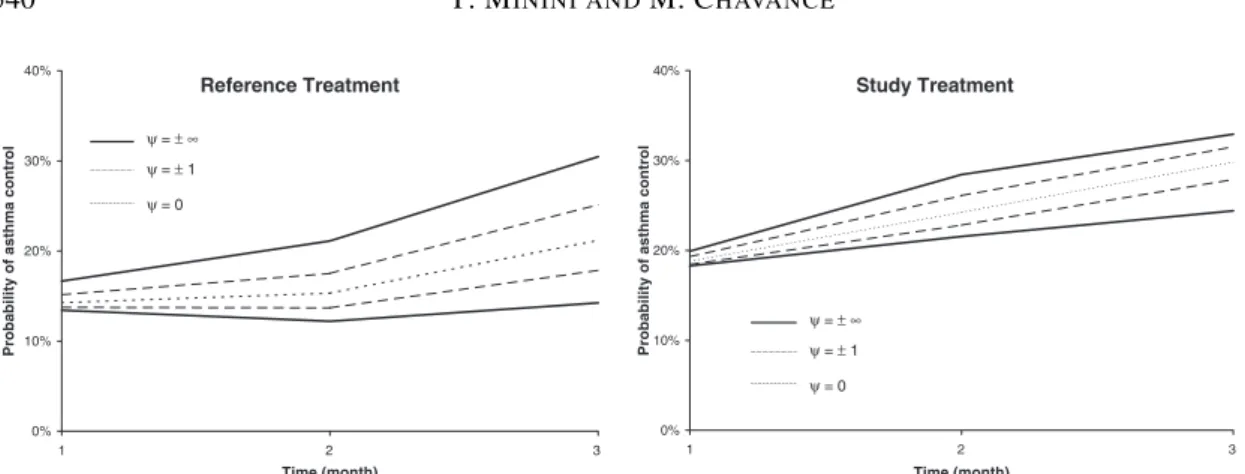
The aim of the study was to compare the mean evolution of the rate of asthma control between the two groups. This analysis included adjustments for sex and smoking status (smoker versus non-smoker). After estimation of the model as described in Section 3.2, multiple completed data sets were generated using the method described in Section 4. Each completed dataset was then analysed via a marginal model,
Reference Treatment 0% 10% 20% 30% 40% 1 2 3 Time (month)
Probability of asthma control
ψ = ±∞ ψ = ± 1 ψ = 0 Study Treatment 0% 10% 20% 30% 40% 1 2 3 Time (month)
Probability of asthma control
ψ = ±∞ ψ = ± 1
ψ = 0
Fig. 1. Estimation of monthly probability of asthma control in each treatment group, according to different values ofψ.
estimated by generalized estimated equations (see for example Xie and Paik, 1997). This marginal model could be written as
logitPYj =1|X=x
=µj+β1x1+β2x2+β3x3 (9) wherex1,x2andx3represent the treatment, sex and smoking status indicators respectively.
Thus, the effect of time was modelled qualitatively and the effect of treatment was assumed to be the same at each time of measurement. This was justified by the absence of significant treatment by time interaction. Finally, an unstructured matrix was used for the modelling of the within-subject correlations. For a better interpretation of the results of the sensitivity analysis, a preliminary approach is to estimate the probabilitiesPYj =1|X=x
, i.e. the marginal probabilities of asthma control at each month, within each treatment group, after adjustment for covariates. These probabilities are estimated for different values ofψand are displayed in Figure 1. As missing data were more frequent in the reference group, the effect of ψ was more important in this group than in the study treatment group, especially so for the third month. Finally, values−∞and+∞forψ, corresponding to the worst and best case respectively, delimit the range of all possible values for the estimated probabilities of asthma control.
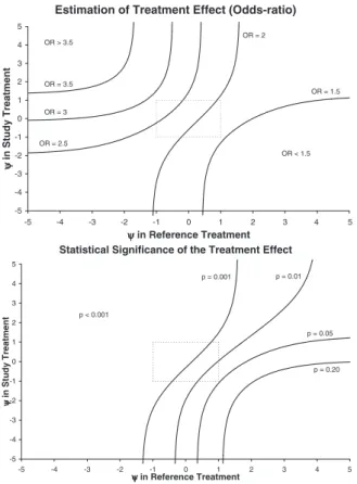
The results of this sensitivity analysis are presented in Figure 2. In the upper part of these graphs, each curve joins combinations ofψin both treatment groups for which the same estimate of the treatment effect (in terms of the odds-ratio between treatment groups) is obtained. In the lower part, couples ofψ with the same level of statistical significance are displayed. Inside the dotted box are reasonable values forψin both treatment groups, i.e.ψwithin±1. Outside of this box are more extreme values.
Assuming that missing data were ignorable (ψ=0) in both groups, a better asthma control was observed in the study treatment group, with an odds-ratio of 2.15 (p<0.001). In the range of values of ψwithin±1 in both groups, the treatment effect remained relatively stable, and a significant difference was still observed. The interval of ignorance was [1.56, 2.84]. Its associated 95% interval of uncertainty was [1.02, 4.37], which was entirely above 1.
Only assumptions outside the range of plausible values could raise a non-significant result, in particular, a strong nonignorable mechanism of opposed sign in the two groups, greatly disfavouring the treatment group. For example, the best case/worst case analysis, which corresponds toψ = −∞ in the treatment group and ψ = +∞ in the reference group, led to near equality between the two groups (OR=1.00) but did not reverse the conclusion of the study. It should be recalled that in this study, both groups received an active treatment, registered for asthma. Their safety profiles were comparable. Therefore, there seems to be no reason for assuming such a dramatic difference between their missing data processes.
Estimation of Treatment Effect (Odds-ratio) -5 -4 -3 -2 -1 0 1 2 3 4 5 -5 -4 -3 -2 -1 0 1 2 3 4 5 ψ ψ ψ ψ in Reference Treatment ψψψψ in Study Treatment OR = 1.5 OR = 2 OR = 2.5 OR = 3 OR = 3.5 OR < 1.5 OR > 3.5
Statistical Significance of the Treatment Effect
-5 -4 -3 -2 -1 0 1 2 3 4 5 -5 -4 -3 -2 -1 0 1 2 3 4 5 ψ ψ ψ ψ in Reference Treatment ψψψψ in Study Treatment p < 0.001 p = 0.001 p = 0.01 p = 0.05 p = 0.20
Fig. 2. Results of the sensitivity analysis: contour plot of the estimation of the treatment effect and statistical significance, for different values ofψin each treatment group.
In conclusion, the sensitivity analysis showed that the superiority of the study treatment was robust to slight to moderate departure from theignorabilityassumption. In this study, missing data should therefore not be considered to be a serious source of concern.
6. DISCUSSION
The fundamental impossibility to perform any valid inference without strong and untestable assump-tions justifies the choice of a sensitivity analysis: inferences under a range of plausible or extreme assumptions rather than a single inference. However, unless the treatment effect is very strong or the rate of missing data very low, it seems obvious that the most extreme assumptions will at least invalidate the statistical significance, and sometimes reverse the conclusion of a study (see examples provided by Rotnitzkyet al.1998, 2001; Scharfsteinet al.1999; Hollis 2002; Birminghamet al.2003). Our opinion is that one should not expect a conclusion to resist all assumptions about missing data, but only to remain stable under mild or moderate assumptions. In the example described in this paper, values ofψwithin
±1 could be considered as a reasonable compromise between the risk of neglecting plausible assumptions and that of considering unrealistic assumptions. In this case, the use of intervals of ignorance and intervals of uncertainty is valuable.
The log–linear model introduced in Section 2 may be debatable in some contexts, for example when the number of measurements is variable. However, in clinical trials the number of planned observations
is usually fixed, even if the number of responses actually observed may be variable across subjects due to missing data. The conditional character of this model also downplays its applicability, and a marginal model is often preferred for the analysis. But that does not preclude its usefulness for the imputation of the missing data. Indeed, in a marginal framework, the conditional distribution of missing data, given the observed data and the missing data structure, is often very complex. This conditional distribution is fundamental for imputation. On the other hand, in the log–linear model, this conditional distribution is easily derived.
Completing the data under various nonignorable assumptions, and then analysing them using a possibly different model, is in the spirit of multiple imputation (Schafer, 1999). It raises the classical issue of the difference between the imputer’s model and the analyst’s model (Rubin, 1996; Schafer, 1997). However, in this context, the imputer and the analyst would generally be the same person. Thus, the assumptions made for completing and analysing the data (concerning the time-dependance, within-subject correlations, effect of covariates) should be similar in the log–linear model and the marginal model.
An alternative to multiple imputation would be to perform a weighted analysis using the estimated probabilities P[M|X,Y], for example weighted GEE (Robins et al., 1995). However, note that some widely used procedures such as SAS proc genmod allow the introduction of known weights, but do not take into account their imprecision when they are estimated, and thus underestimate the variance of the weighted estimation.
Imputations are generated under anonignorablemodel and inferences performed are valid under the assumed mechanism for missing data. One may legitimately wonder to what extent the conclusions of the analysis depend on the model assumptions. Clearly, the adequacy of the model to the observations has to be checked using diagnostic tools, but one cannot expect the examination of the available residuals or influence measures to shed light on the choice ofψ. In this modelling, several assumptions were set. First of all, the association between any pair of responses was assumed not to depend on the missing data pattern. Secondly, it was assumed that conditionally onYj, the missingness ofYj was independent of all
otherYk. Finally, it was assumed thatψwas constant over time. These assumptions cannot be checked,
and thus have the potential to raise doubts about the robustness of the method.
The method for conducting a sensitivity analysis proposed in this paper can be extended by removing one or all of these assumptions, but at the cost of a higher-dimensional analysis, and a loss of simplicity and interpretability. Conversely, a simple model with a parameterψ fixed in each treatment group will generally cover all the situations of practical interest. If the conclusion of the study is robust over a range of values forψin each group, one can expect it would also resist a more complex model.
The flexibility of the log–linear model allows us to consider alternative assumptions. For instance, in some contexts it may be more plausible for missingness to depend on other variables than on the variable subjected to missingness itself. In this case, from model (1), one would assume thatψj j =0 and derive a
different model. Note that this would not necessarily lead to an ignorable model, since missingness could be assumed to depend on the previous response, which is also possibly missing.
Other possible extensions may include the handling of the cause of missing data. In clinical trials, these reasons are often investigated. In some cases, the missingness is likely to be unrelated to the unobserved response, for example the refusal to continue for personal convenience or the technical impossibility to perform the measure. In other cases, one would not assume that there exists an unobserved value behind the missing values, especially when dropout corresponds to the death of the subject. In these cases, a simple extension of the proposed method would consist in imputing only missing values considered as potentially related to the existing unobserved response.
A drawback of this method is the weight of calculations, which exponentially increases with the number of measurements by subject(n)and the number of explanatory variables(p). In particular, the EM algorithm involves 22n+psufficient statistics, so that with our computer (a Pentium III 1.4 GHz), this method could not be applied withn10.
ACKNOWLEDGEMENTS
The authors are grateful to Florence Casset-Semanaz for her constant support in this research work. We are also grateful to two anonymous reviewers for their insightful comments that greatly contributed to improving the quality of this paper.
Minini’s research was partially supported by the French Association Nationale de la Recherche Technique, Convention CIFRE 707/2000.
REFERENCES
BAKER, S. G., ROSENBERGER, W. F.ANDDERSIMONIAN, R. (1992). Closed-form estimates for missing counts in two-way contengency tables.Statistics in Medicine11, 643–657.
BIRMINGHAM, J., ROTNITZKY, A. AND FITZMAURICE, G. M. (2003). Pattern-mixture and selection models for analysing longitudinal data with monotone missing patterns.Journal of the Royal Statistical Society, Series B65, 275–297.
BISHOP, Y. M. M., FIENBERG, S. E.ANDHOLLAND, P. W. (1975).Discrete Multivariate Analysis: Theory and Practice. Cambridge, MA: MIT Press.
COMMITTEE FOR PROPRIETARY MEDICINAL PRODUCTS (2001). Points to consider on missing data, CPMP/EWP/1776/99.European Agency for the Evaluation of Medicinal Products, London.
COPAS, J. B.AND LI, H. G. (1997). Inference for non-random samples (with discussion).Journal of the Royal Statistical Society, Series B59, 55–95.
DEMPSTER, A. P., LAIRD, N. M.ANDRUBIN, D. B. (1977). Maximum likelihood estimation from incomplete data via the EM algorithm (with discussion).Journal of the Royal Statistical Society, Series B39, 1–38.
DIGGLE, P. J.ANDKENWARD, M. G. (1994). Informative drop-out in longitudinal data analysis (with discussion). Applied Statistics43, 49–93.
DIGGLE, P. J., HEAGERTY, P., LIANG, K. Y.ANDZEGER, S. L. (2002).Analysis of Longitudinal Data, 2nd edition. Oxford: Oxford University Press.
FITZMAURICE, G. M.ANDLAIRD, N. M. (2000). Generalized linear mixture models for handling nonignorable dropouts in longitudinal studies.Biostatistics1, 141–156.
FOLLMANN, DANDWU, M. (1995). An approximate generalized linear model with random effects for informative missing data.Biometrics51, 151–168.
GROSCLAUDE, M. AND DESFOUGERES, J. L. (2003). Fluticasone/Salmeterol (FP/S) est plus efficace que l’association beclomethasone-montelukast (BDP-M).Revue de Maladies Respiratoires20, 1S74–1S74.
HOLLIS, S. (2002). A graphical sensitivity analysis for clinical trials with non-ignorable missing binary outcome. Statistics in Medicine21, 3823–3834.
IBRAHIM, J., CHEN, M. H.ANDLIPSITZ, S. R. (2001). Missing responses in generalized linear mixed models when the missing data mechanism is nonignorable.Biometrika88, 551–564.
JAMSHIDIAN, M.ANDJENNRICH, R. I. (2000). Standard errors for EM estimation.Journal of the Royal Statistical Society, Series B62, 257–270.
KENWARD, M. G., GOETGHEBEUR, J. T. ANDMOLENBERGHS, G. (2001). Sensitivity analysis for incomplete categorical data.Statistical Modelling1, 31–48.
LIPSITZ, S. R,, MOLENBERGHS, G., FITZMAURICE, G. M. AND IBRAHIM, J. (2000). GEE with Gaussian estimation of the correlations when data are incomplete.Biometrics56, 528–536.
LITTLE, R. J. A. (1994). Discussion to Diggle and Kenward: Informative drop-out in longitudinal data analysis. Applied Statistics43, 78.
LITTLE, R. J. A. (1994). A class of pattern-mixture models for normal incomplete data.Biometrika81, 471–483. LITTLE, R. J. A. (1995). Modelling the drop-out mechanism in repeated measures studies.Journal of the American
Statistical Association90, 1112–1121.
LITTLE, R. J. A.ANDRUBIN, D. B. (1987).Statistical Analysis with Missing Data. New York: Wiley.
MOLENBERGHS, G., KENWARD, M. G. AND GOETGHEBEUR, E. (2001). Sensitivity analysis for incomplete contingency tables: the Slovenian plebiscite case.Applied Statistics50, 15–29.
PAIK, M. C. (1997). The generalized estimating equation approach when data are not missing completely at random. Journal of the American Statistical Association92, 1320–1329.
ROBINS, J. M., ROTNITZKY, A. AND ZHAO, L. P. (1995). Analysis of semi-parametric regression models for repeated outcomes in the presence of missing data.Journal of the American Statistical Association90, 106– 121.
ROTNITZKY, A., ROBINS, J. M. ANDSCHARFSTEIN, D. (1998). Semiparametric regression for repeated outcomes with nonignorable nonresponse.Journal of the American Statistical Association93, 1321–1339.
ROTNITZKY, A., SCHARFSTEIN, D., SU, T. L.ANDROBINS, J. M. (2001). Methods for conducting sensitivity analysis of trials with potentially nonignorable competing causes of censoring.Biometrics57, 103–113.
RUBIN, D. B. (1987).Multiple Imputations for Nonresponse in Surveys. New York: Wiley.
RUBIN, D. B. (1994). Discussion to Diggle and Kenward: Informative drop-out in longitudinal data analysis.Applied Statistics43, 80–82.
RUBIN, D. B. (1996). Multiple imputation after 18+ years.Journal of the American Statistical Association91, 473– 489.
SAS INSTITUTEINC. (1999). SAS/STAT User’s guide, Version 8, Cary, NC.
SCHAFER, J. L. (1997).Analysis of Incomplete Multivariate Data. New York: Chapman and Hall. SCHAFER, J. L. (1999). Multiple imputation: a primer.Statistical Methods in Medical Research8, 3–15.
SCHARFSTEIN, D., ROTNITZKY, A. AND ROBINS, J. M. (1999). Adjusting for nonignorable dropout using semiparametric nonresponse models (with discussion).Journal of the American Statistical Association94, 1096– 1146.
SKINNER, C. J. (1997). Discussion to Copas and Li: Inference for non-random samples. Journal of the Royal Statistical Society, Series B59, 55–95.
UNNEBRINK, K.ANDWINDELER, J. (1999). Sensitivity analysis by worst and best case assessment: is it really sensitive?.Drug Information Journal33, 835–839.
VANSTEELANDT, S., GOETGHEBEUR, E., KENWARD, M. G. ANDMOLENBERGHS, G. (2000). Ignorance and uncertainty regions as inferential tool in a sensitivity analysis.Technical Report 2000/2,Centrum voor Statistiek. Ghent University.
VANSTEELANDT, S. ANDGOETGHEBEUR, E. (2001). Analyzing the sensitivity of generalized linear models to incomplete outcomes via the IDE algorithm.Journal of Computational and Graphical Statistics10, 656–672. VERBEKE, G.ANDMOLENBERGHS, G. (2000).Linear Mixed Models for Longitudinal Data. New York: Springer. XIE, F.ANDPAIK, M. C. (1997). Multiple imputation methods for the missing covariates in generalized estimating
equations.Biometrics53, 1538–1546.
[Received 16 June 2003; first revision 28 October 2003; second revision 5 February 2004; accepted for publication 12 February 2004]