ESTIMATING THE NUMBER OF SHARED SPECIES IN TWO COMMUNITIES

ESTIMATING THE NUMBER OF SHARED SPECIES IN TWO COMMUNITIES

Anne Chao∗, Wen-Han Hwang∗, Y-C Chen∗ and C-Y Kuo

∗_{National Tsing Hua University and Wild Bird Society of Hsin-Chu}

Abstract: In statistical ecology, the number of shared species is a standard measure of similarity between two communities. Assume that a multinomial sample is drawn from each of the two target communities. Each observation (individual) in the sample is classified to species identity, and the frequency for each observed species is recorded. This paper uses the concept of sample coverage to estimate the number of species in common to the two communities (the number of shared species). The result generalizes Chao and Lee (1992) to a two-community situation. Simulation results are reported to examine the performance of the proposed estimators. Bird census data collected from April 1994 to March 1995 in Ke-Yar and Chung-Kang estuaries in Taiwan are used to illustrate the estimation procedure.

Key words and phrases: Coefficient of covariation, coefficient of variation, com-munity similarity, heterogeneity, multinomial, overlap, sample coverage, shared species.

1. Introduction

Estimating the number of species in a community is a classical problem in ecology, biogeography, and conservation biology, and parallel problems arise in many other disciplines. This research topic has been extensively discussed in the literature; see Bunge and Fitzpatrick (1993), Seber (1982, 1986, 1992) for a review of the historical and theoretical development. In a subsequent paper, Bunge, Fitzpatrick and Handley (1995) also compared three principal frequentist procedures using simulation results. Ecologists and other biologists have long recognized that there are undiscovered species in almost every survey or species inventory.

Very often, comparison of two communities is required in ecological applica-tions and environmental policy decisions. The two communities could be candi-date sites for conservation or restoration, or areas at different latitudes or eleva-tion above sea level (Colwell (1973), Colwell and Coddington (1994), Feinsinger (1976), Karr, Robinson, Blanke and Bierregaard (1990)), or could represent the same area at two different times, e.g., before and after pollution (Grassle and Smith (1976)). We were motivated by the bird data collected in two estuaries in Taiwan. These two river estuaries (Ke-Yar River and Chung-Kang River)

are only 20 kilometers apart and both have been heavily polluted. Bird data were collected every Sunday morning from April 1994 to March 1995 in these two areas. These two areas share many species because of similar environments for both resident and migratory birds. The local wild bird society is especially interested in knowing whether there were species present in both estuaries but not observed in both, during this year-long survey.

A common approach to comparing two communities is to measure the extent of “similarity” (using an overlap index) or “dissimilarity”. For example, Gower (1985) listed 15 different overlap measures based on various justifications; see also Pielou (1975, 1976) and Ludwig and Reynolds (1988) for details. Grassle and Smith (1976) proposed a new measure of similarity based on the expected number of species shared between sub-samples of larger collections for two sites. Colwell and Coddington (1994) suggested the use of a dissimilarity measure called “com-plementarity”. All these measures are functions of the number of species shared by two samples. Hence an estimator of the shared species plays an important role in comparing two communities. Surprisingly, ecologists have generally used the observed number of shared species as the real number of shared species. To our knowledge, there has been little discussion in the literature regarding the es-timation of unobserved shared species. It seems worthwhile to explore eses-timation procedures for this topic.

Section 2 briefly reviews the sample coverage approach for the one-community case, since some background is needed for extension. Section 3 presents the model for the two-community case and the procedure to estimate the number of shared species. Simulation results are reported in Section 4 to investigate the performance of the proposed estimators. The bird data collected in the two estuaries in Taiwan, as described above, are used in Section 5 to il-lustrate the estimation procedure. Details on the data (Chen, Hwang, Chao and Kuo (1995)) appeared in Chinese in the Journal of Chinese Statistical Associa-tion. A program EstimateS(Colwell (1997)) which calculates various estimators of species richness including the sample coverage approach is readily available from the website http://viceroy.eeb.uconn.edu/estimates.

2. Review of Estimation for One Community

This section reviews the sample coverage approach to estimating the number of species for one community. Assume that there areS species in the community and they are indexed by 1, . . . , S. Denote the probabilities of species discovery by = (π₁, . . . , π_S) where S_i=1π_i = 1. A random sample of size m is taken with replacement from the community and each individual is classified correctly to species identity. Let X_i be the number of individuals of the ith species ob-served in the sample. ThusS_i=1X_i =m. Here we remark that the summation

is just over all the observed species because any unobserved species (X_i = 0) would not contribute to the sum. The same remark applies to similar summa-tions throughout this paper. The frequencies (X₁, . . . , X_S) are multinomially distributed.

The basic idea is that, whereas it is difficult to estimate the number of species when probabilities of species discovery are heterogeneous, the sample coverage can nonetheless be well-estimated in such a case. (The sample coverage is defined below.) Therefore, we first estimate the sample coverage and then use it to estimate the number of species. Refer to Chao and Lee (1992), Chao, Ma and Yang (1993) for details. The following notation generally follows that used in Chao and Lee (1992) and Colwell (1997).

In the sample coverage approach, the frequencies (X₁, . . . , X_S) are first clas-sified into “frequency counts” (f₁, . . . , f_m), where m is the sample size and f_k

denotes the number of species that were observed exactlyktimes in the sample, that is, f_k = S_j=1I[X_j = k], where I[.] is the usual indicator function. Note that the zero-frequency f₀ is unobservable and the problem is then reduced to estimating the expected value off₀. It is intuitively clear that species that occur many times would be discovered in any sample anyway, so they carry almost no information regarding the number of unobserved species. Only those species with small discovery probabilities would be either unobserved or observed once, twice,. . . or only a few times. Therefore, the lower-order frequency counts carry nearly all available information about zero-frequency. We base the estimate of unobserved species on (f₁, . . . , f₁₀), then complete the estimate by adding on the number of species each represented by more than 10 individuals. The cut-off number 10 has been selected based on empirical experiences, see Chao, Ma and Yang (1993).

Conceptually, the foregoing arguments lead to separating the observed species into two groups: abundant and rare. Only the latter group is used to estimate the number of unobserved species. That is, we consider only a sub-community by temporarily ignoring the abundant species. Let the total number of abundant species in the sample be S_abun = m_k=11f_k =S_i=1I[X_i >10] and the number of observed rare species be S_rare=10_k=1f_k=S_i=1I[0< X_i ≤10]. Hence there are N = S−S_abun species in the sub-community, counting unob-served as well as obunob-served rare species. Since we can permute the species ordering so that all the abundant species are the last ones, the data restricted to the sub-community become (X₁, . . . , X_N). The sample size reduces ton =10_k=1kf_k =

m−S_i=1X_iI[X_i > 10]. Theoretically it can be verified that the frequencies (X₁, . . . , X_N) are also distributed as a multinomial distribution with cell proba-bility P = (p₁, . . . , p_n) where p_i = π_i/{1−S_j=1π_jI[X_j > 10]}. Therefore, the data restricted to the sub-community also have a multinomial model structure.

It is statistically impossible, but fortunately also unnecessary, to identify each single cell probability inP= (p₁, . . . , p_N). We assume that the information on the species discovery probabilities is concentrated in a non-negative measure called “coefficient of variation” (CV). The CV for the sub-community is defined as γ = [N−1N_i=1(p_i −p)2]1/2/p where p = N_i=1p_i/N = 1/N. The value of CV characterizes the degree of heterogeneity among the p_i’s (or in ecological terminology, the degree of numerical dominance in the relative abundance distri-bution). The CV vanishes if and only if the sub-community is homogeneous (i.e., all p_i’s are equal). The larger the CV, the greater the degree of heterogeneity among species in probability of discovery. The most difficult part in this estima-tion procedure lies with the estimaestima-tion of CV, especially when CV is relatively large and data are sparse. The whole community with both abundant and rare species would typically have a large value of CV. Therefore, another important reason for considering only rare species is that the CV for the restricted sub-community is substantially lower than that of the whole sub-community. Hence we can obtain a more sensitive and reliable estimate of CV for the sub-community.

The sample coverage is mathematically defined as

C =

N

i=1

p_iI[X_i >0].

In effect, the sample coverage represents the fraction of actual total (rare) species that is discovered in the sample. We can interpret 1−C as the conditional (on data) probability of discovering a new species if an additional observation (indi-vidual) were to be taken. A well-known estimator, originally proposed by Turing (see Good (1953)), for this conditional probability is the proportion of singletons in the sample (i.e., f₁/10_k=1kf_k). This can be intuitively understood because a new species must be a singleton in the enlarged sample including the additional individual. The sample coverage estimate for the sub-community thus becomes

ˆ

C= 1−f₁/10_k=1kf_k. This estimator performs well even in heterogeneous cases, e.g., Esty (1986).

It follows from the definition of the sample coverage that if p₁ =p₂ =· · ·=

p_n = 1/N, then C = S_rare/N, where S_rare is the number of rare species in the sample. Hence a valid estimator in the homogeneous cases for the sub-community is

ˆ

N0 =S_rare/C.ˆ

Consequently, the proposed estimator for the whole community in the homoge-neous case is

ˆ

If heterogeneity (species dominance) is present, we attempt to account for the heterogeneity by adjusting S_rare/Cˆ based on an estimate of the parameter CV. The proposed estimator of N is

ˆ N = Srare ˆ C + f₁ ˆ Cˆγ 2_,

where ˆγ2 = max{(S_rare/Cˆ)10_i=1i(i−1)f_i/[n(n−1)]−1,0}denotes the estimator of squared CV (Chao and Lee (1992)). For a homogeneous case, the last term is not needed because the CV is 0. Thus the term that is proportional to the magnitude of heterogeneity represents the undercount if we adopt an estimator without considering heterogeneity in a heterogeneous community. Adding in the number of abundant species, we obtain an estimate for the whole community as

ˆ S =S_abun+Srare ˆ C + f₁ ˆ Cˆγ 2_{. (2.2)}

An analytic approximate standard error of ˆS0 and ˆSis provided in Chao and Lee (1992).

3. Models and Estimators for Two Communities

We now extend our approach to the case of two communities. Assume that there areS₁species in community I and there areS₂species in community II. The probabilities of species discovery in community I and II are denoted respectively by = (π₁, . . . , π_S1) and ∗ = (π₁∗, . . . , π∗_S2) where π_i >0,π∗_i >0,S_i=11 π_i = 1 and S_i=12 π_i∗ = 1. Let the number of shared species be S₁₂, the parameter of interest.

Two random samples (sample I and sample II) of sizesm₁and m₂ are taken respectively from community I and II. Assume that S_1(obs) and S_2(obs) distinct species are actually observed in sample I and II respectively, andS_12(obs)distinct shared species are observed. As in the one-community case, we first separate our observed shared species into two groups. One group (“abundant shared species”) includes species with at least one of the frequencies greater than 10, and the other group (“rare shared species”) includes species with both frequencies less than or equal to 10. We rely exclusively on this group of “rare shared species” to estimate the number of unobserved shared species, then add in the number of abundant shared species to the resulting estimate. Let the number of abundant shared species beS_12(abun). By temporarily setting aside these abundant shared species, we perform inference on the restricted two sub-communities.

As in the one-community case, the data confined to the sub-communities have the same probability structures as in the original communities. There are

N₁ =S₁−S_12(abun) species in sub-community I with probability of species dis-coveryP= (p₁, . . . , p_N1) wherep_i>0 for alliandN_i=11 p_i = 1. The relationship between = (π₁, . . . , π_S1) and P = (p₁, . . . , p_N1) can be easily formulated, as indicated in the previous section. Similarly, we haveN₂=S₂−S_12(abun) species in the sub-community II with species discovery probabilities P∗= (p∗₁, . . . , p∗_N2),

p∗_i > 0 for all i and N_i=12 p∗_i = 1. In the two sub-communities, the number of shared species becomesN₁₂=S₁₂−S_12(abun). Without loss of generality, assume that the firstN₁₂species in Pand P∗ are these shared species.

Denote the observed frequencies in the two sub-communities by (X₁, . . . , X_N1) and (Y₁, . . . , Y_N2) respectively. The reduced samples sizes aren₁=N1

i=1Xi

and n₂ = N2

i=1Yi. In the two sub-communities, the number of distinct (rare)

shared species in the samples becomes S_12(rare) =S_12(obs)−S_12(abun). For nota-tional simplicity, we denote S_12(rare) by M₁₂ in the following derivations. That is, S_12(rare) ≡ M₁₂ = N_i=112I[0 < X_i ≤ 10,0 < Y_i ≤ 10]. Again, we can as-sume that these observed shared species are the first M₁₂ species in the actual

N₁₂ shared species. For index i= M₁₂+ 1, M₁₂+ 2, . . . , N₁₂, we have X_i = 0,

Y_i = 0; or Y_i = 0, X_i = 0; or X_i = Y_i = 0. In the first two situations, the ith species appears in one of the two samples as a unique species, but it is actually an unobserved shared species because it was missed in the other sample.

The extension to the estimation of the number of shared species in two com-munities is not directly obvious. In addition to a heterogeneity measure for each community, we also need a parameter to specify the “dependence” of the two sets of species probabilities P and P∗. Therefore, three parameters are needed. It would be conceptually simpler if we could adopt the use of two heterogeneity measures and one dependence measure in the inference. However, this approach results in some non-estimable quantities. We thus need to introduce one ad-ditional set of probabilities Q = (Q₁, . . . , Q_N12), for the shared species where

Q_i = p_ip∗_i. The three measures (two heterogeneity parameters and one depen-dence parameter) are then reparameterized into the following three parameters called “coefficient of covariation” (CCV). We define them in the following two types of models:

• Fixed-effects model:

Assume that the average of the shared species probabilities (p₁, . . . , p_N12) in sub-community I is p; and the average for the shared species probabilities (p∗₁, . . . , p∗_N12) in sub-community II is p∗. Let Q = N_i=112Q_i/N₁₂. Define the following coefficients of covariation (CCV):

CCV ofPand Q: Γ₁=N

−1

12 Ni=112(pi−p)(Q_i−Q)

CCV ofP∗ and Q: Γ₂=N −1 12 Ni=112(p∗i −p∗)(Qi−Q) p∗Q , CCV ofP,P∗ andQ: Γ₁₂=N −1 12 Ni=112(pi−p)(p∗i −p∗)(Qi−Q) p∗Q . • Random-effects model:

Assume that (p_i, p∗_i), i = 1, . . . , N₁₂, are a random sample from a two di-mensional distribution F(p, p∗) with marginal distributions F₁(p) and F₂(p∗). Letp₀= pdF₁(p),p∗₀=p∗dF₂(p∗) and Q₀ = pp∗dF(p, p∗). Define

CCV of Pand Q: Γ₁= (p−p₀)(pp∗−Q₀)dF(p, p∗) p₀Q₀ , CCV ofP∗ and Q: Γ₂= (p∗−p∗₀)(pp∗−Q₀)dF(p, p∗) p∗₀Q₀ , CCV ofP,P∗ and Q: .Γ₁₂= (p−p₀)(p∗−p∗₀)(pp∗−Q₀)dF(p, p∗) p₀p∗₀Q₀ .

In a random-effects model, the two sets of probabilities P and P∗ are called independent if F(p, p∗) =F₁(p)F₂(p∗), which implies that h(p)g(p∗)dF(p, p∗) =

h(p)dF₁(p)×g(p∗)dF₂(p∗) for any functionshandg. In a fixed-effects model, the independence assumption means thatN₁₂−1N12

i=1h(pi)g(p∗i) = [N12−1Ni=112h(pi)] ×[N₁₂−1N_i=112g(p∗_i)]. As a special case, we haveN₁₂−1_i=1N12pα_i(p∗_i)β= [N₁₂−1N_i=112pa_i]

×[N₁₂−1N_i=112(p∗_i)β] for any positive integers α and β.

In the following, we use a fixed-effects model approach to obtain the proposed estimators. The random-effects model will produce exactly the same estimators. First, the intuitive meaning of the parameters CCV can be understood by con-sidering the following special cases.

(1) If both sets of species probabilities P and P∗ are homogeneous, then they are independent. We can readily see that Γ₁= Γ₂= Γ₁₂= 0.

(2) If p₁p∗₁ =p₂p∗₂ = · · · = p_N12p∗_N12 (i.e., the set of probabilities Q is homoge-neous), then it follows from the definition that Γ₁ = Γ₂ = Γ₁₂ = 0. Note that in this case, the two sets of probabilities P and P∗ are not necessarily independent.

(3) When community I is heterogeneous but community II is homogeneous, it is clear that the two sets of probabilities are independent. The CCVs in this case are Γ₂ = Γ₁₂ = 0 and Γ₁ =γ₁2 = [N₁₂−1N_i=112(p_i−p)2]/p2, which is the squared CV of the shared species in community I. Similarly, if community I is homogeneous but community II is heterogeneous, then Γ₁ = Γ₁₂ = 0 and Γ₂ =γ2₂ = [N₁₂−1_i=1N12(p∗_i −p∗)2]/p∗2, the squared CV of the shared species in community II.

(4) If both communities are heterogeneous, but the two sets of probabilities are independent, simple expansion leads to Γ₁ = γ₁2, Γ₂ = γ₂2 and Γ₁₂ =γ₁2γ₂2. Hence in the special case of independence, only the two CVs need to be identified in the analysis.

Although in the above special cases, all CCVs appear to be nonnegative, they could be negative in other situations. In general, the CCVs can be expressed as:

Γ₁=N12σ21 σ₁₀σ₁₁ −1, Γ2 = N₁₂σ₁₂ σ₀₁σ₁₁ −1, (3.1a) Γ₁₂= N 2 12σ22 σ₁₀σ₀₁σ₁₁ − N₁₂σ₁₁ σ₀₁σ₁₀ −Γ1−Γ2, (3.1b) whereσ_αβ =N_i=112pα_i(p∗_i)β.

We now define the sample coverage for the two sub-communities as follows:

C₁₂= _N12 i=1pip∗iI[Xi >0, Yi >0] _N12 i=1pip∗i . (3.2)

Thus the sample coverage represents the fraction of product probabilities associ-ated with the shared species that were discovered in both samples. Note that

I[X_i >0, Y_i >0] = 1−I[X_i = 0]−I[Y_i = 0] +I[X_i = 0, Y_i = 0]. Then E(C₁₂) = 1− _N12 i=1pip∗i[(1−pi)n1 _{+ (1−p}∗ i)n2 −(1−pi)n1_(1−p∗ i)n2] _N12 i=1pip∗i . (3.3) ≈1− _N12 i=1pip∗i[(1−pi)n1−1+ (1−p∗)n2−1−(1−pi)n1−1(1−p∗i)n2−1] N12 i=1pip∗i .

The last approximation is valid if the sample sizes n₁ and n₂ are large enough. Based on the moments of the multinomial distribution, we can verify that

E M12 i=1 X_iY_i =n₁n₂ N12 i=1 p_ip∗_i, (3.4) E M12 i=1 X_iI[Y_i = 1] =n₁n₂ N12 i=1 p_ip∗_i(1−p∗_i)n2−1, E M12 i=1 Y_iI[X_i = 1] =n₁n₂ N12 i=1 p_ip∗_i(1−p_i)n1−1, E M12 i=1 I[X_i =Y_i = 1] =n₁n₂ N12 i=1 p_ip∗_i(1−p_i)n1−1_(1−p∗ i)n2−1.

Hence an estimator of the sample coverage can be seen to be ˆ C₁₂= 1− _M12 i=1{YiI[X_i = 1] +X_iI[Y_i= 1]−I[X_i =Y_i = 1]} _M12 i=1 XiYi (3.5)

In obtaining (3.5), we use the approximation that the expectation of a ratio is approximately the ratio of the expectations. The discrepancies here are negligible when sample coverage is not too low (say, not less than 70%). Unless there are many shared species that are abundant in one community but rare in the other, the sample coverage estimator (3.5) performs well, as we will see in the simulation section. As in the one-community case, the number of singletons in each sample plays an important role in the estimation of sample coverage. It follows from the definition in (3.2) that if the set of probabilities Q is homogeneous, that is, p₁p∗₁ = p₂p∗₂ = · · · = p_N12p∗_N12, then C₁₂ = M₁₂/N₁₂. Therefore, a natural estimator ofN₁₂ when all product probabilities are equal is

ˆ

N₁₂0 =M₁₂/Cˆ₁₂=S_12(rare)/Cˆ₁₂. (3.6) Also notice that

E(M₁₂) = N12 i=1 = N12 i=1 [1−(1−p_i)n1][1−(1−p∗_i)n2]. (3.7)

This implies that E(M₁₂)/E(C₁₂) = N₁₂ if Q is homogeneous. However, the identity is no longer valid if Q is heterogeneous. To evaluate the discrepancy between E(M₁₂)/E(C₁₂) and N₁₂ in such cases, we need more notation. Let

f₁₊ =M_i=112I[X_i = 1, Y_i ≥1] be the number of shared species which are single-tons in sample I; f₊₁ =M_i=112I[X_i ≥1, Y_i = 1] be the number of shared species which are singletons in sample II; f₁₁ =M_i=112I[X_i = 1, Y_i ≥1] be the number of shared species which are singletons in both samples. A simple expansion of

E(M₁₂)/E(C₁₂) results in the following:

M(M₁₂)

E(C₁₂) =N12− 1

E(C₁₂)[E(f1+)Γ1+E(f+1)Γ2+E(f11)Γ12] +R, (3.8)

where R is a remainder term. The magnitude of R depends on the two sets of P and P∗. We provide the following justifications of ignoring the remainder term.

(1) If both sets of species probabilities are homogeneous, it is easy to check that

R= 0.

(3) If community II is homogeneous and community I is heterogeneous, where (p₁, . . . , p_N1) is a random sample from a Dirichlet distribution, then we can show thatR/N₁₂converges to 0 asN₁₂grows large andn₁/N₁₂→c₁ >0. The above result is mainly based on Chen (1980). See Chen, Hwang, Chao and Kuo (1995) for details. Similar results hold if community I is homogeneous and community II is heterogeneous.

(4) Consider the following special (independent) heterogeneous case: If (p₁, . . . , p_N1) is a random sample from a Dirichlet distribution with parameter aand (p∗₁, . . . , p∗_N2) is also a random sample from a Dirichlet with parameter b, then R/N₁₂ tends to 0 as N₁₂ grows large enough, n₁/N₁₂ → c₁ > 0 and

n₂/N₁₂→c₂ >0.

If R can be ignored in the expansion of (3.8), then we can subsequently obtain estimators if the CCV parameters can be estimated. Note that

E M12 i=1 X_i =n₁ N12 i=1 p_i[1−(1−p∗_i)n2]≈n₁ N12 i=1 p_i, E M12 i=1 Y_i=n₂ N12 i=1 p∗_i[1−(1−p_i)n1_]≈n 2 N12 i=1 p∗_i, E M12 i=1 X_i(X_i−1)Y_i =n₁(n₁−1)n₂ N12 i=1 p2_ip∗_i, E M12 i=1 Y_i(Y_i−1)X_i =n₂(n₂−1)n₁ N12 i=1 (p∗_i)2p_i, E M12 i=1 X_i(X_i−1)Y_i(Y_i−1) =n₁(n₁−1)n₂(n₂−1) N12 i=1 p2_i(p∗_i)2.

Based on the above identities and the expressions (3.1a), (3.1b), (3.4), the CCV can be estimated as follows:

ˆ Γ₁= Nˆ 0 12n1T₂₁ (n₁−1)T₁₀T₁₁ −1, Γˆ2 = ˆ N₁₂0 n₂T₁₂ (n₂−1)T₀₁T₁₁ −1, (3.9a) ˆ Γ₁₂= n1n2( ˆN 0 12)2T22 (n₁−1)(n₂−1)T₁₀T₀₁T₁₁− ˆ N₁₂0T₁₁ T₀₁T₁₀ −Γˆ1−Γˆ2, (3.9b) where T₁₀= M12 i=1 X_i, T₀₁= M12 i=1 Y_i, T₁₁= M12 i=1 X_iY_i, T₂₁= M12 i=1 X_i(X_i−1)Y_i, T₁₂= M12 i=1 X_iY_i(Y_i−1), T₂₂= M12 i=1 X_i(X_i−1)Y_i(Y_i−1).

Using the concept of sample coverage and the estimates of the CCVs, we propose the following estimator of the number of shared species for the sub-communities:

ˆ N₁₂= M12 ˆ C₁₂ + 1 ˆ C₁₂[f1+ ˆ Γ₁+f₊₁Γˆ₂+f₁₁Γˆ₁₂], (3.10) where ˆC₁₂ is derived in (3.5). Adding the number of abundant shared species,

S_12(abun), to the resulting estimator, we have the following estimator for the whole communities when Qis homogeneous:

ˆ

S₁₂0 =S_12(abun)+ ˆN₁₂0 =S_12(abun)+S_12(rare)/Cˆ₁₂. (3.11a) If Q is heterogeneous (in which case the data should yield relatively large esti-mated CCVs), our estimator becomes

ˆ

S₁₂=S_12(abun)+ ˆN₁₂=S_12(abun)+S12(rare) ˆ C₁₂ + 1 ˆ C₁₂[f1+ ˆ Γ₁+f₊₁Γˆ₂+f₁₁Γˆ₁₂]. (3.11b) Note that (3.11a) and (3.11b) are natural extensions of (2.1) and (2.2).

An analytic variance estimator for the proposed estimators is still not avail-able. We suggest, instead, the use of a bootstrap procedure. First we divide the data into two parts: shared species {(X_i, Y_i), X_i >0, Y_i >0, i= 1, . . . , M12}

and unique species (one of the frequencies is 0). The bootstrap procedure is ap-plied only to the shared species part since the unique species have little effect on the resulting estimation (they change only the sample size, due to restriction to sub-communities, and thus affect the CCV estimates only slightly). Consider a “shared” population with ˆN₁₂shared species. There areM₁₂“observable” shared species with frequencies (X_i, Y_i), i= 1, . . . , M₁₂, and ˆN₁₂−M₁₂ “unobservable” shared species with frequencies (0, 0). The cell probability for each pair (X_i, Y_i) is 1/Nˆ₁₂. A random sample of size ˆN₁₂is drawn with replacement from this pop-ulation of paired values and a bootstrap replication {(X_i∗, Y_i∗), i = 1, . . . ,Nˆ₁₂}

can be generated. Then based on the replication and the observed unique species in the original sample, estimates ˆN₁₂∗ for the sub-communities and ˆS₁₂∗ for the whole communities are calculated. After B replications, we have B estimates

{_Sˆ∗1

12, . . . ,Sˆ12∗B} and the bootstrap variance estimator is the sample variance of

the resulting B estimates. The performance of this bootstrap standard error estimation will be examined in the following section.

4. Simulation Study

A simulation study was carried out to investigate the performance of the pro-posed estimator (3.11a) for the homogeneous case and the estimator (3.11b) for the heterogeneous case. We considered one homogeneous and four heterogeneous

communities with 200 species in each; the five sets of species discovery probabil-ities are given as follows. (The constant c in Cases II and IV is a normalizing constant such that the sum of species probabilities is equal to 1.)

Community I: π_i = 0.005, i= 1, . . . ,200. Community II:π_i =c/(i+ 10), i= 1, . . . ,200.

Community III: π_i = 0.01, i = 1−50; π_i = 0.005, i = 51−100; π_i = 0.003,

i= 101−150; π_i = 0.002, i= 151−200. Community IV:π_i =c/i,i= 1, . . . ,200.

Community V: (π₁, . . . , π₂₀₀) represents a random sample from a Dirichlet tribution with parameter 2, which is a multivariate generalization of a beta dis-tribution.

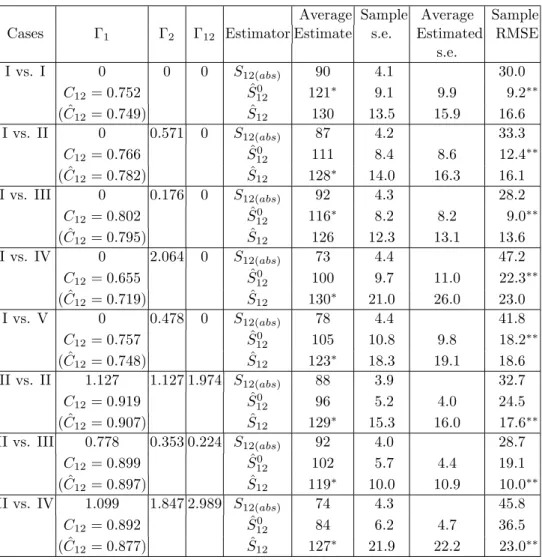
Communities II and IV are in a form of truncated logarithmic series, which is widely prevalent in modeling natural frequency data; see Fisher, Corbet and Williams (1943). It is also called Zipf’s law in linguistics and behavioral sciences. We considered all 15 possible combinations of two communities: I vs. I, I vs. II,. . ., V vs. V as our target communities. Thus we have S₁ = S₂ = 200. Two cases for the number of shared species were selected: S₁₂ = 80 and 120. We assume that the first S₁₂ species are the shared species. In other words, in communities II, III and IV the shared species are the most abundant species whereas in communities I and V the shared ones are equally rare as the unique species. The sample sizes were taken as m₁ =m₂ = 400. Tables 1 and 2 present the simulation results for S₁₂= 120 and 80 respectively.

For each fixed pair of communities, 200 data sets were generated. Each data set consisted of two multinomial samples with 400 individuals in each sample. Then for each generated data set, the observed number of shared species,S_12(obs), was recorded; the estimator ˆS₁₂0 given in (3.11a) and the estimator ˆS₁₂ given in (3.11b) as well as their bootstrap s.e. estimates using 200 replications were obtained. The resulting estimates and s.e.’s were averaged to give the results under the heading “average estimate” and “average estimated s.e.” in Tables 1 and 2. The sample s.e. and sample root mean squared error (RMSE) were also tabulated. The computer program was written in GAUSS and carried out on an IBM RISC 6000 work-station. We also give the values of three CCVs (Γ₁,Γ₂,Γ₁₂), sample coverage (C₁₂) and its estimator ( ˆC₁₂) for the two sub-communities of rare, shared species (as defined in Section 2).

It is evident from the two tables that the observed number of shared species,

S_12(obs), severely underestimates in all cases. It has the largest bias and largest RMSE. Even in the simplest situation (community I vs. I), its bias is substantial. Hence the traditional approach of using S_12(obs) as an estimator of S₁₂ is not

appropriate unless sample sizes are so large that all shared species are observed. Therefore, S_12(obs) will not be included in our following comparison.

When both communities are homogeneous as in the case of I vs. I, all CCVs are zero. The proposed estimator ˆS₁₂0 valid for this homogeneous case performs very well and significantly improves over S_12(obs) in bias and RMSE. When only one community is homogeneous so that two of CCVs are 0, as in the cases of I vs. II, I vs. III, I vs. IV and I vs. V, the estimator ˆS₁₂0 still has the smallest RMSE. This reveals that it is not worthwhile to estimate CCVs in such situations in terms of RMSE. However, when the degree of heterogeneity in the heterogeneous sample is severe, as in the cases of I vs. II, I vs. IV, and I vs. V, the estimator

ˆ

S₁₂ that incorporates estimated CCVs yields smaller or comparable bias. This shows that if one community is homogeneous, we can adopt the use of estimator

ˆ

S₁₂0 unless the other community is highly heterogeneous.

When both communities are heterogeneous (which is the case for virtually any pair of natural communities of species), all CCVs are nonzero. The estimator

ˆ

S₁₂0 that does not consider CCVs is biased downwards, and the magnitude of the bias increases with the magnitude of CCVs. The proposed estimator ˆS₁₂ that takes into account the CCVs can reduce bias but increase the variation due to estimating more parameters. Both tables show that ˆS₁₂generally has the smallest bias and RMSE if community I is not one of the target communities. With respect to RMSE, the estimation of CCVs is warranted because the reduction in bias can compensate for the increase in variation.

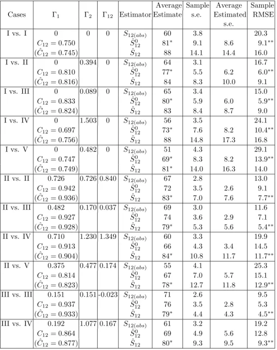
The performance of the estimator ˆS₁₂ clearly depends on the magnitude of CCVs. As in the one-community case, it is usually difficult to estimate CCVs. When all CCVs are large, they cannot be accurately estimated because the species probabilities spread over a wide range. For examples, in the cases of II vs. II, II vs. IV and IV vs. IV in Table 1, as well as the case of IV vs. IV in Table 2, the relatively large CCVs lead to the resulting estimate having larger bias or variation compared with other cases.

Except for the lower sample coverage situations (I vs. IV and IV vs. V), the sample coverage estimator ˆC₁₂ performs well in estimating C₁₂ in both tables. This is exactly the motivation for attempting to estimate the number of shared species using the concept of sample coverage. Note that community IV, where species discovery probability is proportional to 1/i (i.e. π_i ∝1/i), is involved in the two exceptional cases. In community IV, there are only few very frequent species but many infrequent ones. For those few frequent species, if the corre-sponding species probabilities in the other community are relatively small (such as IV vs. I and IV vs. V), then they are likely be missed in the samples. Conse-quently the sample coverage, defined in Equation (3.2), tends to be low. These cases also yield a biased coverage estimator. However, for those few frequent

species in community IV, if the corresponding species probabilities in the other community are also large, as in the cases of IV vs. II, IV vs. III and IV vs. IV, then they would appear in both samples and no problem arises. Generally, when the sample coverage is relatively low (say, lower than 70%), the data provide insufficient information about the number of species in common. In these cir-cumstances, our proposed estimator ˆS₁₂has unavoidably larger bias or variation, although it still has the smallest RMSE and no other competing estimators exist.

Table 1. Comparison of estimators when the true parameter is S₁₂ = 120, m₁=m₂= 400.

S_12(abs): The number of observed shared species; ˆ

S₁₂0: Proposed estimator for the homogeneous cases, see Equation (3.11a); ˆ

S₁₂: Proposed estimator for the heterogeneous cases, see Equation (3.11b).

Average Sample Average Sample

Cases Γ₁ Γ₂ Γ₁₂ Estimator Estimate s.e. Estimated RMSE

s.e. I vs. I 0 0 0 S_12(abs) 90 4.1 30.0 C₁₂= 0.752 Sˆ₁₂0 121∗ 9.1 9.9 9.2∗∗ ( ˆC₁₂= 0.749) Sˆ₁₂ 130 13.5 15.9 16.6 I vs. II 0 0.571 0 S_12(abs) 87 4.2 33.3 C₁₂= 0.766 Sˆ₁₂0 111 8.4 8.6 12.4∗∗ ( ˆC₁₂= 0.782) Sˆ₁₂ 128∗ 14.0 16.3 16.1 I vs. III 0 0.176 0 S_12(abs) 92 4.3 28.2 C₁₂= 0.802 Sˆ₁₂0 116∗ 8.2 8.2 9.0∗∗ ( ˆC₁₂= 0.795) Sˆ₁₂ 126 12.3 13.1 13.6 I vs. IV 0 2.064 0 S_12(abs) 73 4.4 47.2 C₁₂= 0.655 Sˆ₁₂0 100 9.7 11.0 22.3∗∗ ( ˆC₁₂= 0.719) Sˆ₁₂ 130∗ 21.0 26.0 23.0 I vs. V 0 0.478 0 S_12(abs) 78 4.4 41.8 C₁₂= 0.757 Sˆ₁₂0 105 10.8 9.8 18.2∗∗ ( ˆC₁₂= 0.748) Sˆ₁₂ 123∗ 18.3 19.1 18.6 II vs. II 1.127 1.127 1.974 S_12(abs) 88 3.9 32.7 C₁₂= 0.919 Sˆ₁₂0 96 5.2 4.0 24.5 ( ˆC₁₂= 0.907) Sˆ₁₂ 129∗ 15.3 16.0 17.6∗∗ II vs. III 0.778 0.353 0.224 S_12(abs) 92 4.0 28.7 C₁₂= 0.899 Sˆ₁₂0 102 5.7 4.4 19.1 ( ˆC₁₂= 0.897) Sˆ₁₂ 119∗ 10.0 10.9 10.0∗∗ II vs. IV 1.099 1.847 2.989 S_12(abs) 74 4.3 45.8 C₁₂= 0.892 Sˆ₁₂0 84 6.2 4.7 36.5 ( ˆC₁₂= 0.877) Sˆ₁₂ 127∗ 21.9 22.2 23.0∗∗

Table 1. (Continued)

Average Sample Average Sample

Cases Γ₁ Γ₂ Γ₁₂ Estimator Estimate s.e. Estimated RMSE

s.e.

II vs. V 0.546 0.475 0.241 S_12(abs) 76 4.8 44.2

C₁₂= 0.779 Sˆ₁₂0 97 8.9 8.2 25.1

( ˆC₁₂= 0.785) Sˆ₁₂ 121∗ 17.4 18.6 17.4∗∗

III vs. III 0.309 0.309 0.027 S_12(abs) 95 3.7 25.0

C₁₂= 0.908 Sˆ₁₂0 105 5.2 4.1 15.9 ( ˆC₁₂= 0.907) Sˆ₁₂ 115∗ 8.3 8.2 9.7∗∗ III vs. IV 0.393 1.479 0.555 S_12(abs) 77 4.1 43.2 C₁₂= 0.841 Sˆ₁₂0 90 6.7 5.8 30.3 ( ˆC₁₂= 0.842) Sˆ₁₂ 117∗ 16.8 16.6 17.1∗∗ III vs. V 0.177 0.484 0.083 S_12(abs) 80 4.9 40.5 C₁₂= 0.810 Sˆ₁₂0 99 8.1 7.5 22.1 ( ˆC₁₂= 0.804) Sˆ₁₂ 117∗ 13.8 15.0 14.1∗∗ IV vs. IV 2.064 2.064 6.464 S_12(abs) 65 4.3 55.1 C₁₂= 0.888 Sˆ₁₂0 74 6.0 4.7 46.7 ( ˆC₁₂= 0.870) Sˆ₁₂ 128∗ 28.0 29.7 29.2∗∗ IV vs. V 2.028 0.407 -0.131 S_12(abs) 64 4.8 56.3 C₁₂= 0.661 Sˆ₁₂0 89 10.6 11.6 33.1 ( ˆC₁₂= 0.711) Sˆ₁₂ 128∗ 27.9 32.7 28.9∗∗ V vs. V 0.476 0.478 0.227 S_12(abs) 67 5.1 52.9 C₁₂= 0.757 Sˆ₁₂0 89 9.7 8.8 32.8 ( ˆC₁₂= 0.762) Sˆ₁₂ 112∗ 17.2 19.8 19.1∗∗

∗ _{denote the smallest bias;} ∗∗ _{denote the smallest RMSE}

The magnitude of sample coverage also has an impact on the performance of the estimated standard errors based on a bootstrap method as described in the end of Section 3. We can examine the behavior of the estimated s.e. by comparing the estimated s.e. (column 8 in both tables) with the sample stan-dard errors (column 7). Except for the low sample coverage cases, the stanstan-dard error estimates for ˆS₁₂and ˆS₁₂0 using a bootstrap resampling method is generally satisfactory.

In summary, the number of observed shared species in samples severely un-derestimates the true number of shared species. The proposed estimator ˆS₁₂0 for the homogeneous communities is still appropriate if all CCV do not deviate from zero greatly. Otherwise, the estimator ˆS₁₂ incorporating the estimated CCVs can reduce bias and RMSE and can be adopted for practical use.

Table 2. Comparison of estimators when the true parameter is S₁₂ = 80, m₁=m₂= 400.

S_12(abs): The number of observed shared species; ˆ

S₁₂0: Proposed estimator for the homogeneous cases, see Equation (3.11a); ˆ

S₁₂: Proposed estimator for the heterogeneous cases, see Equation (3.11b).

Average Sample Average Sample

Cases Γ₁ Γ₂ Γ₁₂ Estimator Estimate s.e. Estimated RMSE

s.e. I vs. I 0 0 0 S_12(abs) 60 3.8 20.3 C₁₂= 0.750 Sˆ₁₂0 81∗ 9.1 8.6 9.1∗∗ ( ˆC₁₂= 0.745) Sˆ₁₂ 88 14.1 14.4 16.0 I vs. II 0 0.394 0 S_12(abs) 64 3.1 16.7 C₁₂= 0.810 Sˆ₁₂0 77∗ 5.5 6.2 6.0∗∗ ( ˆC₁₂= 0.816) Sˆ₁₂ 84 8.3 10.0 9.1 I vs. III 0 0.089 0 S_12(abs) 65 3.4 15.0 C₁₂= 0.833 Sˆ₁₂0 80∗ 5.9 6.0 5.9∗∗ ( ˆC₁₂= 0.824) Sˆ₁₂ 83 8.4 8.7 9.0 I vs. IV 0 1.503 0 S_12(abs) 56 3.5 24.1 C₁₂= 0.697 Sˆ₁₂0 73∗ 7.6 8.2 10.4∗∗ ( ˆC₁₂= 0.756) Sˆ₁₂ 88 14.8 17.3 16.8 I vs. V 0 0.482 0 S_12(abs) 51 4.3 29.1 C₁₂= 0.747 Sˆ₁₂0 69∗ 8.3 8.2 13.9∗∗ ( ˆC₁₂= 0.749) Sˆ₁₂ 81∗ 14.0 16.3 14.0 II vs. II 0.726 0.726 0.840 S_12(abs) 67 2.8 13.0 C₁₂= 0.942 Sˆ₁₂0 72 3.5 2.6 9.1 ( ˆC₁₂= 0.936) Sˆ₁₂ 83∗ 7.0 7.6 7.7∗∗ II vs. III 0.482 0.170 0.037 S_12(abs) 69 3.0 11.6 C₁₂= 0.927 Sˆ₁₂0 74 3.6 2.9 7.1 ( ˆC₁₂= 0.928) Sˆ₁₂ 79∗ 5.3 5.6 5.4∗∗ II vs. IV 0.710 1.230 1.349 S_12(abs) 60 3.3 19.9 C₁₂= 0.913 Sˆ₁₂0 66 4.3 3.4 14.5 ( ˆC₁₂= 0.904) Sˆ₁₂ 84∗ 10.8 11.7 11.7∗∗ II vs. V 0.375 0.477 0.174 S_12(abs) 55 4.1 25.3 C₁₂= 0.814 Sˆ₁₂0 67 7.0 5.7 15.1 ( ˆC₁₂= 0.823) Sˆ₁₂ 78∗ 12.7 11.8 12.9∗∗

III vs. III 0.151 0.151 -0.023 S_12(abs) 71 2.6 9.5

C₁₂= 0.937 Sˆ₁₂0 76 3.5 2.8 5.3

( ˆC₁₂= 0.933) Sˆ₁₂ 79∗ 4.4 4.3 4.5∗∗

III vs. IV 0.192 1.077 0.167 S_12(abs) 61 3.2 19.2

C₁₂= 0.864 Sˆ₁₂0 69 4.9 5.6 12.8

Table 2. (Continued)

Average Sample Average Sample

Cases Γ₁ Γ₂ Γ₁₂ Estimator Estimate s.e. Estimated RMSE

s.e. III vs. V 0.088 0.481 0.041 S_12(abs) 57 3.6 23.7 C₁₂= 0.832 Sˆ₁₂0 69 5.9 5.6 12.8 ( ˆC₁₂= 0.827) Sˆ₁₂ 78∗ 9.7 10.5 9.9∗∗ IV vs. IV 1.383 1.383 2.934 S_12(abs) 54 3.7 26.0 C₁₂= 0.907 Sˆ₁₂0 60 4.9 3.5 20.7 ( ˆC₁₂= 0.894) Sˆ₁₂ 86∗ 16.2 16.3 17.1∗∗ IV vs. V 1.608 0.386 -0.101 S_12(abs) 49 4.3 31.4 C₁₂= 0.689 Sˆ₁₂0 63 8.3 7.9 18.5 ( ˆC₁₂= 0.758) Sˆ₁₂ 81∗ 16.3 19.8 16.3∗∗ V vs. V 0.460 0.456 0.192 S_12(abs) 46 4.4 34.6 C₁₂= 0.762 Sˆ₁₂0 61 8.0 8.1 20.5 ( ˆC₁₂= 0.750) Sˆ₁₂ 76∗ 14.8 18.1 15.3∗∗

∗ _{denote the smallest bias;} ∗∗ _{denote the smallest RMSE}

5. Real Data Analysis

We refer to Ke-Yar and Chung-Kang estuaries as community I (or area I) and II (or area II), respectively. Totals of m₁ = 85867 and m₂ = 59646 observations have been made from them. In these two areas there were, respectively, 155 and 140 species observed, with 111 of these recorded for both areas (shared species). In our notation, S_1(obs) = 155, S_2(obs) = 140 and S_12(obs) = 111. Now the objective is to estimate the number of unobserved shared species.

First we present the analysis for one community, using area I as an illustra-tion. That is, suppose we have the data only for area I. We estimate the number of species in area I. There are 96 abundant species (each observed more than 10 times) and 59 rare species (each observed 10 times or fewer) in the sample. Using the notation discussed in Section 2, we have S_abun = 96, S_rare = 59 and the first ten order frequency counts are (f₁, . . . , f₁₀) = (25,6,10,3,4,4,1,1,4,1). The sample coverage estimate for the sub-community is ˆC= 1−f₁/10_k=1kf_k= 1−25/184 = 86.4%. If we wrongly regarded the community as homogeneous, then formula (2.1) results in an estimate ˆS0 =S_abun+S_rare/Cˆ = 96 + 59/0.864 = 164. However, the homogenous assumption is not appropriate, as reflected by a large value of CV (ˆγ = 0.768). Therefore, it is necessary to estimate the CV and use the estimator proposed in (2.2). Our estimator yields ˆS=S_abun+Srare

ˆ

C +fCˆ1γˆ2=

in Chao and Lee (1992) produces an estimate of 11. Hence there are about 26 species that were undiscovered in area I. Based on a method suggested by Ken Burnham and presented in Chao (1987), we can construct a 95% confidence interval forS of (167, 213).

Similarly for area II, 59 species were observed 10 times or fewer, and 81 were seen more than 10 times; the first ten frequency counts are 22, 12, 4, 4, 6, 2, 1, 2, 3, 3. Using this information, we obtain an estimate of 163 species (s.e. 10) and a 95% interval of (150, 192).

We now proceed to estimate the number of shared species. Among the observed 111 shared species, there were 90 abundant shared species observed more than 10 times in one or both areas, the other 21 shared species are rare shared species. In our notation, S_12(abun) = 90 and S_12(rare) ≡ M₁₂ = 21. The pairs of frequencies for the 21 “rare shared species” are: (1, 1), (1, 1), (1, 1), (1, 1), (1, 2), (1, 2), (1, 5), (1, 5), (2, 1), (3, 1), (3, 1), (5, 1), (9, 1), (3, 2), (3, 2), (3, 7), (5, 9), (6, 4), (8, 10), (9, 3), and (9, 4). From the data, we havef₁₊ = 8,

f₊₁ = 9 andf₁₁= 4. There are also observed, unique species but we will not list them. The reduced sample sizes (for the sub-community) becomen₁ = 3358 and

n₂ = 558. It follows from Equation (3.5) that the sample coverage estimate is ˆ

C₁₂= 85.97%. If the set of product probabilitiesQ={p₁p∗₁, . . . , p_N

12p∗N12} were homogeneous, the estimator given in (3.6) gives ˆN₁₂0 = 21/0.8597 = 24.43. Thus based on (3.11a), we obtain ˆS₁₂0 =S_12(abun)+ ˆN₁₂0 = 90 + 24 = 114. However, the CCV estimates using (3.9) are ˆΓ₁= 0.7328, Γ₂ = 1.0072 and ˆΓ₁₂= 0.4574. These large values of CCVs show strong evidence for the heterogeneity ofQ. Therefore, we need to incorporate the estimated CCVs in the resulting estimator. Equation (3.10) yields ˆN₁₂= M12 ˆ C12 + 1 ˆ C12[f1+ ˆ Γ₁+f₊₁Γˆ₂+f₁₁Γˆ₁₂] = 24.43 + (0.8579)−1[8× 0.7328 + 9×1.0072 + 4×0.4574] = 44. The proposed estimator of the number of shared species using Equation (3.11b) is ˆS₁₂=S_12(abun)+ ˆN₁₂= 90+44 = 134. A bootstrap s.e. estimate based on 200 bootstrap replications is approximately 20, which implies a 95% confidence interval of (116, 210). We can conclude that there are still 23 shared species not discovered in the survey, with a 95% confidence range of [5, 99].

Acknowledgements

This research was supported by the National Science Council of Taiwan. The bird census data set used in Section 5 was provided by the Wild Bird Society of Hsin-Chu in Taiwan. The authors thank all the “birders” involved in the cen-sus. This valuable data set has enhanced people’s appreciation of our country’s estuaries and bio-diversity. The authors also thank Professor Robert Colwell of University of Connecticut for carefully reading the manuscript and providing thoughtful suggestions and generous editorial help.

References

Bunge, J. and Fitzpatrick, M. (1993). Estimating the number of species: a review. J. Amer. Statist. Assoc. 88, 364-373.

Bunge, J., Fitzpatrick, M. and Handley, J. (1995). Comparison of three estimators of the number of species. J. Appl. Statist. 22, 45-59.

Chao, A. (1987). Estimating the population size for capture-recapture data with unequal catch-ability. Biometrics43, 783-791.

Chao, A. and Lee, S.-M. (1992). Estimating the number of classes via sample coverage. J. Amer. Statist. Assoc. 87, 210-217.

Chao, A., Ma, M.-C. and Yang, M. C. K. (1993). Stopping rules and estimation for recapture debugging with unequal failure rates. Biometrika80, 193-201.

Chen, W.-C. (1980). On the weak form of Zipf’s Law. J. Appl. Probab. 18, 611-622.

Chen, Y.-C., Hwang, W.-H., Chao, A. and Kuo, C.-Y. (1995). Estimating the number of common species - Analysis of the number of common bird species in Ke-Yar Stream and Chung-Kang Stream. J. Chinese Statist. Assoc. 33, 373-393. (in Chinese)

Colwell, R. K. (1973). Competition and coexistence in a simple tropical community. American Naturalist 107, 737-760.

Colwell, R. K. (1997). EstimateS: statistical estimation of species richness and shared species from samples. Version 5. Use’s Guide and Application published at http://viceroy.eeb .uconn.edu/estimates.

Colwell, R. K. and Coddington, J. A. (1994). Estimating terrestrial biodiversity through ex-trapolation. Philos. Trans. Roy. Soc. London Ser. B345, 101-118.

Esty, W. W. (1986). The efficiency of Good’s nonparametric coverage estimator. Ann. Statist. 14, 1257-1260.

Feinsinger, P. (1976). Organization of a tropical guild of nectarivorous birds. Ecological Mono-graphs46, 257-291.

Fisher, R. A., Corbet, A. S. and Williams, C. B. (1943). The relation between the number of species and the number of individuals in a random sample of an animal population. J. Animal Ecology12, 42-58.

Good, I. J. (1953). The population frequencies of species and the estimation of population parameters. Biometrika40, 237-264.

Gower, J. C. (1985). Measures of similarity, dissimilarity, and distance. In Encyclopedia of Statistical Sciences5(Edited by S. Kotz and N. Johnson). Wiley, New York.

Grassle, J. F. and Smith, W. (1976). A similarity measure sensitive to the contribution of rare species and its use in investigation of variation in marine benthic communities. Oecologia 25, 13-22.

Karr, J. R., Robinson, S. K., Blanke, J. G. and Bierregaard, R. O. (1990). Birds of four neotropical forests. In Four Neotropical Rainforests (Edited by A. H. Gentry), 237-269. Yale University Press.

Ludwig, J. A. and Reynolds, J. F. (1988). Statistical Ecology: A Primer on Methods and Computing. Wiley, New York.

Pielou, E. C. (1975). Ecological Diversity. Wiley, New York. Pielou, E. C. (1977). Mathematical Ecology. Wiley, New York.

Seber, G. A. F. (1982),The Estimation of Animal Abundance. 2nd edition. Griffin, London. Seber, G. A. F. (1986). A review of estimating animal abundance. Biometrics42, 267-292. Seber, G. A. F. (1992). A review of estimating animal abundance II.Internat. Statist. Rev.

Institute of Statistics, National Tsing Hua University, Hsin-Chu 30043, Taiwan. E-mail: [email protected]

Wild Bird Society of Hsin-Chu, Hsin-Chu 30043, Taiwan.