Combining progressive hedging with a Frank--Wolfe method to compute Lagrangian dual bounds in stochastic mixed-integer programming

(1)

Research Repository.

The RMIT Research Repository is an open access database showcasing

the research outputs of RMIT University researchers.

RMIT Research Repository:

http://researchbank.rmit.edu.au/

Citation:

See this record in the RMIT Research Repository at:

Version:

Accepted Manuscript

Copyright Statement:

©

Link to Published Version:

https://researchbank.rmit.edu.au/view/rmit:48431

Published Version

2018 Society for Industrial and Applied Mathematics

https://doi.org/10.1137/16M1076290

Boland, N, Christiansen, J, Dandurand, B, Eberhard, A, Linderoth, J and Pinheiro De Oliveira, F 2018, 'Combining Progressive Hedging with a Frank--Wolfe Method to Compute Lagrangian Dual Bounds in Stochastic Mixed-Integer Programming', SIAM Journal of Optimization, vol. 28, no. 2, pp. 1312-1336.

(2)

COMBINING PROGRESSIVE HEDGING WITH A FRANK–WOLFE METHOD TO COMPUTE LAGRANGIAN DUAL BOUNDS IN

STOCHASTIC MIXED-INTEGER PROGRAMMING∗

NATASHIA BOLAND†_{, JEFFREY CHRISTIANSEN}‡_{, BRIAN DANDURAND}‡_,

ANDREW EBERHARD‡_{, JEFF LINDEROTH}§_{, JAMES LUEDTKE}§_, _AND

FABRICIO OLIVEIRA‡

Abstract. We present a new primal-dual algorithm for computing the value of the Lagrangian

dual of a stochastic mixed-integer program (SMIP) formed by relaxing its nonanticipativity con-straints. This dual is widely used in decomposition methods for the solution of SMIPs. The algo-rithm relies on the well-known progressive hedging method, but unlike previous progressive hedging approaches for SMIP, our algorithm can be shown to converge to the optimal Lagrangian dual value. The key improvement in the new algorithm is an inner loop of optimized linearization steps, similar to those taken in the classical Frank–Wolfe method. Numerical results demonstrate that our new algorithm empirically outperforms the standard implementation of progressive hedging for obtaining bounds in SMIP.

Key words. mixed-integer stochastic programming, Lagrangian duality, progressive hedging,

Frank–Wolfe method

AMS subject classifications. 90C06, 90C11, 90C15, 90C46

DOI. 10.1137/16M1076290

1. Introduction. Stochastic programming with recourse provides a framework for modeling problems where decisions are made in stages. Between stages, some uncertainty in the problem parameters is unveiled, and decisions in subsequent stages may depend on the outcome of this uncertainty. When some decisions are modeled using discrete variables, the problem is known as a stochastic mixed-integer program-ming (SMIP) problem. The ability to simultaneously model uncertainty and discrete decisions makes SMIP a powerful modeling paradigm for applications. Important applications employing SMIP models include unit commitment and hydro-thermal generation scheduling [26, 36], military operations [34], vaccination planning [30, 37], air traffic flow management [4], forestry management and forest fire response [6, 28], and supply chain and logistics planning [20, 22]. However, the combination of un-certainty and discreteness makes this class of problems extremely challenging from a computational perspective. In this paper, we present a new and effective algorithm for computing lower bounds that arise from a Lagrangian-relaxation approach.

∗_{Received by the editors May 20, 2016; accepted for publication (in revised form) January 17,}

2018; published electronically May 8, 2018.

http://www.siam.org/journals/siopt/28-2/M107629.html

Funding: The work of authors Boland, Christiansen, Dandurand, Eberhard, Linderoth, and

Oliveira was supported in part or in whole by the Australian Research Council (ARC) grant ARC

DP140100985. The work of authors Linderoth and Luedtke was supported in part by the U.S.

Department of Energy, Office of Science, Office of Advanced Scientic Computing Research, Applied Mathematics program under contract number DE-AC02-06CH11357 and by the NSF under award 1634597.

†_{Georgia Institute of Technology, Atlanta, GA 30332 ([email protected]).}

‡_{RMIT University,} _Melbourne, _Victoria, _{Australia ([email protected],} _brian.

[email protected], [email protected], [email protected]).

§_{Department of Industrial and Systems Engineering, Wisconsin Institutes of Discovery, University}

of Wisconsin-Madison, Madison, WI 53706 ([email protected], [email protected]). 1312

(3)

The mathematical statement of a two-stage SMIP is (1) ζSM IP := min

x

c>x+Q(x) : x∈X ,

where the vector c ∈ Rnx _{is known, and} _X _{is a mixed-integer linear set consisting}

of linear constraints and integer restrictions on some components ofx. The function Q:_Rnx_7→

Ris the expected recourse value Q(x) :=Eξ min y q(ξ)>y : W(ξ)y=h(ξ)−T(ξ)x, y∈Y(ξ) .

We assume that the random variable ξis taken from a discrete distribution indexed by the finite setS, consisting of the realizations,ξ1, . . . , ξ|S|, corresponding to strictly positive probabilities of realization, p1, . . . , p|S|. When ξis not discrete, a finite sce-nario approximation can be obtained via Monte Carlo sampling [19, 24] or other methods [11, 10]. Each realization ξs of ξ is called ascenario and encodes the

real-izations observed for each of the random elements (q(ξs), h(ξs), W(ξs), T(ξs), Y(ξs)).

For notational brevity, we refer to this collection of random elements respectively as (qs, hs, Ws, Ts, Ys). For eachs∈ S, the setYs⊂Rny _{is a mixed-integer set containing}

both linear constraints and integrality constraints on a subset of the variablesys.

The problem (1) may be reformulated as adeterministic equivalent

(2) ζSM IP = min x,y c>x+X s∈S psqs>ys : (x, ys)∈Ks∀s∈ S ,

whereKs:={(x, ys) : Wsys=hs−Tsx, x∈X, ys∈Ys}. Problem (2) has a special

structure that can be algorithmically exploited by decomposition methods. To induce a decomposable structure, scenario-dependent copiesxs for each s∈ S of the

first-stage variablexare introduced to create the following reformulation of (2): (3) ζSM IP = min x,y,z X s∈S ps(c>xs+q>sys) : (xs, ys)∈Ks, xs=z ∀s∈ S, z∈Rnx .

The constraints xs = z, s ∈ S, enforce nonanticipativity for first-stage decisions;

the first-stage decisionsxs must be the same (z) for each scenarios ∈ S. Applying

Lagrangian relaxation to the nonanticipativity constraints in problem (3) yields the

nonanticipative Lagrangian dual function

(4) φ(µ) := min x,y,z P s∈S ps(c>xs+qs>ys) +µ>s(xs−z) : (xs, ys)∈Ks∀s∈ S, z∈Rnx ,

where µ= (µ1, . . . , µ|S|)∈Qs∈SRnx is the vector of multipliers associated with the relaxed constraintsxs=z,s∈ S. By settingωs:= _p1_sµs, (4) may be rewritten as

(5) φ(ω) := min x,y,z ( X s∈S psLs(xs, ys, z, ωs) : (xs, ys)∈Ks∀s∈ S, z∈Rnx ) , where Ls(xs, ys, z, ωs) :=c>xs+qs>ys+ωs>(xs−z).

Sincezis unconstrained in the optimization problem in the definition (5), in order for the Lagrangian function φ(ω) to be bounded from below, we require as a condition

(4)

of dual feasibility that P

s∈Spsωs= 0. Under this assumption, thez term vanishes,

and the Lagrangian dual function (5) decomposes into separable functions,

(6) φ(ω) =X

s∈S

psφs(ωs),

where for eachs∈ S,

(7) φs(ωs) := min x,y

(c+ωs)>x+q>sy : (x, y)∈Ks .

The reformulation (6) is the basis for parallelizable approaches for computing dual bounds that are used, for example, in the dual decomposition methods developed in [9, 23].

For any choice of ω = (ω1, . . . , ω|S|), it is well known that the value of the Lagrangian dual function provides a lower bound on the optimal solution to (1):

φ(ω)≤ζSM IP_{. The problem of finding the best such lower bound is the}_Lagrangian

dual problem: (8) ζLD:= sup ω ( φ(ω) : X s∈S psωs= 0 ) .

The primary contribution of this work is a new and effective method for solving (8), thus enabling a practical and efficient computation of high-quality lower bounds for

ζSM IP.

The function φ(ω) is a piecewise-affine concave function, and many methods are known for maximizing such functions. These methods include the subgradient method [35], the augmented Lagrangian (AL) method [16, 31], and the alternating direction method of multipliers (ADMM) [14, 12, 8]. The subgradient method has mainly theoretical significance, since it is difficult to develop reliable and efficient step-size rules for the dual variablesω (see, e.g., section 7.1.1 of [33]). As iterative primal-dual approaches, methods based on the AL method or ADMM are more effective in practice. However, in the context of SMIP, both methods require convexification of the constraintsKs,s∈ S, to have a meaningful theoretical support for convergence to

the best lower bound valueζLD_{. Furthermore, both methods require the solution of}

additional mixed-integer linear programming (MILP) subproblems in order to recover the Lagrangian lower bounds associated with the dual values,ω [15]. ADMM has a more straightforward potential for decomposability and parallelization than the AL method, and so in this work we develop a theoretically supported modification of a method based on ADMM.

When specialized to the deterministic equivalent problem (2) in the context of stochastic programming, ADMM is referred to as progressive hedging (PH) [32, 39]. When the sets Ks, s ∈ S, are convex, the limit points of the sequence of

solution-multiplier pairs

((xk_{, y}k_{, z}k₎_{, ω}k₎ ∞

k=1 generated by PH are saddle points of the de-terministic equivalent problem (2), whenever such saddle points exist. When the constraints (xs, ys)∈Ks,s∈ S, enforce nontrivial mixed-integer restrictions, the set

Ks is not convex and PH becomes a heuristic approach with no guarantees of

con-vergence [21]. Nevertheless, some measure of success in practice has been observed in [39] while applying PH to problems of the form (3). More recently, [15] showed that valid Lagrangian lower bounds can be calculated from the iterates of the PH algorithm when the sets Ks are not convex. However, their implementation of the

(5)

algorithm does not offer any guarantee that the lower bounds will converge to the optimal value ζLD_{. Moreover, additional computational effort, in solving additional}

MILP subproblems, must be expended in order to compute the lower bound. Our contribution is to extend the PH-based approach in [15], creating an algorithm whose lower bound values converge toζLD_{in theory and for which lower bound calculations}

do not require additional computational effort. Computational results in section 4 demonstrate that the new method outperforms the existing PH-based method, in terms of both quality of bound and efficiency of computation.

To motivate our approach, we first consider the application of PH to the following well-known primal characterization ofζLD:

(9) ζLD= min x,y,z ( X s∈S ps(c>xs+q>sys) : (xs, ys)∈conv(Ks), xs=z ∀s∈ S ) ,

where conv(Ks) denotes the convex hull of Ks for each s ∈ S. (See, for example,

Theorem 6.2 of [25].)

The sequence of Lagrangian bounds{φ(ωk₎_}_{generated by the application of PH}

to (9) is known to be convergent. Thus, the value of the Lagrangian dual problem (ζLD_{) may, in theory, be computed by applying PH to (9). However, in practice, an}

explicit polyhedral description of conv(Ks), s ∈ S, is generally not available, thus

raising the issue of implementability.

The absence of such an explicit description motivates an application of a solu-tion approach to the PH primal update step that iteratively constructs an improved inner approximation of each conv(Ks),s∈ S. For this purpose, we apply a solution

approach to the PH primal update problem that is based on the Frank–Wolfe (FW) method [13]. Our approach has the additional benefit of providing Lagrangian bounds at no additional computational cost.

One simple, theoretically supported integration of an FW-like method and PH is realized by having the PH primal updates computed using a method called the simpli-cial decomposition method (SDM) [17, 38]. SDM is an extension of the FW method that makes use of progressively improving inner approximations to each set conv(Ks),

s ∈ S. The finite optimal convergence of each application of SDM follows directly from the polyhedral structure conv(Ks) and the (practically reasonable) assumption

that conv(Ks) is bounded for each s∈ S.

For computing improvements in the Lagrangian bound efficiently, convergence of SDM to the optimal solution of the subproblem is too costly and not necessary. We thus develop a modified integration whose theoretically supported convergence analysis is based not on the optimal convergence of SDM, but rather on its ability to adequately extend the inner approximations of each conv(Ks),s∈ S.

The main contribution of this paper is the development, convergence analysis, and application of a new algorithm, called FW-PH, which is used to compute high-quality Lagrangian bounds for SMIPs efficiently and with a high potential for parallelization. FW-PH is efficient in that, under mild assumptions, each dual update and Lagrangian bound computation may be obtained by solving, for eachs∈ S, just one MILP prob-lem and one continuous convex quadratic probprob-lem. In contrast, each dual update of PH requires the solution of a mixed-integer quadratic programming (MIQP) subprob-lem for eachs∈ S, and each PH Lagrangian bound computation requires the solution of one MILP subproblem for eachs∈ S. In our convergence analysis, conditions are provided under which the sequence of Lagrangian bounds generated by FW-PH con-verges to the optimal Lagrangian bound ζLD_{. To the best of our knowledge, the}

(6)

combination of PH and FW in a manner that is theoretically supported, computa-tionally efficient, and parallelizable is new, in spite of the convergence analyses of both PH and FW being well developed. We also perform an experimental assessment of alternative heuristic strategies that can be employed in a straightforward manner to recover feasible solutions for problem (3) from the solution obtained by FW-PH for problem (9).

This paper is organized as follows. In section 2, we present the theoretical back-ground of PH and a brief technical lemma regarding the inner approximations gener-ated by SDM; this background is foundational to the proposed FW-PH method. In section 3, we present the FW-PH method and a convergence analysis. We also present in this section heuristic strategies that can be employed to generate primal feasible first-stage solutions. The results of numerical experiments comparing the Lagrangian bounds computed with PH and those with FW-PH are presented in section 4. We also provide a comparison of the primal solutions obtained employing the heuristics described. We conclude in section 5 with a discussion of the results obtained and with suggested directions for further research.

2. Progressive hedging and Frank–Wolfe-based methods. Theaugmented Lagrangian (AL) dual function based on the relaxation of the nonanticipativity con-straintsxs=z,s∈ S, is Lρ(x, y, z, ω) :=X s∈S psLρs(xs, ys, z, ωs), where Lρ_s(xs, ys, z, ωs) :=c>xs+q>sys+ωs>(xs−z) + ρ 2kxs−zk 2 2

and ρ > 0 is a penalty parameter. By changing the feasible region, denoted here by Ds, s ∈ S, the AL dual problem (i.e., the Lagrangian dual problem in which

the Lagrangian dual function is replaced by its augmented version) can be used in a progressive hedging (PH) approach to solve either problem (3) or problem (9). Pseudocode for the PH algorithm is given in Algorithm 1.

In Algorithm 1, kmax > 0 is the maximum number of iterations and > 0

parameterizes the convergence tolerance. The initialization of lines 3–8 provides an initial target primal valuez0and dual valuesω1_s,s∈ S, for the main iterationsk≥1. Also, an initial Lagrangian boundφ0 can be computed from this initialization.

For > 0, the Algorithm 1 termination criterion

q P

s∈Spskxks−zk−1k

2 2 < is motivated by the addition of the squared norms of the primal and dual residuals associated with problem (9). These residuals, as developed in section 3.3 of [8] within the more general context of ADMM, are measures of how close (xk_{, y}k_{, z}k_{) come}

to satisfying the necessary and sufficient conditions of optimality for problem (9). Hence, we enforce an adequate vanishing of primal and dual feasibility residuals, which ultimately implies the vanishing of primal (and dual) objective value suboptimality [8]. In summing the squared norm primal residualspskxks−zkk22,s∈ S, and the squared norm dual residualkzk₋_zk−1_k2

2, we have (10) X s∈S ps h xk_s−zk 2 2+ zk−zk−1 2 2 i =X s∈S ps xk_s−zk−1 2 2.

The equality in (10) follows since, for each s∈ S, the cross term resulting from the expansion of the squared normk(xk

s−zk) + (zk−zk−1)k22vanishes; this is seen in the equalityP

s∈Sps(xks−zk) = 0 due to the construction ofzk.

(7)

Algorithm 1PH applied to problem (3) (Ds=Ks) or (9) (Ds= conv(Ks)). 1: Precondition: P s∈Spsωs0= 0 2: function_PH(ω0_,_ρ_, _k max,) 3: fors∈ S do 4: (x0 s, ys0)∈argminx,y (c+ω0 s)>x+qs>y : (x, y)∈Ds 5: end for 6: φ0←P s∈Sps (c+ω0s)>x0s+qs>ys0 7: z0←P s∈Spsx0s 8: ωs1←ω0s+ρ(x0s−z0) for alls∈ S 9: fork= 1, . . . , kmax do 10: fors∈ S do 11: φk s←minx,y (c+ωk s)>x+q>sy : (x, y)∈Ds 12: (xk_s, y_sk)∈argmin_x,yLρ_s(x, y, zk−1, ωk_s) : (x, y)∈Ds 13: end for 14: φk ←P s∈Spsφks 15: zk_←P s∈Spsxks 16: if q P s∈Spskxks−zk−1k 2 2< then 17: return (xk, yk, zk, ωk, φk) 18: end if 19: ωk+1 s ←ωsk+ρ(xks−zk) for alls∈ S 20: end for

21: return (xkmax_{, y}kmax_{, z}kmax_{, ω}kmax_{, φ}kmax₎ 22: end function

The line 11 subproblem of Algorithm 1 is an addition to the original PH algorithm. Its purpose is to compute Lagrangian bounds (line 14) from the current dual solution

ωk[15]. Thus, the bulk of computational effort in Algorithm 1 applied to problem (3) (the case with Ds =Ks) resides in computing solutions to the MILP (line 11) and

MIQP (line 12) subproblems. Note that line 11 (and line 14) may be omitted if the corresponding Lagrangian bound forωk _{is not desired.}

2.1. Convergence of PH. The following proposition addresses the convergence of PH applied to problem (9).

Proposition 2.1. Assume that problem (9) is feasible with conv(Ks) bounded

for eachs∈ S, and let Algorithm1be applied to problem (9)(so thatDs= conv(Ks)

for eachs∈ S) with tolerance= 0 for eachk≥1. Then, the limitlimk→∞ωk=ω∗

exists and, furthermore,

1. limk→∞Ps∈Sps(c>xks+qs>y k s) =ζ

LD_,

2. limk→∞φ(ωk) =ζLD,

3. limk→∞(xks−zk) = 0for each s∈ S,

and each limit point(((x∗_s, y∗_s)s∈S, z∗)is an optimal solution for (9).

Proof. Since the constraint setsDs = conv(Ks), s∈ S, are bounded, and

prob-lem (9) is feasible, probprob-lem (9) has an optimal solution ((x∗_s, y∗_s)s∈S, z∗) with optimal valueζLD_{. The feasibility of problem (9), the linearity of its objective function, and}

the bounded polyhedral structure of its constraint set Ds= conv(Ks),s∈ S, imply

that the hypotheses for PH convergence to the optimal solution are met (See Theorem 5.1 of [32]). Therefore,ωk _{converges to some}_ω∗_{, lim}

k→∞Ps∈Sps(c>xks+q>sys) =

(8)

ζLD_{, lim}

k→∞φ(ωk) =ζLD, and limk→∞(xks−zk) = 0 for each s∈ S all hold. The

boundedness of eachDs= conv(Ks),s∈ S, furthermore implies the existence of limit

points ((x∗_s, y∗_s)s∈S, z∗) of{((xks, yks)s∈S, zk)}, which are optimal solutions for (9). Note that the convergence in Proposition 2.1 applies to the continuous problem (9) but not to the mixed-integer problem (3). In problem (3), the constraint sets Ks,

s∈ S, are not convex, so there is no guarantee that Algorithm 1 will converge when applied to (3). However, the application of PH to problem (9) requires, in line 12, the optimization of the AL over the sets conv(Ks),s∈ S, for which an explicit linear

description is unlikely to be known. In the next section, we demonstrate how to circumvent this difficulty by constructing inner approximations of the polyhedral sets conv(Ks),s∈ S.

2.2. A Frank–Wolfe approach based on simplicial decomposition. To use Algorithm 1 to solve (9) requires a method for solving the subproblem

(11) (xk_s, y_sk)∈argmin

x,y

Lρ_s(x, y, zk−1, ω_sk) : (x, y)∈conv(Ks)

appearing in line 12 of the algorithm. Although an explicit description of conv(Ks)

is not readily available, if we have a linear objective function, then we can replace conv(Ks) withKs(solving one MIP problem per scenario). This motivates the

appli-cation of an FW algorithm for solving (11), since the FW algorithm solves a sequence of problems in which the nonlinear objective is linearized using a first-order approxi-mation.

The simplicial decomposition method (SDM) is an extension of the FW method, where the line searches of FW are replaced by searches over polyhedral inner approx-imations. SDM can be applied to solve a feasible, bounded problem of the general form

(12) ζF W := min

x {f(x) :x∈D},

with nonempty compact convex setDand continuously differentiable convex function

f. Generically, given a current solution xt−1 and inner approximation Dt−1 ⊆ D, iterationtof the SDM consists of solving

b

x∈argmin

x

∇xf(xt−1)>x:x∈D ,

updating the inner approximation asDt←conv(Dt−1∪ {x_b}), and finally choosing

xt∈argmin

x

f(x) :x∈Dt .

The algorithm terminates when the bound gap is small, specifically, when Γt:=−∇xf(xt−1)>(x_b−xt−1)≤τ,

whereτ ≥0 is a given tolerance.

The application of SDM to solve problem (11), i.e., to minimize Lρ

s(x, y, z, ωs)

over (x, y) ∈ conv(Ks) for a given s ∈ S, is presented in Algorithm 2. Here, tmax

is the maximum number of iterations and τ > 0 is a convergence tolerance. Γt _is

the bound gap used to measure closeness to optimality, and φs is used to compute

a Lagrangian bound as described in the next section. The inner approximation to

(9)

Algorithm 2SDM applied to problem (11). 1: Precondition: V0 s ⊂conv(Ks) andz=P_s_∈Spsx0s 2: functionSDM(V0 s,x0s,ωs,z,tmax,τ) 3: fort= 1, . . . , tmax do 4: ω_bt s←ωs+ρ(xts−1−z) 5: (x_bs,_bys)∈argminx,y (c+ω_bt_s)>x+q_s>y : (x, y)∈ V(conv(Ks)) 6: if t= 1 then 7: φs←(c+ωb t s)>xbs+q > sbys 8: end if 9: Γt← −[(c+ω_bts)>(bxs−x t−1 s ) +q>s(ybs−y t−1 s )] 10: Vt s ←Vst−1∪ {(xbs,bys)} 11: (xt

s, yts)∈argminx,y{Lρs(x, y, z, ωs) : (x, y)∈conv(Vst)}

12: if Γt_≤_τ _then 13: return (xt s, yst, Vst, φs) 14: end if 15: end for 16: return (xtmax s , ytsmax, Vstmax, φs) 17: end function

conv(Ks) at iterationt≥1 takes the form conv(Vst), whereVstis a finite set of points

withVt

s ⊂conv(Ks). The points added by Algorithm 2 to the initial set,Vs0, to form

Vt

s are all inKs: here V(conv(Ks)) is the set of extreme points of conv(Ks) and, of

course,V(conv(Ks))⊆Ks. Observe that ∇(x,y)Lρs(x, y, z, ωs)|(x,y)=(xt−s 1,yst−1) = c+ωs+ρ(xts−1−z) qs = c+ω_bs qs ,

withω_bs=ωs+ρ(xts−1−z), and so the optimization at line 5 is minimizing the gradient

approximation to Lρ

s(x, y, z, ωs) at the point (xts−1, yst−1). Since this is a linear

ob-jective function, optimization overV(conv(Ks)) can be accomplished by optimization

overKs (see, e.g., section I.4, Theorem 6.3 of [25]). Hence line 5 requires a solution

of a single-scenario MILP.

The optimization at line 11 can be accomplished by expressing (x, y) as a convex combination of the finite set of points,Vt

s, where the weightsa∈R|V

t

s|in the convex

combination are now also decision variables. That is, the line 11 problem is solved with a solution to the following convex continuous quadratic subproblem:

(13) (xt_s, yt_s, a)∈argmin x,y,a ( Lρs(x, y, z, ωs) : (x, y) =P(ˆxi_,_ˆ_yi_)∈_Vt sai(ˆx i_,_y_ˆi₎_, P i=1,...,|Vt s|ai= 1, andai≥0 fori= 1, . . . ,|V t s| ) .

For implementational purposes, the x and y variables may be substituted out of the objective of problem (13), leavinga as the only decision variable, with the only constraints being nonnegativity of thea components and the requirement that they sum to 1.

SDM is known to terminate finitely with an optimal solution whenDis polyhedral [17], so the primal update step line 12, Algorithm 1 with Ds = conv(Ks) could be

accomplished with SDM, resulting in an algorithm that converges to a solution to problem (9). This solution, despite not being feasible for problem (3) in general (as it

(10)

typically does not observe integrality requirements), gives the Lagrangian dual bound

ζLD_{. However, since each inner iteration of line 5, Algorithm 2 requires the solution of}

a MILP, usingtmax large enough to ensure SDM terminates optimally is not efficient for our purpose of computing Lagrangian bounds. In the next section, we give an adaptation of the algorithm that requires the solution of onlyoneMILP subproblem per scenario at each major iteration of the PH algorithm.

3. The FW-PH method. In order to make SDM efficient when used with PH to solve problem (9), the minimization of the augmented Lagrangian dual problem can be solved approximately. This insight can greatly reduce the number of MILP subproblems solved at each inner iteration and forms the basis of our algorithm FW-PH. Convergence of FW-PH relies on the following lemma, which states an important expansion property of the inner approximations employed by SDM.

Lemma 3.1. For any scenario s ∈ S and iteration k ≥ 1, let Algorithm 2 be applied to the minimization problem (11)for any tmax≥2. For 1≤t < tmax, if

(14) (xt_s, yt_s)6∈argmin

x,y

Lρ_s(x, y, zk−1, ω_sk) : (x, y)∈conv(Ks)

holds, thenconv(Vt+1

s )⊃conv(Vst).

Proof. Fors∈ S andk≥1 fixed, we know that by construction (xt_s, yt_s)∈argmin

x,y

Ls_ρ(x, y, zk−1, ω_sk) : (x, y)∈conv(V_st)

for t ≥ 1. Given the convexity of (x, y) 7→ Ls

ρ(x, y, zk−1, ωks) and the convexity of

conv(Vt

s), the necessary and sufficient condition for optimality

(15) ∇(x,y)Lsρ(x t s, y t s, z k−1_{, ω}k s) x−xt_s y−yts

≥0 for all (x, y)∈conv(V_st)

is satisfied. By assumption, condition (14) is satisfied, conv(Ks) is likewise convex,

and so the resultingnonsatisfaction of the necessary and sufficient condition of opti-mality for the problem in (14) takes the form

(16) min x,y ∇(x,y)Lsρ(x t s, y t s, z k−1_{, ω}k s) x−xt s y−yt_s : (x, y)∈conv(Ks) <0.

In fact, during SDM iteration t+ 1, an optimal solution (_bxs,ybs) to the problem in

condition (16) is computed in line 5 of Algorithm 2. Therefore, by the satisfaction of condition (15) and the optimality of (_bxs,ybs) for the problem of condition (16), which

is also satisfied, we have (x_bs,bys)6∈conv(V t

s). By construction,Vst+1←Vst∪{(bxs,ybs)},

so that conv(Vt+1

s )⊃conv(Vst) must hold.

3.1. Convergence of FW-PH. The FW-PH algorithm is stated in pseudocode form in Algorithm 3. Similar to Algorithm 1, the parameteris a convergence toler-ance, andkmaxis the maximum number of (outer) iterations. The parametertmaxis

the maximum number of (inner) SDM iterations in Algorithm 2.

The parameterα∈_Raffects the initial linearization point ˜xsof the SDM method.

Any value α∈ R may be used, but the use of ˜xs = (1−α)zk−1+αxks−1 in line 6

is a crucial component in the efficiency of the FW-PH algorithm, as it enables the computation of a valid dual bound,φk_{, at}_each _{iteration of FW-PH without the need}

for additional MILP subproblem solutions. Specifically, we have the following result.

(11)

Algorithm 3FW-PH applied to problem (9). 1: function_FW-PH((V0 s)s∈S, (x0s, y0s)s∈S, ω0,ρ,α,,kmax, tmax) 2: z0_←P s∈Spsx0s 3: ω1 s ←ω0s+ρ(x0s−z0) fors∈ S 4: fork= 1, . . . , kmax do 5: fors∈ S do 6: _exs←(1−α)zk−1+αxks−1 7: [xks, yks, Vsk, φsk]←SDM(Vsk−1,xes, ω k s, zk−1, tmax,0) 8: end for 9: φk ←P_s_∈Spsφks 10: zk_←P s∈Spsxks 11: if q P s∈Spskxks−zk−1k 2 2< then 12: return ((xk s, yks)s∈S, zk, ωk, φk) 13: end if 14: ωk+1 s ←ωsk+ρ(xks−zk) fors∈ S 15: end for 16: return (xkmax

s , yskmax)s∈S, zkmax), ωkmax, φkmax

17: end function

Proposition 3.2. Assume that the precondition P

s∈Spsω0s = 0holds for

Algo-rithm3. At each iteration k≥1of Algorithm3, the value,φk_{, calculated at line}₉_{, is}

the value of the Lagrangian dual functionφ(·)evaluated at a Lagrangian dual feasible point, and hence provides a finite lower bound onζLD_.

Proof. SinceP

s∈Spsωs0 = 0 holds and, by construction, 0 = P

s∈Sps(x0s−z0),

we haveP

s∈Spsω1s= 0 also. We proceed by induction onk≥1. At iterationk, the

problem solved for eachs∈ Sat line 5 in the first iteration (t= 1) of Algorithm 2 may be solved with the same optimal value by exchangingV(conv(Ks)) forKs; this follows

from the linearity of the objective function. Thus, an optimal solution computed at line 5 may be used in the computation ofφs(ω_esk) carried out in line 7, where

e ω_sk:=ω_b1_s=ω_sk+ρ(x_es−zk−1) =ωsk+ρ((1−α)z k−1₊_αxk−1 s −z k−1₎ =ω_sk+αρ(x_sk−1−zk−1).

By construction, we have at each iterationk≥1 in Algorithm 3 that

X s∈S ps(xks−1−z k−1_{) = 0} _and X s∈S psωsk = 0,

which establishes that P s∈Spsωe

k

s = 0. Thus, ωe

k _{is feasible for the Lagrangian dual}

problem, so that φ(ω_ek) = P

s∈Spsφks, and, since each φks is the optimal value of a

bounded and feasible mixed-integer linear program, we have−∞< φ(ω_ek₎_<_∞_.

We establish convergence of Algorithm 3 for anyα∈ Rand tmax ≥1. For the

special case in which we perform only one iteration of SDM for each outer iteration (tmax= 1), we require the additional assumption that the initial scenario vertex sets

share a common point. More precisely, we require the assumption

(17) \

s∈S

Proj_x(conv(V_s0))6=∅,

(12)

which can, in practice, be effectively handled through appropriate initialization, under the standard assumption of relatively complete recourse: for all x ∈ X and s ∈ S there exists ys such that (x, ys)∈Ks. We describe one such initialization approach

in section 4.

Proposition 3.3. Let the convexified separable deterministic equivalent SMIP

(9) have an optimal solution, and let Algorithm3 be applied to (9) with kmax=∞,

= 0,α∈R, andtmax≥1. If eithertmax≥2or (17)holds, thenlimk→∞φk=ζLD.

Proof. First note that for any tmax ≥ 1 the sequence of inner approximations

conv(Vk

s), s ∈ S, will stabilize in that, for some threshold 0 ≤k¯s, we have, for all

k≥k¯s,

(18) conv(V_sk) =:Ds⊆conv(Ks).

This follows due to the assumption that each expansion of the inner approxima-tions conv(Vk

s) takes the form Vsk ←Vsk−1∪ {(xbs,bys)}, where (bxs,bys) is a vertex of

conv(Ks). Since each polyhedron conv(Ks), s∈ S, has only a finite number of such

vertices, the stabilization (18) must occur at some ¯ks<∞.

For tmax ≥2, the stabilizations (18), s∈ S, are reached at some iteration ¯k := maxs∈S¯ks . Noting thatDs= conv(Vsk) fork > kwe must have

(19) (xk_s, y_sk)∈argmin

x,y

Lρ_s(x, y, zk−1, ω_sk) : (x, y)∈conv(Ks) .

Otherwise, due to Lemma 3.1, the call to SDM on line 7 must return Vk

s ⊃ Vsk−1,

contradicting the finite stabilization (18). Therefore, the k ≥ ¯k iterations of Algo-rithm 3 are identical to AlgoAlgo-rithm 1 iterations, and so Proposition 2.1 implies that limk→∞xks−zk = 0,s∈ S, and limk→∞φ(ωk) =ζLD. By the continuity ofω7→φs(ω)

for each s ∈ S, we have limk→∞φk = limk→∞Ps∈Spsφs(ωsk+α(xks−1−zk−1)) =

limk→∞Ps∈Spsφs(ωks) = limk→∞φ(ωk) =ζLD for allα∈R.

In thetmax= 1 case, we have at each iterationk≥1 the optimality

(xk_s, yk_s)∈argmin

x,y

Lρ_s(xs, ys, zk−1, ωsk) : (xs, ys)∈conv(Vsk) .

By the definition of stabilization (18), the iterationsk≥¯kof Algorithm 3 are identical to PH iterations applied to the restricted problem

(20) min x,y,z ( X s∈S ps(c>xs+qs>ys) : (xs, ys)∈Ds∀s∈ S, xs=z∀s∈ S ) .

We have initialized the sets (Vs0)s∈S such that ∩s∈SProjxconv(Vs0) 6= ∅, so since

the inner approximations to conv(Ks) only expand in the algorithm, we have that

∩s∈SProjx(Ds) 6= ∅. Therefore, problem (20) is a feasible and bounded linear

program, and so the PH convergence described in Proposition 2.1 with Ds = Ds,

s ∈ S holds for its application to problem (20). That is, for each s ∈ S, we have (1) limk→∞ωks = ωs∗ and limk→∞(xks −zk) = 0; and (2) for all limit points

((x∗_s, y_s∗)s∈S, z∗), we have the feasibility and optimality of the limit points, which impliesx∗_s=z∗ and

(21) min

x,y

(c+ω∗_s)>(x−x∗) +q>_s(y−y∗) : (x, y)∈Ds = 0.

(13)

Next, for each s ∈ S the compactness of conv(Ks) ⊇ Ds, the continuity of the

minimum value function

ω7→min x,y (c+ω)>x+qs>y : (x, y)∈Ds overω∈ ω : P

s∈Spsωs= 0 , and the limit limk→∞ωe k+1

s = limk→∞ωsk+1+αρ(xks−

zk_{) =}_ω∗

s, together imply that

(22) lim k→∞minx,y (c+_eω_sk+1)>(x−xk) +q_s>(y−yk) : (x, y)∈Ds = 0. Recall that _eωk s =ωsk+ρα(xsk−1−zk−1) is thet = 1 value ofωb t sdefined in line 4 of

Algorithm 2. Thus, fork+ 1>¯k, we have due to the stabilization (18) that (23) min x,y (c+_eωk_s+1)>(x−xk) +q_s>(y−yk) : (x, y)∈Ds = min x,y (c+ω_ek_s+1)>(x−xk) +q>_s(y−yk) : (x, y)∈conv(Ks)

If (23) does not hold, then the inner approximation expansionDs⊂conv(Vsk+1) must

occur, since a point (x_bs,_bys)∈conv(Ks) that can be strictly separated fromDswould

have been discovered during the iterationk+ 1 execution of Algorithm 2, line 5,t= 1. The expansionDs⊂conv(Vsk+1) contradicts the finite stabilization (18), and so (23)

holds. Therefore, the equalities (22) and (23) imply that (24) lim

k→∞minx,y

(c+ω_e_sk+1)>(x−xk) +q>_s(y−yk) : (x, y)∈conv(Ks) = 0.

Our argument has shown that for all limit points (x∗_s, y∗_s), s ∈ S, the stationarity condition

(25) (c+ω∗_s)>(x−x∗_s) +q_s>(y−y∗_s)≥0 ∀(x, y)∈conv(Ks)

is satisfied, which together with the feasibility x∗_s = z∗, s ∈ S, implies that each limit point ((x∗_s, y_s∗)s∈S, z∗) is optimal for problem (9) andω∗is optimal for the dual problem (8).

Thus, for all tmax ≥1, we have shown that limk→∞(xks −zk) = 0, s ∈ S, and

limk→∞φ(ωk) =ζLD. By similar reasoning to that used in the tmax ≥2 case, it is

straightforward that, for allα∈R, we also have limk→∞φk=ζLD.

While using a large value oftmaxmore closely matches Algorithm 3 to the original

PH algorithm as described in Algorithm 1, we are motivated to use a small value of

tmax since the work per iteration is proportional to tmax. Specifically, each iteration

requires solvingtmax|S|MILP subproblems andtmax|S|continuous convex quadratic

subproblems. For reference, Algorithm 1 applied to problem (3) requires the solution of |S| MIQP subproblems for each ω update and |S| MILP subproblems for each Lagrangian boundφcomputation.

3.2. Obtaining primal feasible solutions. As the FW-PH algorithm is de-signed to solve (9) (which is an optimization over conv(Ks) rather than Ks), any

solution it returns at convergence may not satisfy the integrality requirements and hence may not be primal feasible. Nevertheless, the information returned by FW-PH at termination may be exploited heuristically to derive primal feasible solutions. We suggest two simple heuristic strategies which use the solution ((xk

s, ysk)s∈S, zk, ωk)

(14)

returned by FW-PH, as defined in Algorithm 3. These strategies may be used regard-less of whether or not convergence has been achieved at termination. Both strategies take advantage of the assumption of relatively complete recourse: They evaluate a candidate first-stage solution by solving each of the|S|single-scenario problems with its first-stage variables fixed to the candidate values.

The first heuristic strategy, which we call H1, consists of evaluating each distinct solution in the set of solutions {x_bk_s :s∈ S}, obtained in the last execution of line 7 of Algorithm 3, as a candidate first-stage solution.

The second strategy, H2, consists of solving the MIQPs, one for eachs∈ S, that would have been solved in PH (line 12 in Algorithm 1) usingz =zk, ω =ωk, and consideringDs=Ksfors∈ S, and evaluating each distinct first-stage solution found.

Notice that either strategy may generate multiple candidate first-stage solutions, in particular when the FW-PH convergence criterion is not met at termination. In this case, the one evaluated to yield the best objective function value is selected. In section 4, we provide numerical results that assess the performance of these strategies.

4. Numerical experiments. We performed computations using a C++ im-plementation of Algorithm 1 (Ds = Ks, s ∈ S) and Algorithm 3 using CPLEX

12.5 [18] as the solver for all subproblems. For reading SMPS files into scenario-specific subproblems and for their interface with CPLEX, we used modified versions of the COIN-OR [3] Smi and Osi libraries. The computing environment is the Raijin cluster maintained by Australia’s National Computing Infrastructure (NCI) and sup-ported by the Australian Government [1]. The Raijin cluster is a high-performance computing (HPC) environment which has 3592 nodes (system units), 57472 cores of Intel Xeon E5-2670 processors with up to 8 GB PC1600 memory per core (128 GB per node). All experiments were performed in a serial setting using a single node and one thread per CPLEX solve.

In the experiments with Algorithms 1 and 3, we set the convergence tolerance at

= 10−3. For Algorithm 3, we set tmax = 1. Also, for all experiments performed,

we set ω0 _{= 0. In this case, convergence of our algorithm requires that (17) holds,} which can be guaranteed during the initialization of the inner approximations (V0

s)s∈S. Under the assumption of relatively complete resource, a straightforward mechanism for ensuring that (17) holds is to solve the recourse problems for any fixed _bx∈ X. Specifically, for eachs∈ S, lety_bs∈arg miny{q>sy : (bx, y)∈Ks}and initializeV

0

s for

eachs∈ Sso that{(x,_b y_bs)} ∈Vs0. For the computational experiments, we takebxto be

the first-stage variables from the solution to a single-scenario problem for one arbitrary scenario, say scenario 1∈ S, and enrich the setsV_s0by also including the solution to a single-scenario problem fors. In each case, the single-scenario problem is a Lagrangian problem of the form of (7), withωs:=ω0s. Specifically, we initialize V10:={(x01, y10)} and for each s ∈ S, s 6= 1, initialize V0

s := {(x0s, ys0),(x01, ys)}, where (x0s, ys0) solves

minx,y{(c+ωs0)>x+qs>y : (x, y)∈Ks} andyssolves miny{qs>y : (x01, y)∈Ks} for

eachs∈ S.

Experiments were performed on eight instances of three distinct problems, namely the capacitated facility location problem (CAP) from [7], the dynamic capacity al-location problem (DCAP) available in [5], and the server al-location under uncertainty problem (SSLP), first introduced in [29].

The CAP problem is a two-stage SMIP with pure binary first-stage and continu-ous second-stage variables arising in the context of network design. We selected the instances coded as 101 and 102 in [7], using the first 250 from a list of 5000 scenarios available. The DCAP problem is a two-stage SMIP arising in dynamic capacity

(15)

Table 1

Result summary for CAP problem instances: dual bounds.

Gap (%) # Iterations Time

ρ PH α= 0FW-PHα= 1 PH α= 0FW-PHα= 1 PH α= 0FW-PHα= 1 20 0.05 0.17 0.09 509 398 445 T T T 100 0.01 0.00 0.00 178 446 440 1975.91 T T 500 0.07 0.00 0.00 540 92 93 T 931.84 986.83 1000 0.15 0.00 0.00 544 127 130 T 1345.04 1425.90 2500 0.34 0.00 0.00 581 259 274 T 3087.30 3276.03 5000 0.66 0.00 0.00 33 473 468 293.03 T T 7500 0.99 0.00 0.00 28 18 19 225.66 138.80 170.14 15000 1.59 0.00 0.00 545 28 33 T 246.65 283.53

(a)CAP-101-250; absolute percentage gap based on the known optimal value733827.32.

ρ PH α= 0FW-PHα= 1 PH α= 0FW-PHα= 1 PH α= 0FW-PHα= 1 20 0.47 0.46 0.49 422 426 412 T T T 100 0.01 0.00 0.00 219 408 405 3343.29 T T 500 0.08 0.00 0.00 48 46 46 757.09 524.11 540.72 1000 0.13 0.00 0.00 24 25 24 297.34 271.72 286.68 2500 0.29 0.00 0.00 13 16 16 151.72 160.46 171.43 5000 0.61 0.00 0.00 14 18 18 156.90 170.86 188.87 7500 0.93 0.00 0.00 17 22 23 187.08 224.37 237.81 15000 1.91 0.00 0.00 22 39 42 228.26 450.64 436.41

(b)CAP-102-250; absolute percentage gap based on the known optimal value788996.97.

quisition and allocation under uncertainty. The problem has mixed-integer first-stage variables and pure binary second-stage variables. We selected the instances coded as 233 and 243 (which encodes the number of resources, tasks, and periods, respectively), using all 500 scenarios available. The SSLP problem is a two-stage SMIP arising in server location under uncertainty. The problem has pure binary first-stage variables and mixed-binary second-stage variables. We considered the instances coded as 5-25-50, 5-25-100, 10-50-100, and 15-45-15 (which encode the number of servers, clients, and scenarios, respectively). Details concerning the mathematical formulation, avail-able optimal values, and best known bounds for these problems are described in detail in [7] and [27] and are accessible at [2] for the DCAP and SSLP problems.

Two sets of Algorithm 3 experiments correspond to variants considering α = 0 and α = 1. For each problem, computations were performed for different penalty valuesρ >0. The penalty values used in the experiments for the SSLP instances were chosen to include those penalties that are tested in a computational experiment with PH whose results are depicted in Figure 2 of [15]. For the other problem instances, the set of penalty values ρ tested is chosen to capture a reasonably wide range of performance potential for both PH and FW-PH. All computational experiments were allowed to run for a maximum of two hours in wall clock time.

Tables 1–3 provide a summary indicating the quality of the Lagrangian boundsφ

computed at the end of each experiment for the eight problems with varying penalty parameterρ. In each of these tables, the first column lists the values of the penalty parameterρ, while the following are presented for PH and FW-PH (for bothα= 0 and

(16)

Table 2

Result summary for DCAP problem instances: dual bounds.

ρ PH α= 0FW-PHα= 1 PH α= 0FW-PHα= 1 PH α= 0FW-PHα= 1 2 0.13 0.12 0.12 2234 576 570 T T T 5 0.22 0.09 0.09 2367 561 559 T T T 10 0.23 0.07 0.08 2583 592 573 T T T 20 0.35 0.07 0.07 2539 572 567 T T T 50 1.25 0.06 0.06 2721 578 580 T T T 100 1.29 0.06 0.06 2755 428 438 T 4016.29 4492.36 200 2.58 0.06 0.06 2667 256 262 T 1707.97 1848.49 500 2.58 0.07 0.07 2839 244 246 T 1799.88 1569.58

(a)DCAP-233-500; absolute percentage gap based on the best known upper bound1737.73.

ρ PH α= 0FW-PHα= 1 PH α= 0FW-PHα= 1 PH α= 0FW-PHα= 1 2 0.14 0.18 0.18 1710 558 577 T T T 5 0.20 0.13 0.13 2108 570 562 T T T 10 0.29 0.11 0.11 2110 562 559 T T T 20 0.52 0.10 0.10 2233 570 577 T T T 50 0.70 0.10 0.10 2355 578 579 T T T 100 1.32 0.09 0.09 2504 393 395 T 3744.33 3849.53 200 1.40 0.10 0.09 2568 244 261 T 1866.03 1854.85 500 2.11 0.10 0.10 2486 180 165 T 983.41 884.66

(b)DCAP-243-500; absolute percentage gap based on the known optimal value2167.51.

α= 1) computations in the remaining columns: (1) the absolute percentage gap|(ζ∗₋

φ)/ζ∗_{| ∗}_{100% between the computed Lagrangian bound}_φ_{and some reference value}_ζ∗ that is either a known optimal value for the problem or a known best bound thereof (column “Gap (%)”); (2) the total number of dual updates (“# Iterations”); and (3) the indication of whether the algorithm terminated due to the time limit, indicated by letter “T”, or the satisfaction of the convergence criterion

q P

s∈Spskxks−zk−1k

2 2<

, indicated by the display of the time elapsed when convergence was attained (column “Time”).

The following observations can be made from the results presented in Tables 1–3. First, for small values of the penaltyρ, there is no clear preference between the bounds

φgenerated by PH and FW-PH. However, for higher penalties, the boundsφobtained by FW-PH are consistently of better quality (i.e., higher) than those obtained by PH, regardless of the variant used (i.e.,α= 0 orα= 1). This tendency is illustrated, for example, in Table 2(a), where the absolute percentage gap of the Lagrangian lower bound with the known optimal value was 0.06% with ρ= 200 for FW-PH (α= 0), while it was 2.58% for the same value of ρfor PH. This improvement is consistently observed for the other problems and the other values of ρthat are not too close to zero. Also, FW-PH did not terminate with suboptimal convergence or display cycling behavior for any of the penalty values ρ in any of the problems considered. For example, all experiments considered in Table 3(a) terminated due to convergence.

The percentage gaps suggest that the convergence for PH was suboptimal, while it was optimal for FW-PH. Moreover, it is possible to see from these tables that the

(17)

Table 3

Result summary for SSLP problem instances: dual bounds.

ρ PH FW-PH PH FW-PH PH FW-PH α= 0 α= 1 α= 0 α= 1 α= 0 α= 1 1 0.30 0.00 0.00 105 115 116 225.80 150.63 151.52 2 0.73 0.00 0.00 51 56 56 107.85 71.56 72.07 5 0.91 0.00 0.00 25 26 27 51.77 33.43 34.88 15 3.15 0.00 0.00 12 16 17 22.00 20.59 21.95 30 6.45 0.00 0.00 12 18 18 18.44 23.29 24.00 50 9.48 0.00 0.00 18 25 26 21.00 34.37 37.89 100 9.48 0.00 0.00 8 45 45 7.95 62.20 67.77

(a)SSLP-5-25-50; absolute percentage gap based on the known optimal value−121.60.

ρ PH α= 0FW-PHα= 1 PH α= 0FW-PHα= 1 PH α= 0FW-PHα= 1 1 0.16 0.00 0.00 82 97 90 385.08 266.05 248.92 2 0.45 0.00 0.00 42 43 44 196.76 119.57 121.30 5 1.06 0.00 0.00 18 21 22 83.66 58.29 61.62 15 2.96 0.00 0.00 13 15 16 51.40 42.50 46.35 30 6.21 0.00 0.00 19 24 23 56.58 70.47 64.26 50 7.91 0.00 0.00 3123 38 36 T 113.21 107.54 100 7.91 0.00 0.00 27 74 70 44.60 223.73 216.66

(b)SSLP-5-25-100; absolute percentage gap based on the known optimal value −127.37.

ρ PH α= 0FW-PHα= 1 PH α= 0FW-PHα= 1 PH α= 0FW-PHα= 1 1 0.57 0.22 0.22 130 234 234 T T T 2 0.63 0.03 0.03 131 226 227 T T T 5 1.00 0.00 0.00 104 218 219 4885.74 T T 15 2.92 0.00 0.00 33 45 118 1012.11 1463.75 3949.99 30 4.63 0.00 0.00 18 21 22 413.28 618.52 619.85 50 4.63 0.00 0.00 11 26 27 202.47 759.83 756.59 100 4.63 0.00 0.00 9 43 45 106.76 1302.04 1271.27

(c)SSLP-10-50-100; percentage gap based on the known optimal value−354.19.

ρ PH α= 0FW-PHα= 1 PH α= 0FW-PHα= 1 PH α= 0FW-PHα= 1 1 2.85 2.15 2.17 224 304 300 T T T 2 2.21 1.00 1.00 193 272 272 T T T 5 1.21 0.01 0.03 181 180 178 7021.35 T T 15 4.13 0.00 0.00 421 84 86 T 5022.34 4986.36 30 7.89 0.00 0.00 35 66 68 424.76 1873.24 1866.31 50 7.89 0.00 0.00 23 67 65 257.40 992.90 1020.19 100 7.89 0.00 0.00 6 69 62 32.25 562.65 428.18

(d)SSLP-15-45-15; percentage gap based on the known optimal value−253.60.

(18)

quality of the boundsφobtained using FW-PH were not as sensitive to the value of the penalty parameterρas that obtained using PH.

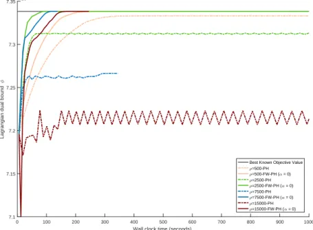
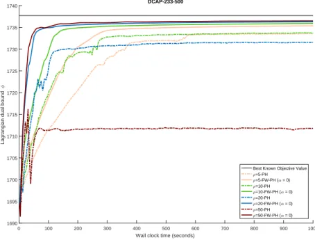
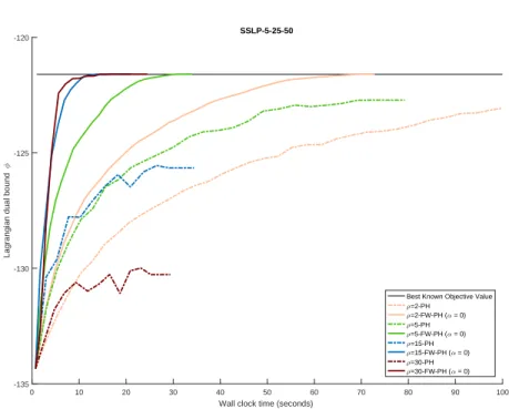
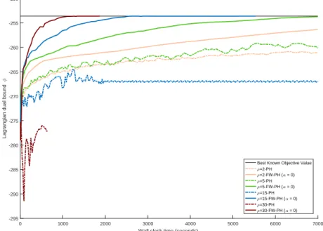
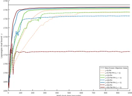
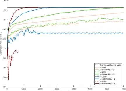
The FW-PH with α = 0 versus PH convergence profiles for the experiments performed are given in Figures 1–4, in which we provide plots of wall time versus Lagrangian bound values based on profiling of varying penalty for four of the eight problems considered. The times scales for the plots have been set such that trends are meaningfully depicted (1000s for CAP and DCAP instances, 100s for SSLP-5-25-50, and 7000s for SSLP-15-45-15). The trend of the Lagrangian bounds is depicted with solid lines for FW-PH withα= 0 and with dashed lines for PH. Plots providing the same comparison for FW-PH withα= 1 are provided in Appendix A.

As seen in the plots of Figures 1–4, the Lagrangian boundsφgenerated with PH tend to converge suboptimally, often displaying cycling, for large penalty values. In terms of the quality of the bounds obtained, while there is no clear winner when low penaltyρvalues are used, for large penalties, the quality of the boundsφgenerated with FW-PH is consistently better than for the bounds generated with PH, regardless of the αvalue. This last observation is significant because the effective use of large penalty valuesρin methods based on augmented Lagrangian relaxation tends to yield the most rapid early iteration improvement in the Lagrangian bound; this point is most clearly illustrated in the plot of Figure 3. The remaining plots have been omitted due to space limitations.

0 100 200 300 400 500 600 700 800 900 1000

Wall clock time (seconds)

7.1 7.15 7.2 7.25 7.3 7.35

Lagrangian dual bound

105 CAP-101-250

Best Known Objective Value =500-PH =500-FW-PH ( = 0) =2500-PH =2500-FW-PH ( = 0) =7500-PH =7500-FW-PH ( = 0) =15000-PH =15000-FW-PH ( = 0)

Fig. 1. Convergence profile for CAP-101-250 (PH and FW-PH withα= 0).

To assess the performance of the ideas discussed in section 3.2 concerning the generation of primal feasible solutions, we performed the following experiments. For PH, we used the solution of MIQPs (calculated in line 12 in Algorithm 1) returned by Algorithm 1 to give candidate first-stage solutions. Whenever PH has converged, a unique nonanticipative (first-stage) primal feasible integral solution is returned. Otherwise, PH might obtain distinct solutions for distinct scenarios; we evaluate all

(19)

0 100 200 300 400 500 600 700 800 900 1000

1690 1695 1700 1705 1710 1715 1720 1725 1730 1735 1740

DCAP-233-500

Fig. 2.Convergence profile for DCAP-233-500 (PH and FW-PH withα= 0).

Table 4

Result summary for CAP problem instances: primal bounds.

Gap (%) Time ρ PH H1 H2 PH H1 H2 20 0.00 0.00 0.00 130.26 984.17 288.24 100 0.00 0.00 0.00 3.74 102.43 13.90 500 0.00 0.00 0.00 8.26 6.32 9.09 1000 0.00 0.00 0.00 7.89 2.97 9.19 2500 0.00 0.00 0.00 19.42 5.44 12.02 5000 0.00 0.00 0.00 3.36 7.98 13.27 7500 0.00 0.00 0.00 3.29 2.64 8.28 15000 0.10 0.00 0.00 8.83 3.10 8.06

(a) CAP-101-250; absolute percentage gap based on the known optimal value733827.32.

(b) CAP-102-250; absolute percentage gap based on the known optimal value788996.97.

distinct solutions and report that with the best objective function value. For FW-PH, we analyze the two distinct strategies discussed in section 3, referred to as H1 and H2, respectively.

In Tables 4–6, the first column lists the values of the penalty parameterρwhile the remaining columns present for PH and FW-PH (for H1 and H2): (1) the absolute percentage gap between ζ∗ (i.e., either a known optimal value for the problem or a known best bound thereof) and the primal boundζ obtained as described, which is given by|(ζ−ζ∗)/ζ∗|, expressed as a percentage (column “Gap (%)”); and (2) the total wall clock time taken to evaluate all candidate solutions and select that with best objective function value. The results presented are for the variant of FW-PH consideringα= 0 only due to space limitations.

(20)

0 10 20 30 40 50 60 70 80 90 100

-135 -130 -125 -120

SSLP-5-25-50

Fig. 3.Convergence profile for SSLP-5-25-50 (PH and FW-PH withα= 0).

Table 5

Result summary for DCAP problem instances: primal bounds.

(a) DCAP-233-500; absolute percentage gap based on the best known upper bound1737.73.

(b) DCAP-243-500; absolute percentage gap based on the known optimal value2167.51.

As can be seen from these results, despite the simplicity of the proposed heuristics to obtain primal feasible solutions, in most cases the primal bounds generated are of good quality and often superior to those obtained from PH. Strategy H2 more often presents better performance when compared to H1, but with no clear winner between them in terms of percentage gap and time. The time taken for PH and FW-PH to evaluate the solutions is similar for the two methods, despite the heuristic used. One can notice that, in cases in which convergence is not observed (typically associated with the consideration of smaller penalty ρ), the time taken to evaluate solutions is typically higher due to the number of first-stage solutions to be considered. Overall, these results suggest that it is possible in practice to employ these heuristics as the times required are not prohibitive, particularly when convergence to a reasonably good dual bound has been observed.

(21)

0 1000 2000 3000 4000 5000 6000 7000

-295 -290 -285 -280 -275 -270 -265 -260 -255 -250

SSLP-15-45-15

Table 6

Result summary for SSLP problem instances: primal bounds.

Gap (%) Time ρ PH H1 H2 PH H1 H2 1 0.00 0.00 0.00 0.02 0.02 1.03 2 0.00 0.00 0.00 0.02 0.01 1.07 5 0.00 0.00 0.00 0.01 0.02 0.96 15 0.00 0.00 0.00 0.02 0.01 0.55 30 0.00 0.00 0.00 0.02 0.02 0.36 50 0.00 0.00 0.00 0.01 0.02 0.18 100 2.15 0.00 0.00 0.02 0.02 0.08

(a) SSLP-5-25-50; absolute percentage gap based on the known optimal value−121.60.

(b) SSLP-5-25-100; absolute percentage gap based on the known optimal value−127.37.

(c)SSLP-10-50-100; absolute percentage gap based on the known optimal value−354.19.

(d) SSLP-15-45-15; absolute percentage gap based on the known optimal value−253.60.

(22)

5. Conclusions and future work. In this paper, we have presented an alter-native approach to computing nonanticipativity Lagrangian bounds associated with SMIPs that combines ideas from the progressive hedging (PH) and the Frank–Wolfe (FW) methods. We first note that while Lagrangian bounds can be recovered with PH, this requires—for each iteration and each scenario—the solution of an additional MILP subproblem in addition to the MIQP subproblem. Furthermore, when using the PH method directly, the Lagrangian bounds may converge suboptimally, cycle (for large penalties), or converge very slowly (for small penalties).

To overcome the lack of theoretical support for the above use of PH, we first described a straightforward integration of PH and an FW-like approach such as the simplicial decomposition method (SDM), where SDM is used to compute the primal updates in PH. Its convergence only requires noting that SDM applied to a convex problem with a bounded polyhedral constraint set terminates finitely with optimal convergence. However, for the stated goal of computing high-quality Lagrangian bounds efficiently, the benefits of relying on the optimal convergence of SDM is far outweighed by the computational costs incurred.

As an alternative, we propose the contributed algorithm, FW-PH, that is ana-lyzed under general assumptions on how the Lagrangian bounds are computed and on the number of SDM iterations used for each dual update. Furthermore, under mild assumptions on the initialization of the algorithm, FW-PH only requires the so-lution of a MILP subproblem and a continuous convex quadratic subproblem for each iteration and each scenario. FW-PH is versatile enough to handle a wide range of SMIPs with integrality restrictions in any stage, while providing rapid improvement in the Lagrangian bound in the early iterations that is consistent across a wide range of penalty parameter values. Although we have opted to focus on two-stage problems with recourse, the generalization of the proposed approach to the multi-stage case is also possible.

The numerical results are encouraging as they suggest that the proposed FW-PH method applied to SMIP problems usually outperforms the traditional PH method with respect to how quickly the quality of the generated Lagrangian bounds improves. This is especially true with the use of larger penalty values. For all problems consid-ered and for all but the smallest penalties considconsid-ered, the FW-PH method displayed better performance over PH in terms of the quality of the final Lagrangian bounds at the end of the allotted wall clock time.

The improved performance of FW-PH over PH for large penalties is significant because it is the effective use of large penalties enabled by FW-PH that yields the most rapid initial dual improvement. This last feature of FW-PH would be most help-ful in its use within a branch-and-bound or branch-and-cut framework for providing strong lower bounds (in the case of minimization). In addition to being another means to compute Lagrangian bounds, PH would still have a role in such frameworks as a heuristic for computing a primal feasible solution to the SMIP, thus providing (in the case of minimization) an upper bound on the optimal value. In fact, as demonstrated by our numerical experiments, straightforward combinations of both methods pro-vide heuristics that are capable of generating very good primal feasible solutions for the problems considered. This suggests that the development of more sophisticated heuristics is also a promising avenue of research.

Possible directions for future research include the following. First, FW-PH inher-its the potential for parallelization from PH. Experiments for exploring the benefit of parallelization are therefore warranted. Second, the theoretical support of FW-PH can be strengthened with a better understanding of the behavior of PH (and its

(23)

eralization ADMM) applied to infeasible problems. Finally, FW-PH can benefit from a better understanding of how the proximal term penalty coefficient can be varied to improve performance.

Appendix A. Additional plots for PH vs. FW-PH for α= 1.

0 100 200 300 400 500 600 700 800 900 1000

7.1 7.15 7.2 7.25 7.3 7.35

105 CAP-101-250

Fig. 5. Convergence profile for CAP-101-250 (PH and FW-PH withα= 1).

0 100 200 300 400 500 600 700 800 900 1000

1690 1695 1700 1705 1710 1715 1720 1725 1730 1735 1740

DCAP-233-500

Fig. 6.Convergence profile for DCAP-233-500 (PH and FW-PH withα= 1).

(24)

0 10 20 30 40 50 60 70 80 90 100

-135 -130 -125 -120

SSLP-5-25-50

0 1000 2000 3000 4000 5000 6000 7000

-295 -290 -285 -280 -275 -270 -265 -260 -255 -250

SSLP-15-45-15

(25)

REFERENCES [1] http://www.nci.org.au. Last accessed 20 April, 2016.

[2] http://www2.isye.gatech.edu/∼_{sahmed/siplib/sslp/sslp.html.} _{Last accessed 23 December,}

2015.

[3] COmputational INfrastructure for Operations Research, http://www.coin-or.org/. Last ac-cessed 28 January, 2016.

[4] A. Agust´ın, A. Alonso-Ayuso, L. F. Escudero, and C. Pizarro,On air traffic flow man-agement with rerouting. Part II: Stochastic case, European J. Oper. Res., 219 (2012), pp. 167–177.

[5] S. Ahmed and R. Garcia,Dynamic capacity acquisition and assignment under uncertainty, Ann. Oper. Res., 124 (2003), pp. 267–283.

[6] F. Badilla Veliz, J.-P. Watson, A. Weintraub, R. J.-B. Wets, and D. L. Woodruff,

Stochastic optimization models in forest planning: A progressive hedging solution approach, Ann. Oper. Res., 232 (2015), pp. 259–274.

[7] M. Bodur, S. Dash, O. G¨unl¨uk, and J. Luedtke,Strengthened Benders Cuts for Stochastic Integer Programs with Continuous Recourse, preprint, http://www.optimization-online. org/DB FILE/2014/03/4263.pdf, 2014.

[8] S. Boyd, N. Parikh, E. Chu, B. Peleato, and J. Eckstein,Distributed Optimization and Statistical Learning via the Alternating Direction Method of Multipliers, Foundations and Trends in Machine Learning, Vol. 3, Issue 1, Now Publishers, Hanover, MA, 2011, http: //dx.doi.org/10.1561/2200000016.

[9] C. C. Carøe and R. Schultz,Dual decomposition in stochastic integer programming, Oper. Res. Lett., 24 (1999), pp. 37–45.

[10] J. Chen, C. H. Lim, P. Qian, J. Linderoth, and S. J. Wright,Validating Sample Average Approximation Solutions with Negatively Dependent Batches, preprint, http://arxiv.org/ abs/1404.7208, 2014.

[11] T. H. de Mello,On rates of convergence for stochastic optimization problems under non-independent and identically distributed sampling, SIAM J. Optim., 19 (2008), pp. 524–551. [12] J. Eckstein and D. Bertsekas,On the Douglas–Rachford splitting method and the proximal point algorithm for maximal monotone operators, Math. Program., 55 (1992), pp. 293–318. [13] M. Frank and P. Wolfe,An algorithm for quadratic programming, Naval Res. Logist. Quart.,

3 (1956), pp. 149–154.

[14] D. Gabay and B. Mercier,A dual algorithm for the solution of nonlinear variational problems via finite element approximation, Comput. Math. Appl., 2 (1976), pp. 17–40.

[15] D. Gade, G. Hackebeil, S. M. Ryan, J.-P. Watson, R. J.-B. Wets, and D. L. Woodruff,

Obtaining lower bounds from the progressive hedging algorithm for stochastic mixed-integer programs, Math. Program., 157 (2016), pp. 47–67.

[16] M. R. Hestenes,Multiplier and gradient methods, J. Optim. Theory Appl., (1969), pp. 303– 320.

[17] C. Holloway, An extension of the Frank and Wolfe method of feasible directions, Math. Program., 6 (1974), pp. 14–27.

[18] IBM Corporation, IBM ILOG CPLEX V12.5; available at http://www-01.ibm.com/soft

ware/commerce/optimization/cplex-optimizer/. Last accessed 28 Jan 2016.

[19] A. Kleywegt, A. Shapiro, and T. Homem-de-Mello,The sample average approximation method for stochastic discrete optimization, SIAM J. Optim., 12 (2001), pp. 479–502. [20] G. Laporte, F. V. Louveaux, and H. Mercure,The vehicle routing problem with stochastic

travel times, Transp. Sci., 26 (1992), pp. 161–170.

[21] A. Løkketangen and D. Woodruff,Progressive hedging and tabu search applied to mixed integer (0,1) multi-stage stochastic programming, J. Heuristics, 2 (1996), pp. 111–128. [22] F. V. Louveaux,Discrete stochastic location models, Ann. Oper. Res., 6 (1986), pp. 23–34. [23] M. Lubin, K. Martin, C. Petra, and B. Sandıkc¸ı,On parallelizing dual decomposition in

stochastic integer programming, Oper. Res. Lett., 41 (2013), pp. 252–258.

[24] W. K. Mak, D. P. Morton, and R. K. Wood,Monte Carlo bounding techniques for deter-mining solution quality in stochastic programs, Oper. Res. Lett., 24 (1999), pp. 47–56. [25] G. Nemhauser and L. Wolsey,Integer and combinatorial optimization, Wiley-Intersci. Ser.

Discrete Math. Optim., Wiley-Interscience, New York, 1988.

[26] M. P. Nowak and W. R¨omisch,Stochastic Lagrangian relaxation applied to power scheduling

in a hydro-thermal system under uncertainty, Ann. Oper. Res., 100 (2000), pp. 251–272. [27] L. Ntaimo,Decomposition Algorithms for Stochastic Combinatorial Optimization:

Computa-tional Experiments and Extensions, Ph.D. thesis, University of Arizona, AZ, 2004. [28] L. Ntaimo, J. A. G. Arrubla, C. Stripling, J. Young, and T. Spencer, A stochastic

(26)

programming standard response model for wildfire initial attack planning, Can. J. For. Res., 42 (2012), pp. 987–1001.

[29] L. Ntaimo and S. Sen,The million-variable “march” for stochastic combinatorial

optimiza-tion, J. Global Optim., 32, pp. 385–400.

[30] O. Y. ¨Ozaltın, O. A. Prokopyev, A. J. Schaefer, and M. S. Roberts, Optimizing the societal benefits of the annual influenza vaccine: A stochastic programming approach, Oper. Res., 59 (2011), pp. 1131–1143.

[31] M. J. D. Powell,A method for nonlinear constraints in minimization problems, in Optimiza-tion, R. Fletcher, ed., Academic Press, New York, 1969.

[32] R. T. Rockafellar and R. J.-B. Wets,Scenarios and policy aggregation in optimization under uncertainty, Math. Oper. Res., 16 (1991), pp. 119–147.

[33] A. Ruszczy´nski,Nonlinear Optimization, Princeton University Press, Princeton, NJ, 2006.

[34] J. Salmeron, R. K. Wood, and D. P. Morton,A stochastic program for optimizing military sealift subject to attack, Military Oper. Res., 14 (2009), pp. 19–39.

[35] N. Shor,Minimization Methods for Non-Differentiable Functions, Springer-Verlag, New York, 1985.

[36] S. Takriti, J. Birge, and E. Long,A stochastic model for the unit commitment problem, IEEE Trans. Power Syst., 11 (1996), pp. 1497–1508.

[37] M. W. Tanner, L. Sattenspiel, and L. Ntaimo,Finding optimal vaccination strategies under parameter uncertainty using stochastic programming, Math. Biosci., 215 (2008), pp. 144– 151.

[38] B. Von Hohenbalken,Simplicial decomposition in nonlinear programming algorithms, Math. Program., 13 (1977), pp. 49–68.

[39] J. Watson and D. Woodruff,Progressive hedging innovations for a class of stochastic re-source allocation problems, Comput. Manag. Sci., 8 (2011), pp. 355–370.