WAVELETS FOR SELF-CALIBRATED BUNDLE BLOCK ADJUSTMENT
Jun-Fu Ye 1, *, Jaan-Rong Tsay 21 Dept. of Geomatics, National Cheng Kung University, Taiwan - [email protected] 2 Dept. of Geomatics, National Cheng Kung University, Taiwan - [email protected]
KEY WORDS: bundle block adjustment, additional parameters, wavelets, function approximation, image distortion, photogrammetry, self-calibration
ABSTRACT:
This paper entails a methodological novelty and builds upon prior research on a wavelets-based model for digital camera self-calibration. We introduce a new kernel function based on the compactly supported orthogonal third-order asymmetric Daubechies wavelet to correct systematic image distortion errors. Tests are done by using aerial images taken with a high-resolution metric digital aerial mapping camera. The quality of experimental results is evaluated by using reliable and high precision ground check points in the calibration field. For example, a four-fold block with this wavelet self-calibration model has the external accuracy of about 0.28 GSD (=ground sampling distance) in the horizontal direction, and about 0.43 GSD in the vertical direction, respectively, where 1GSD 4.6cm. The posterior standard deviations of unit weight are reduced from 0.37 pixel to 0.27 pixel. The residual vector lengths are also significantly reduced after our wavelet additional parameters are used. Experimental results support the proposal and demonstrate the applicability of this new model.
1. INTRODUCTION
Digital images are widely used to record geometric, radiometric and semantic information in a target scene of interest. However, digital image has inevitably defects caused by some external factors, such as deviations in the manufacture and parts assembly of camera components, resulting in systematic differences between both actual and theoretical projections during the imaging process. Therefore, in the fields of photogrammetry, geometric computer vision, or optical engineering, high-precision geometric applications must take the effects of these systematic errors into account. A technique of determining the interior orientation parameters (IOPs) of cameras is called “camera calibration”. These IOPs include principal distance c (or focal length) of camera, the photo coordinates of the principal point (x0, y0), and lens distortion parameters. Camera self-calibration technique is commonly the most widely used method in photogrammetry, and has the ability to automatically select the appropriate additional parameters (APs) by means of statistical tests to correct the camera lens distortion.
Many early studies proposed different traditional APs based on mathematics or physical phenomena to describe the lens distortion of analogue cameras. For example, the most classic physical self-calibration model was firstly proposed by Brown (1971) for calibrating the lens distortion of close-range cameras, and then Brown (1976) extended his model to calibrate the lens distortion of single-head analogue aerial cameras. Some traditional mathematical self-calibration models, such as those proposed by Ebner (1976), El-Hakim & Faig (1977), and Grün (1978), were established by using algebraic polynomials and spherical harmonics as mathematical basis functions. Although these traditional self-calibration models are helpful to improve the external accuracy of photo triangulation, Clarke and Fryer (1998) reveals that many of the traditional APs lack the foundations for observable physical phenomena and have the risks of over-parameterization and high correlation with other correction parameters. In the era of digital photogrammetry, these traditional self-calibration models are also continuously used to calibrate diverse modern new types of digital aerial cameras although they might not be suitable for accurately calibrating the lens distortion
of different kinds of digital cameras (Fritsch, 2015). Cramer (2009) and Jacobsen et al. (2010) calibrated a variety of digital aerial cameras with different self-calibration models to correct lens distortion of these cameras and verify their results. However, some of aforementioned inherent defects of traditional APs still exist.
Tang et al. (2012a) proposed a series of Legendre self-calibration APs based on orthogonal univariate Legendre polynomials to calibrate the lens distortion of digital aerial frame cameras. The correlations of Legendre self-calibration APs are lower than those of the traditional self-calibration APs, but an inherent defect of all polynomial APs, which is not completely independent between the x and y components of camera lens distortion, still exists. Tang (2012b) used bivariate Fourier series to define a family of Fourier self-calibration APs, which overcomes the drawback of all polynomial APs and has the advantages of orthogonal, mathematically rigorous, flexible, generic and efficient calibration of the lens distortion of all digital aerial frame cameras. Fourier is most suitable for representing and analyzing stationary signals, but it has inherent defects in displaying and decomposing non-stationary signals. Briefly to say, stationary image distortion signals are constant in their statistical parameters over the whole image array. Their frequency contents do not change from place to place in an image. However, the lens distortion signals of diverse modern new types of digital cameras might be stationary partly and non-stationary another partly. In order to implement the novel ideas and to explore the possible application potential of wavelets on self-calibrating distortion parameters of modern diverse types of digital cameras, the orthogonal wavelet functions are adopted and used as the mathematical basis functions to establish new camera self-calibration APs, called wavelet APs (WAPs), in our studies since 2016. The WAPs have similar advantages as Fourier APs such as mathematical rigorousness, orthogonality between any two wavelet (child) functions, model flexibility, generic applicability and computation efficiency for camera self-calibration. Moreover, some wavelets such as both asymmetric and least asymmetric families of Daubechies wavelets still have advantages in expressing both stationary and The International Archives of the Photogrammetry, Remote Sensing and Spatial Information Sciences, Volume XLIII-B1-2020, 2020
non-stationary, or even fractal distortion signals of digital images.
Section 2 summarizes briefly the fundamental theory and concepts of wavelets as well as the related wavelet issues used in the current WAP model. And section 3 describes our WAP model briefly. In section 4, both introduction to our tests by using real digital aerial images and their test results are given. The performance of WAPs is evaluated, too. Some conclusions are then drawn in section 5.
2. BRIEF INTRODUCTION TO THE RELATED
WAVELET ISSUES
Briefly speaking, wavelet theory and wavelet functions as well provide the second generation tool for signal and image processing, whereas the well-known Fourier theory and its kernel functions, namely sinusoidal and cosine functions in different frequency bands, as well give the first generation tool for signal and image processing. They include the wavelet series, continuous wavelet transform (CWT), discrete wavelet transform (DWT), fast wavelet transform (FWT) in the wavelet tools, as well as the Fourier series, continuous Fourier transform (CFT), discrete Fourier transform (DFT), fast Fourier transform (FFT) in the Fourier tools, respectively. Generally speaking, wavelets suit for representation and processing of both non-stationary and non-stationary signals, while the Fourier tools are good only for stationary signals.
Stationary signals are constant in their statistical parameters over time. If you look at a stationary signal for a few moments and then wait an hour and look at it again, it would look essentially the same, i.e. its overall level would be about the same and its amplitude distribution and standard deviation would be also about the same. On the other hand, signals whose frequency contents do not change over time are called stationary signals. In other words, the frequency content of stationary signals does not change over time. In this case, one does not need to know at what time durations frequency components exist, since all frequency components exist at all time locations. The sine and cosine functions are two typical examples of stationary signal functions.
Contrary to the aforementioned examples of stationary signals, those signals, whose frequency constantly changes over time, are known as non-stationary ones. For instance, the "chirp" signal is non-stationary.
Mallat (1989) proposed a theory for multiresolution signal decomposition. Multi-resolution analysis (MRA) plays an important role in the wavelet theory, and is often called multi-scale analysis (MSA), too. It enables an efficient both signal, including image, decomposition and reconstruction in different levels of details. The wavelet representation can be used to display signals inclusive of two-dimensional image distortion functions.
For the present, there are already diverse kinds of digital cameras such as digital frame cameras, virtual image composition cameras, multi-head cameras, fish-eye cameras, push-broom cameras, linear array cameras and so on. They may be metric or non-metric. The inherent image distortion may be stationary or non-stationary. Wavelets are able to represent both stationary and non-stationary image distortion signals.
apparently the correct mathematics for describing image texture (Jaehne, 1991) and real signals in nature. Real signals in nature are often fractal or Hoelder-continuous (also called “lipschitz continuous”) (Daubechies, 1994; Kaiser, 1994; Louis et al., 1994). They are often not able to be described by traditional analytical functions or, briefly to say, to be expressed in a closed form. These signals in nature often have varied degrees of continuity from place to place. On the other hand, many signals in nature are fractal, and have the properties of, e.g., self-similarity or self-affinity. Due to the aforementioned considerations, wavelets are selected and applied in this study to design a new model called WAP, which is expected to be able to self-calibrate diverse kinds of digital cameras.
Tsay (2016) proposed some original ideas for designing the WAP models, and mentioned that not only the theoretical and practical wavelet series (Strang, Nguyen, 1996) but also both the S-D model for interpolation and S-model for approximation proposed by Tsay (1996) can be extended and utilized for designing the WAP models. In this study, one of those novel models for WAP is proposed and tested. The concerned computation algorithm and the corresponding program system for self-calibrated bundle block adjustment are also developed by using the program language C# on a general personal computer.
Furthermore, there are already diverse kinds of wavelet functions which might be available for this WAP model, such as Haar wavelets, Daubechies wavelets, Littlewood-Paley wavelet, Morlet wavelet, Meyer wavelet, Battle-Lemarie wavelets. They might be biorthogonal, orthogonal, semi-orthogonal, or non-orthogonal wavelets. On the other hand, they might be compactly supported or not compactly supported. They might be real or complex wavelets. They may be continuous or discontinuous. Their function curves may be smooth or not smooth. These diverse wavelet functions may be regular or irregular. Their function curves might be symmetric or asymmetric. Some of them can be displayed explicitly, but the others cannot be described in a closed-form expression. Anyway, the accuracy, rigorousness and flexibility of this approximation model for image distortion and the computation complexity, namely the number of addition and multiplication operations, are taken into account in this study for selecting a proper wavelet family for our WAP model. For the present, the orthogonal, compactly supported asymmetric Daubechies wavelets of third order (N=3) including their father wavelet and scaled and translated scaling functions jk, j,kZ, are adopted in this study for establishing the WAP model, where the symbol Z denotes the set of all integers.
Moreover, the orthogonal, compactly supported asymmetric Daubechies wavelets of third order (N=3) cannot be displayed explicitly in a closed-form expression. Nevertheless, their function values can be computed as accurately as needed by means of different methods such as Cascade Algorithm (Daubechies, Lagarias, 1991), Strang’s method (Strang, 1989), Fourier algorithm (Daubechies, 1994), and Kaiser’s Method of Cumulants (Kaiser, 1994). Moreover, Tsay (1996) proposed a method for calculating the derivative functions of Daubechies wavelets for the order N3, where a linearly independent equation given by Dahmen and Micchelli (1990) is applied for solving the rank defect problem in a linear equation system. The International Archives of the Photogrammetry, Remote Sensing and Spatial Information Sciences, Volume XLIII-B1-2020, 2020
The self-calibration models can be incorporated into the well-known collinearity condition equations in photogrammetry (Wolf and Dewitt, 2000), as shown in (1).
∆ ∆
1
where x and y are photo coordinates of an image point of interest; X, Y, and Z are the object coordinates of its corresponding object point; c is the camera focal length; x0 and y0 are the photo coordinates of the principal point; X0, Y0, and Z0 are the object coordinates of camera exposure station; r’s are the functions of three rotation angles, e.g. omega , phi , and kappa ; ∆x and ∆y are the systematic error components in the photo coordinates x and y, respectively; εx and εy are the random
error components in the photo coordinate observations x and y, respectively.
We develop novel self-calibration additional parameters based on orthogonal wavelet functions, which are used to calibrate the digital frame cameras in the Cartesian coordinate system of Euclidean space. The systematic error components ∆x and ∆y in (1) can be given as (2), where W and H are the width and height of image, respectively; sx and sy are the scale factors of the wavelet basis functions in the x and y directions, respectively; aij and bij are the coefficients of WAPs in ∆x and ∆y, respectively; i and j are the translation parameters of the wavelet basis functions in the x and y directions, respectively; is Daubechies father wavelet function ϕ of order N defined in (3), where hn, ∀n, are the low-pass filter coefficients (Daubechies,
1994).
∆ ∆ , , , , , , ,
∆ ∆ , , , , , , , 2 √2 2 3
The total number of WAP coefficients is determined by the definition of all parameters in Eq. (2). The number of significant WAPs used is decided automatically by the statistical tests, including correlation test, significance test and total correlation test. The thresholds for these statistical tests are referenced from the empirical values of the classic bundle adjustment software BINGO (Kruck, 2016).
4. SELF-CALIBRATION TESTS AND EVALUATION
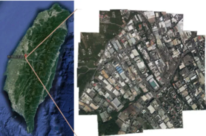
The WAPs are tested in a test area located in Nangang, Nantou County, Taiwan. The test area shown in Figure 1 is an aerial camera calibration field built by the National Land Surveying and Mapping Center, Ministry of the Interior, Taiwan. A total of 30 test images with 80% end lap and 60% side lap are taken with an UltraCam Xp Wide Angle digital aerial camera, and they are composed of three east-west and three north-south flight strips, each of which has 5 test images. The parameters of these test images are shown in Table 1.
Figure 1. Location of the test area in Taiwan and its image coverage
Acquisition Date September 21, 2012
Camera UltraCam Xp Wide Angle
Focal Length 70.500 ± 0.002 mm
Pixel Size 6.0 μm
Image Size 11310 pixels × 17310 pixels
End lap ≈ 80%
Side lap ≈ 60%
Height (AGL) ≈ 545 m
Groundel Size ≈ 46 mm
Image Scale ≈ 1:7700
Calibration Field Size 750 m × 600 m Ground Coverage ≈ 1433 m × 1433 m
Table 1. The parameters of the test images
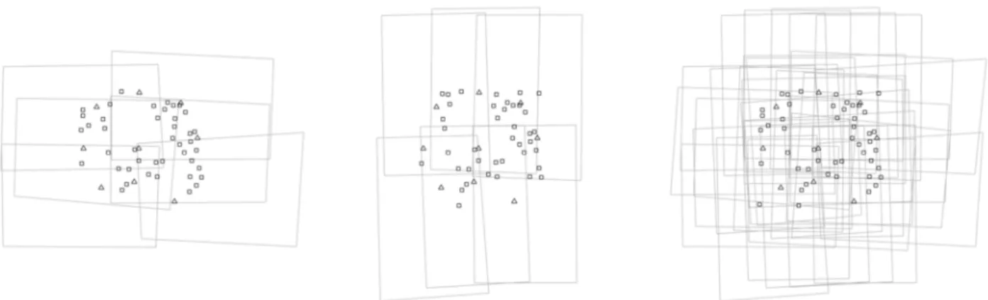
Three sets of test images are tested, including (case 1) a block composed of two north-south flight strips with 60% end lap and 25% side lap, (case 2) a block composed of two east-west flight strips with 60% end lap and 25% side lap, and (case 3) a block composed of cross strips with 80% end lap and 60% side lap. Each set of test images is used in both test cases of the bundle block adjustments without WAPs and with WAPs, respectively. The case number and the number of known ground points (GCPs and CHKs) are shown in Table 2, where the number of check points (CHKs) is 42 (case 1), 41 (case 2) and 49 (case 3), respectively, due to different image coverage in these three test cases. The distribution maps of all used known points and the image overlap of all used images are shown in Figure 2, where triangles and squares denote the full ground control points (GCPs) and the full check points (CHKs), respectively. Figure 2 shows that all known ground target points including GCPs and CHKs are located inside the image coverage. There is not any known ground target point on the border and corners of the block model. This is evidently a defect of this study.
Without WAPs With WAPs North-south flight strips
(9GCPs / 42CHKs) Case 1-1 Case 1-2
East-west flight strips
(9GCPs / 41CHKs) Case 2-1 Case 2-2
Cross flight strips
(9GCPs / 49CHKs) Case 3-1 Case 3-2
Table 2. Test cases
The International Archives of the Photogrammetry, Remote Sensing and Spatial Information Sciences, Volume XLIII-B1-2020, 2020 XXIV ISPRS Congress (2020 edition)
Figure 2. The distribution maps of all used known points, where triangles and squares denote the full GCPs and the full CHKs, respectively, and the image overlap of all used images in Case 1 (left), Case 2 (middle), and Case 3 (right)
The observations include the photo coordinates of all tie points and the object coordinates of all ground control points (GCPs). The unknown parameters include the wavelet additional parameters (WAPs) in the cases 1-2, 2-2 and 3-2, the exterior orientation parameters of all test images used, and the ground coordinates of all object points. All image points on all used images are overlaid in the image frame as shown in Figure 3, which illustrates that the average image point density is 0.28 points/mm2 (case 1), 0.29 points/mm2 (case 2) and 2.02 points/mm2, respectively. Apparently, the case 3 has significantly larger point density than the cases 1 and 2. The bundle block adjustment results of all test cases are summarized in Table 3. By using the statistical tests mentioned in Section 3, the number of significant WAPs is reduced from 234 to 52 (about 22% of all original WAPs in the wavelet model) for the two cases 1-2 and 2-2 of single block with WAPs, and reduced from 234 to 106 (about 45% of all WAPs) for the case 3-2 of four-fold block with WAPs. After using WAPs for self-calibration, the posterior standard deviations of unit weight in the three sets of test cases are significantly reduced from 0.33 pixel to 0.27 pixel in the case 1, from 0.28 pixel to 0.23 pixel in the case 2, and from 0.37 pixel to 0.27 pixel in the case 3. The average redundancy is (n-u)/n, where n and u denote the number of observations and unknowns, respectively. Table 3 demonstrates apparently that the average redundancy in the case 3 is about 0.80 which is larger significantly than 0.32~0.36 in the cases 1 and 2. Also, the case 3 spends 15~85 seconds for computations which is much longer that <1~4 seconds in the cases 1 and 2.
Figure 3. Overlaying all image points of all used images in the image frame
Case Number of WAPs px redundancy Average Calculation Time
1-1 - 0.33 0.36 < 1 s 1-2 52/234 0.27 0.34 2 s 2-1 - 0.28 0.33 < 1 s 2-2 52/234 0.23 0.32 4 s 3-1 - 0.37 0.80 15 s 3-2 106/234 0.27 0.79 85 s
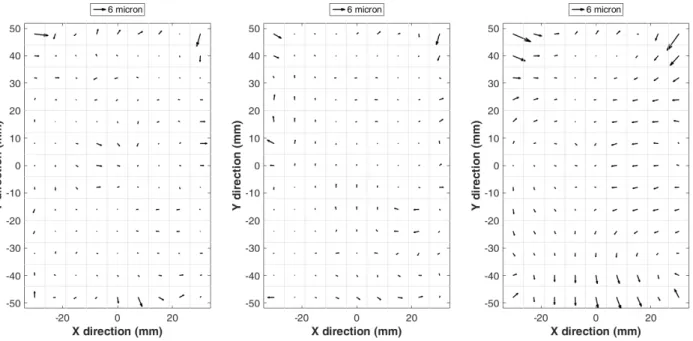
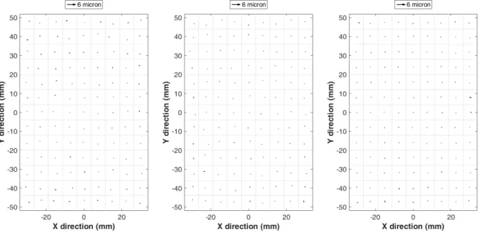
Table 3. The bundle block adjustment results of all test cases Figure 4 illustrates the average image distortion vectors estimated by the WAP model on all 0.1mm × 0.1mm grid points in a tile in the cases 1-2, 2-2 and 3-2 with WAPs, where an image frame is divided into 9 × 13 tiles. The average image distortion vectors calculated by the three sets of test images are different because they have different number and distribution of the tie points. For these three cases, the number of the tie points in a tile is in the range [4, 33], [7, 33], and [52, 172], respectively. Therefore, the average image distortion vectors of Case 1-2 and Case 2-2 are not considered to be significant. Moreover, the average residual vectors of all photo coordinate observations in the cases of “without WAPs” and “with WAPs” are displayed in Figure 5 and Figure 6, respectively. They illustrate that the average residual vectors of the photo coordinate observations have no significant systematic errors, and these residual vector lengths are also significantly reduced after WAPs are used. These test results indicate that this wavelet model for self-calibrated bundle block adjustment is helpful and applicable to correct the systematic distortion errors of images taken with aerial digital mapping cameras.
The International Archives of the Photogrammetry, Remote Sensing and Spatial Information Sciences, Volume XLIII-B1-2020, 2020 XXIV ISPRS Congress (2020 edition)
Figure 4. Average image distortion vectors determined by using WAPs in Case 1-2 (left), Case 2-2 (middle), and Case 3-2 (right)
Figure 5. Average residual vectors of the photo coordinate observations in Case 1-1 (left), Case 2-1 (middle), and Case 3-1 (right) The International Archives of the Photogrammetry, Remote Sensing and Spatial Information Sciences, Volume XLIII-B1-2020, 2020
Figure 6. Average residual vectors of the photo coordinate observations in Case 1-2 (left), Case 2-2 (middle), and Case 3-2 (right)
Figure 7. The horizontal coordinate difference vectors (left) and elevation difference vectors (right) on all CHKs The International Archives of the Photogrammetry, Remote Sensing and Spatial Information Sciences, Volume XLIII-B1-2020, 2020
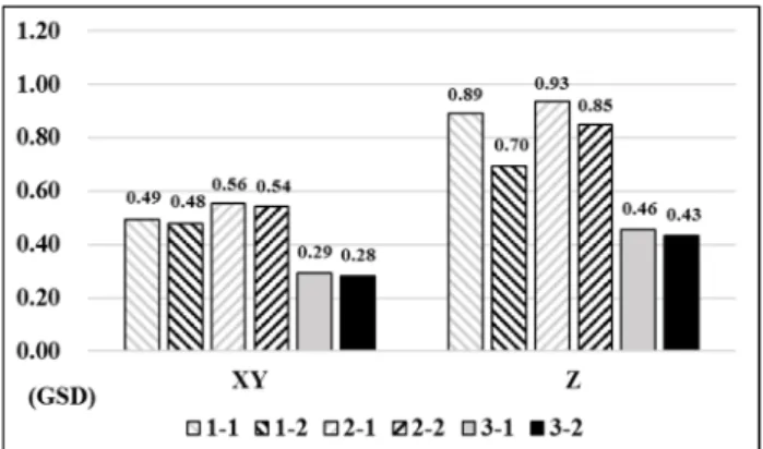
The external accuracy of all test cases shown in Figure 8 is derived from the root mean square discrepancies of all independent ground check points (CHKs) used. The object coordinates of all known points, including GCPs and CHKs, are measured by static GNSS surveying, whose accuracy is sufficient to evaluate the results of aerial triangulation. For the two cases of single block without self-calibration, the external accuracy is about 0.49 GSD and 0.56 GSD in the horizontal direction, and about 0.89 GSD and 0.93 GSD in the vertical direction, respectively, where 1 GSD 4.6 cm. However, in these two cases with WAPs, the external accuracy is improved to about 0.48 GSD and 0.54 GSD in the horizontal direction, and to about 0.70 GSD and 0.85 GSD in the vertical direction, respectively. For the case of four-fold block, high image overlaps and side laps as well as cross strips do help to eliminate some systematic errors and increase the average redundancy. The external accuracy in the case of “without WAPs” and “with WAPs” is about 0.29 GSD and 0.28 GSD in the horizontal direction, and about 0.46 GSD and 0.43 GSD in the vertical direction, respectively. Figure 7 illustrates the ground coordinate difference vectors on all CHKs in the horizontal and elevation directions in each case.
Figure 8. External accuracy of all test cases
The root mean square (RMS) values of the posterior accuracies
, of all ground points in all test cases are illustrated in Figure 9. For the cases of “without WAPs”, the RMS values of
, are about 0.40 GSD, 0.39 GSD, and 0.58 GSD in the horizontal direction, and about 0.87 GSD, 0.80 GSD, and 1.02 GSD in the vertical direction, respectively. Nevertheless, for the cases of “with WAPs”, the RMS values of , are about 0.36 GSD, 0.31 GSD, and 0.43 GSD in the horizontal direction, and about 0.72 GSD, 0.65 GSD, and 0.76 GSD in the vertical direction, respectively.
Figure 9. The RMS of , of all ground points
The RMS values of the posterior accuracies , of all GCPs used in all test cases are illustrated in Figure 10. For the cases of “without WAPs”, the RMS values of , are about 0.12 GSD, 0.12 GSD, and 0.06 GSD in the horizontal direction, and about 0.20 GSD, 0.17 GSD, and 0.09 GSD in the vertical direction, respectively. Nevertheless, for the cases of “with WAPs”, the RMS values of , are about 0.11 GSD, 0.09 GSD, and 0.06 GSD in the horizontal direction, and about 0.17 GSD, 0.15 GSD, and 0.07 GSD in the vertical direction, respectively.
Figure 10. The RMS of , of all GCPs used
5. CONCLUSIONS
We develop novel wavelet additional parameters (WAPs) for self-calibrating digital frame cameras in the Cartesian coordinate system of Euclidean space. The test cases use aerial images taken with an UltraCam Xp Wide Angle digital aerial camera to perform bundle block adjustment without or with WAPs. For the two cases of single block with this wavelet self-calibration model, the external accuracy is about 0.48 to 0.54 GSD in the horizontal direction, and about 0.70 to 0.85 GSD in the vertical direction, respectively. For the case of four-fold block with this wavelet self-calibration model, the external accuracy is about 0.28 GSD in the horizontal direction, and about 0.43 GSD in the vertical direction, respectively. In addition, the number and distribution of the tie points may affect the solution of WAPs. These test results indicate that this wavelet model for self-calibrated bundle block adjustment is helpful and applicable to correct the systematic distortion errors of images taken with aerial digital mapping cameras by choosing a sufficient number and proper distribution of the tie points. Its applications for self-calibrating other digital cameras such as fisheye cameras will be further studied.
6. ACKNOWLEDGEMENTS
We sincerely appreciate the Ministry of Science and Technology (MOST), Taiwan, for the financial supports to our research projects for four years so far with the research grants MOST 105-2119-M-006-032, MOST 106-2119-M-006-023, MOST 107-2119-M-006-019 and MOST 108-2621-M-006-002. Also, we truly appreciate the GeoForce Technologies Co., Ltd, Taipei, Taiwan, for providing the aerial images taken with UltraCam Xp Wide Angle digital aerial camera over the calibration field for testing our wavelet model for camera self-calibration. Moreover, best thanks must be expressed to the National Land Surveying and Mapping Center (NLSC), Ministry of the Interior (MOI), Taiwan, for providing the ground target point data in the calibration field. Finally, we would like to express our sincere thanks to the blind reviewers of ISPRS 2020 for their valuable comments to this paper. The International Archives of the Photogrammetry, Remote Sensing and Spatial Information Sciences, Volume XLIII-B1-2020, 2020
REFERENCES
Brown, D., 1971. Close-range camera calibration. Photogrammetric Engineering, 37(8), 855-866.
Brown, D., 1976. The bundle method – progress and prospects. International Archives of Photogrammetry 21 (Part 3), 1-33. Clarke, T., Fryer, J., 1998. The development of camera calibration methods and models. Photogrammetric Record, 16(91), 51-66.
Cramer, M., (Ed.), 2009. Digital Camera Calibration. EuroSDR official publication No. 55.
Dahmen, W., Micchelli, C.A., 1990. Using the Refinement Equation for Evaluating Integrals of Wavelets. Fachbereich Mathematik, Serie A, Mathematik, Frei Universitaet Berlin, Preprint No. A-91-14.
Daubechies, I., Lagarias, J., 1991. Two-scale difference equations I. Existence and global regularity of solutions. Society for Industrial and Applied Mathematics (SIAM) Journal on Mathematical Analysis, 22, 1388-1410.
Daubechies, I., 1994. Ten Lectures on Wavelets. Society for Industrial and Applied Mathematics Philadelphia, PA, USA. Ebner, H., 1976. Self-calibrating block adjustment. Bildmessung und Luftbildwesen, 44(4), 128-139.
El-Hakim, S., Faig, W., 1977. Compensation of systematic image errors using spherical harmonics. Proceedings of the American Society of Photogrammetry, Fall technical meeting, Little Rock, Arkansas, 492-499.
Fritsch, D., 2015. Some Stuttgart Highlights of Photogrammetry and Remote Sensing. Photogrammetric Week 2015, 3-20. Grün, A., 1978. Progress in photogrammetric point determination by compensation of systematic errors and detection of gross errors. International Archives of Photogrammetry 22 (Part 3), 113-140.
Jacobsen, K., Cramer, M., Ladstädter, R., Ressl, C., and Spreckels, V., 2010. DGPF-project: evaluation of digital photogrammetric camera systems – geometric performance. Photogrammetrie-Fernerkundung-Geoinformation (PFG), 2010(2), 85-98.
Jaehne, B., 1991. Digitale Bildverarbeitung. 2nd edition, Springer-Verlag, ISBN 3-540-53768-6.
Kaiser, G., 1994. A Friendly Guide to Wavelets. Birkhaeuser Boston, ISBN 0-8176-3711-7.
Kruck, E. J., 2016. BINGO 6.8 User’s manual.
Louis, A.K., Maa, P., Rieder, A., 1994. Wavelets, Theorie und Anwendungen. B.G. Teubner Stuttgart, Germany.
Mallat, S.G., 1989. A Theory for Multiresolution Signal
Strang, G., 1989. Wavelets and dilation equations: a brief introduction. Society for Industrial and Applied Mathematics (SIAM), Review 31, 614-627.
Strang, G., Nguyen, T., 1996. Wavelets and Filter Banks. ISBN: 0-9614088-7-1. Wellesley Cambridge Press.
Tang, R., Fritsch, D., Cramer, M., 2012a. New Mathematical Self-Calibration Models in Aerial Photogrammetry. 32. Wissenschaftlich-Technische Jahrestagung der DGPF, 457-469. Tang, R., 2012b. A Rigorous and Flexible Calibration Method for Digital Airborne Camera Systems. The International Archives of the Photogrammetry, Remote Sensing and Spatial Information Sciences, XXXIX-B1, 153-158.
Tsay, J.R., 1996. Wavelets fuer das Facetten-Stereosehen. Deutsche Geodaetische Kommission, Reihe C, Heft Nr. 454. Munich, Germany. ISSN 0065-5325. ISBN 3-7696-9497-X. Tsay, J.R., 2016. Wavelet Self-Calibrated Additional Parameters. Research project of the Ministry of Science and Technology with the research grant MOST 105-2119-M-006-032.
Wolf, P.R., Dewitt, B.A., 2000. Elements of Photogrammetry with Applications in GIS. McGraw-Hill Higher Education, 234-235.
The International Archives of the Photogrammetry, Remote Sensing and Spatial Information Sciences, Volume XLIII-B1-2020, 2020 XXIV ISPRS Congress (2020 edition)