arXiv:0802.0251v1 [cs.NE] 2 Feb 2008
Multi-Layer Perceptrons and Symbolic Data
Fabrice Rossi
⋆†and Brieuc Conan-Guez
•⋆ Projet AxIS, INRIA Rocquencourt,
Domaine de Voluceau, Rocquencourt, B.P. 105, 78153 Le Chesnay Cedex – France
† CEREMADE, UMR CNRS 7534, Universit´e Paris-Dauphine, Place du Mar´echal De Lattre De Tassigny,
75775 Paris Cedex 16 – France • LITA, Universit´e de Metz, Ile du Saulcy,
57045 Metz Cedex 1 – France
Abstract
In some real world situations, linear models are not sufficient to represent accurately complex relations between input variables and output variables of a studied system. Multilayer Perceptrons are one of the most successful non-linear regression tool but they are unfor-tunately restricted to inputs and outputs that belong to a normed vector space. In this chapter, we propose a general recoding method that allows to use symbolic data both as inputs and outputs to Mul-tilayer Perceptrons. The recoding is quite simple to implement and yet provides a flexible framework that allows to deal with almost all practical cases. The proposed method is illustrated on a real world data set.
1
Introduction
Multilayer Perceptrons (MLPs) are a powerful non-linear regression tool (Bishop, 1995). They are used to model non linear relationship between quantitative inputs and quantitative outputs. Discrimination is considered as a special case of regression in which the output predicted by the MLP approximates the probability for the input to belong to a given class.
Unfortunately, MLPs are restricted to inputs and outputs that be-long to a normed vector space such as Rn or a functional space (see
Rossi and Conan-Guez, 2005; Rossi et al., 2005, for instance). In this chap-ter, we propose a solution that allows to use MLP for symbolic data both as inputs and as outputs.
2
Background
We briefly recall in this section some basic definitions and facts about Mul-tilayer Perceptrons. We refer the reader to Bishop (1995) for a much more detailed presentation of neural networks.
2.1
The Multilayer Perceptron (MLP)
A MLP is a flexible and powerful statistical modeling tool based on the combination of simple units called neurons.
More precisely, a neuron with n real valued inputs is a parametric re-gression model with n+ 1 real parameters given by: E(Y|X) = N(X, α) =
T(α0+
Pn
j=1αjXj). In this equation, Y is the target variable in R,X is the explanatory variable in Rn (Xj is the j-th coordinate ofX), αis the
param-eter vector in Rn+1
and T is a fixed nonlinear function called the activation function of the neuron. In this very basic regression model, α is the only unknown information.
A MLP is obtained by combining neurons into layers and then by con-necting layers. A layer simply consists in using several neurons in parallel, in general with the same activation function for all neurons. We build this way a multivariate regression model given by: E(Y|X) = H(X, α1, . . . , αp).
In this model, Y is now a target variable with values inRp. Each coordinate
of Y is modeled by a simple neuron, i.e. E(Yi|X) = T(αi,0+
Pn
j=1αi,jXj).
We then combine layers by a simple composition rule. Assume for instance that we want to build a multivariate regression model of Y (with values in
Rp) on X (with values in Rn). A possible model is obtained with a two layer MLP usingq neurons in its first layer andpneurons in its second layer. In this situation, the model is given by E(Yi|X) = T2(βi,0 +
Pq
k=1βi,kZk), where the q intermediate variables Z1, . . . , Zq are themselves given by Zk =
T1(αk,0 +
Pn
j=1αk,jXj). In fact, the Zk variables are obtained as outputs from the first layer and used as inputs for the second layer. Obviously, more than two layers can be used.
In this regression model, the activation functionsT1 and T2 as well as the number of neurons q are known parameters, whereas the vectors α and β
have to be estimated using the available data.
2.2
Training and model selection
Given a sample of size N, (Yi, Xi)
1≤i≤N distributed like (Y, X), our goal is
to build a model that explains Y thanks to X, i.e., we want to approximate
E(Y|X). On a theoretical point, this can be done with a MLP (see for instance White, 1990).
Let us first consider a fixed architecture, that is a fixed number of layers, with a fixed number of neurons in each layer and with a given activation function for each layer. In this situation, we just have to estimate the nu-merical parameters of the model. Let us call w the vector of all numerical parameters of the chosen MLP (parameters are also called weights). The regression model is E(Y|X) =H(X, w). AsE(Y|X) can be distributed dif-ferently from H(X, w), it is possible that for all w,H(X, w) is distinct from
E(Y|X), therefore, we have to choose w so as to minimize the differences between H(X, w) andE(Y|X). This is done indirectly by choosing an error measure in the target space (Rp), denoted d and by searching for w that minimizes E(w) = E(d(Y, H(X, w))).
In practice, this is done by minimizing the empirical error defined by:
b EN(w) = 1 N N X i=1 d(Yi, H(Xi, w))
This minimization is performed by a gradient descent algorithm, for instance the BFGS method or a conjugate gradient method (see Press et al., 1992; Bishop, 1995).
In practice, we use for d the quadratic distance or the cross-entropy, depending on the setting: the rational is to obtain a maximum likelihood estimate in cases where there is actually a w such thatE(Y|X) = H(X, w). See section 3.3 for practical examples of the choice of the error distance in the case of symbolic data.
Unfortunately, even ifwis optimal and minimizesEbN(w), the model might
be limited because the architecture of the MLP was badly chosen. We have therefore to perform a model selection to choose the number of neurons, and possibly the number of layers and the activation functions. Traditional model selection techniques can be used to perform this task. We can for instance compare different models using an estimation of E(w) constructed thanks to
3
A numerical coding approach
As stated in the introduction, MLPs are restricted to real valued in-puts and outin-puts. Some extensions allow to use functional input (see Rossi and Conan-Guez, 2005; Rossi et al., 2005). Older works have also proposed to use interval valued inputs (see ˇS´ıma, 1995; Simoff, 1996; Beheshti et al., 1998; see also Rossi and Conan-Guez, 2002, and section 3.4) but there is currently no simple way to deal with symbolic data. In this chapter we propose a numerical coding approach that allows to use MLP on almost arbitrary symbolic data.
3.1
Recoding one symbolic variable
In this section, we present a numerical coding scheme for each type of vari-ables. Single valued variables are first considered (quantitative and categor-ical variables), then we focus on symbolic variables:
• Quantitative single valued variable
Obviously, we don’t have to do any recoding for a quantitative single valued variable as this is a standard numerical variable.
• Categorical single valued variable
Values of a categorical single valued variable are categories (also called modalities). Let {A1, . . . , Am} be the list of those categories. A
cate-gorical single valued variable is recoded thanks to the traditional dis-junctive coding, as summarized in the following table:
A1 is recoded as (1,0,0, . . . ,0) A2 is recoded as (0,1,0, . . . ,0) .. . ... ... ... ... ... Am is recoded as (0,0, . . . ,0,1)
Therefore, we replace the considered categorical single valued variable by m numerical variables. It should be noted that if it exists an order between modalities (if we have A1 < A2. . . < Am), the disjunctive
coding scheme is not well adapted to the problem nature. In such case, a standard numerical coding, where each modality is replaced by its rank (Ai →i), should be considered. We obtain this way a numerical
• Interval variable
An interval variable is described by a pair of extreme values, that is [a, b]. We replace one interval variable by two quantitative single valued variables, respectively µ= a+b
2 (the mean of the interval) andδ =b−a, the length of the interval (we refer to this coding as the “mean and length coding”). On a statistical point of view, it is better to use logδ
rather than δ directly, but some symbolic data include zero length intervals and it is therefore not always possible to use the logarithmic representation (see section 3.3). Another possibility is to recode [a, b] asaand b, considered as quantitative single valued variable (this is the “bound based coding”).
• Categorical multi-valued variable
Categorical multi-valued variables are generalizations of categorical sin-gle valued variables for which the value of the variable is no more a category but a subset of the set of categories. We use exactly the same coding strategy as above (mnumerical variables), but we allow several 1 for a given variable, one in each column corresponding to a category in the subset. For instance, {A1, A3} is recoded as (1,0,1,0, . . . ,0).
• Modal variable
Modal variables are generalizations of categorical multi-valued variables for which each category has a weight. We use again the m variables coding but we use the weights of the modalities rather than 0 and 1’s.
3.2
Recoding the inputs
Input data are recoded as explained in the previous section, but additional care is needed. It is indeed well known that MLP inputs must be centered and scaled before being considered for training in order to avoid numerical problems in the training phase (when we minimize EbN(w)). Moreover, this
preprocessing must be compatible with the initialization strategy used by the minimizing algorithm. Indeed, all gradient descent algorithms are iterative: we start from a randomly chosen solution candidate w0 and we improve its quality iteratively. In general,w0 uses small initial values and it is important to be sure that the MLP inputs will belong to the same approximate range of values. It is therefore important to apply centering and scaling to the recoded inputs before the training.
Moreover, it is very common in practice to use regularization in order to improve the quality of the modeling performed by the MLP (and to avoid
over-fitting see Bishop, 1995). This is done by minimizing a new error func-tion RbN(w) rather than the standard errorEbN(w). The rational of this new
error is to penalize complex models. This can be done for instance thanks to the following error function:
b RN(w) =EbN(w) + t X j=1 λjw 2 j. (1)
In this equation, λj is a penalty factor for weightj and is called the weight decay parameter for weight j. Its practical effect is to restrict the allowed variation for this weight: when λj is small, the actual value of wj has almost
no effect on the penalty term included into RbN(w) and therefore this weight
can take arbitrary values. On the contrary, when λj is big, wj must remain
small.
In general, we use only one value and λj = λ for all j, but in some
sit-uations, we use one penalty term per layer (the optimal value of the weight decay parameters is determined by the model selection algorithm). In our situation, the recoding scheme introduces some problems. Indeed, a cate-gorical variable with a lot of categories is translated into a lot of variables. This means that the corresponding numerical parameters will be heavily con-strained by the weight decays. Therefore, the recoding method introduces arbitrary differences between variables when we consider them on a regular-ization point of view. In order to avoid this problem, we normalize the decay parameter.
Let us consider for instance a categorical single valued variable with 5 categories translated into 5 variables X1, . . . , X5. For each neuron in the first layer, we have 5 corresponding weights, for instance w1,1, . . . , w1,5 for the first neuron, w2,1, . . . , w2,5 for the second neuron, etc. The corresponding penalty is RbN(w) is normally λ Pq k=1 P5 i=1w 2
k,i, if there are q neurons in the
first layer and if we use only weight decay for the whole layer. We propose to replace this penalty by 1
5λ Pq k=1 P5 i=1w 2
k,i, that is we divide the weight
decay parameter used for each variable corresponding to the recoding of a categorical single valued variable by the category number of this variable.
We use the same approach for extension of the categorical type, i.e. the categorical multi-valued and the modal types. We don’t modify the weight decay for interval variables as they really are comparable to two variables: for instance, modifying one and not the other is meaningful, which is not the case for categorical and modal variables.
3.3
Recoding the outputs
Output data are recoded as explained in section 3.1, but additional care is again needed. First of all, a noise model has to be chosen in order to justify the use of an error measure d. More precisely, while any error measure with derivatives can be used, it is very important to model the way Y behaves around E(Y|X) so as to obtain sensible estimation of w, the weight vector. Given a model of Y (for instance Gaussian with known variance and mean given by E(Y|X), i.e., the output of the MLP), we can choose an error measure that leads to a maximum likelihood estimate for w: in the case of numerical output, using a quadratic error corresponds to assuming that the noise is Gaussian, which is sensible.
Second of all, some constraints must be enforced on the outputs of the MLP so as to obtain valid symbolic values: the length of an interval must be positive, the sum of values obtained for a modal variable must be one, etc.
For non numerical variables, the situation is quite complex. Let us review the different cases:
• Interval variable
We have here both a noise problem and a consistency problem. Indeed, while the mean of an interval can be arbitrary, this is not the case of its length that must be positive. Therefore, the output neuron that model the length variable obtained by recoding an interval must use an acti-vation function that produces only positive values. Moreover, while it is sensible to assume that the noise is Gaussian for the mean of the tar-get interval leading to a quadratic error measure for the corresponding output, this assumption is not valid for the length.
A simple solution can be applied to symbolic data in which there is no zero length interval. In this situation, rather than recoding [a, b] into two variables µ = a+b
2 and δ = b−a, we replace δ by l = logδ. With this transformation, we can use a regular activation function and model the noise as Gaussian onl. Therefore, the error measure can be the quadratic distance.
Unfortunately, this recoding is not possible for degenerate intervals ([a, a]) which might be encountered. In this kind of situation, we have to use an adapted activation function and to choose a model for the variability ofδ. A possibility is to use a Gamma distribution (or one of its particular cases such as the exponential distribution or a Chi-square distribution). This implies the use of a specific error measure.
The case of a bound based recoding is similar. If we recode [a, b] into two variablesa and b, we have to ensure thatb ≥a. There is no direct
solution to this problem and we have to rely on specific activation functions. It is therefore simpler to use the mean and length based recoding for output variables.
• Categorical single valued variable
This case has been already studied by the neural community because it corresponds to a supervised classification problem. Indeed, when we want to classify inputs into classes A1 toAm, we build a prediction
function that maps an input into a label chosen in the set{A1, . . . , Am}.
This can be considered similar to the construction of a regression for a categorical single valued target variable with values in {A1, . . . , Am}.
In order to train a MLP, we must be able to calculate the gradient of
b
EN(w) and therefore, the activation functions must be derivable. As a
consequence, a MLP cannot directly output labels. Of course, we will use the disjunctive coding proposed in section 3.1, but the MLP will seldom output exact 0 and 1. Therefore, we will interpret outputs as probabilities.
More precisely, let us assume that the target variable Y is categori-cal single valued, with values in {A1, . . . , Am}. It is therefore
trans-lated into m variables Y1, . . . , Ym with values in {0,1} and such that Pm
i=1Yi = 1. Then the last layer of the MLP must havemneurons. Let us callT1, . . . , Tm, the outputs of the last layer. Using asoftmax
activa-tion funcactiva-tion (described below and in Bishop, 1995), we can insure that
Ti ∈ [0,1] for all i and that Pm
i=1Ti = 1. The natural interpretation for those outputs is probabilistic: Ti approximates P(Y =Ai|X).
The model for the recoded variable is normallyE(Yi|X) =Ti =T(βi,0+
Pq
k=1βi,kZk), where Z1, . . . , Zq are outputs from the previous layer. In order to build the softmax activation function, we introduce Ui =
βi,0+
Pq
k=1βi,kZk and we define Ti by:
Ti =
exp(Ui) Pm
j=1exp(Uj)
This activation function implies that Ti ∈[0,1] and that Pm
i=1Ti = 1. Using the probabilistic interpretation, it is easy to build the likelihood
of (T1, . . . , Tm) given the observation (Y1, . . . , Ym). It is obviously:
m Y i=1
TYi
The maximum likelihood principle leads to the minimization of the following quantity: d(Y, T) =− m X i=1 YilnTi
The corresponding distance is the cross-entropy, which should therefore be used for nominal output.
To summarize, when we have a categorical single valued output variable with m categories:
– we use the disjunctive coding to represent this variable as m nu-merical variables;
– we use asoftmax activation function for the corresponding m out-put neurons;
– we use the cross-entropy distance to compare produced values to desired outputs;
– the actual output of the MLP can be either considered directly as a model variable, or transformed into a categorical single valued variable by using a probabilistic interpretation of the outputs to translate numerical values into the most likely label.
• Categorical multi-valued variable
The case of categorical multi-valued variable is a bit more complex because such a variable does not contain a lot of information about the underlying data it is summarizing. Indeed if we have for instance a value of {A1, A3}, it does not mean that A1 and A3 are equally likely. Therefore, we use a basic probabilistic interpretation: we assume that categories are conditionally independent knowing X.
That said, the practical implementation is very close to the one used for categorical single valued variables. Let us indeed consider a cat-egorical multi-valued target variable Y, with values in {A1, . . . , Am}.
It is translated into m variables Y1, . . . , Ym with values in {0,1} (the
constraint Pmi=1Yi = 1 is no more valid). As for a nominal variable, we call T1, . . . , Tm, the outputs of the last layer of the MLP. We use
an activation function such that Ti ∈ [0,1], for instance the logistic
activation function:
T(x) = 1
1 + exp(−x)
Then, Ti is interpreted as the probability that category Ai appears in
(T1, . . . , Tm) given the observation (Y1, . . . , Ym) is again: m Y i=1 TYi i
As for a categorical single valued variable, the maximum likelihood estimation is obtained by using the cross-entropy error distance. To summarize, when we have a categorical multi-valued output variable with m categories:
– we use the 0/1 coding to represent this variable as m numerical variables;
– we use an activation function with values in [0,1] for the corre-sponding m output neurons;
– we use the cross-entropy distance to compare produced values to desired outputs;
– we use a probabilistic interpretation of the outputs: we consider that categories Ai belongs to the categorical multi-valued output
if and only if Ti >0.5.
• Modal variable
The case of modal variable can be handled almost exactly as the one of a categorical single valued variable. Let us consider indeed a modal variable with supportA ={A1, . . . , Am}. It is described by a vector of Rm, (p
1, . . . , pm) with the following additional constraints:
– pi ∈[0,1] for all i; – Pmi=1pi = 1.
A modal variable must be interpreted as a probability distribution on A. It is recoded by the vector (p1, . . . , pm). Unfortunately, we
don’t know exactly how the probability distribution has been built. As symbolic descriptions are often summaries, we will assume here that l
micro-observations with values in A were used to build the estimated probabilities (p1, . . . , pm). This implies that lpi out of l observations
correspond to the category Ai.
Exactly as for a categorical single valued variable, we usemoutput neu-rons with a softmax activation function. We denote again T1, . . . , Tm
variable, the likelihood ofT1, . . . , Tm given the observation (p1, . . . , pm)
is (by construction lpi are integers):
l! (lp1)!. . .(lpm)! Tlp1 1 T lp2 2 . . . T lpm m
The maximum likelihood principle leads to the minimization of the following quantity: d(Y, T) =−l m X i=1 pilnTi
Of course, l might be removed from this cross-entropy like distance, but only if each considered value of the modal variable Y comes from l
micro-observations. When the number of micro-observations depends on the value of the variable, we must keep this weighting in the er-ror distance. Unfortunately, this value is not always available. When the information is missing, we can use the cross-entropy error distance without weight.
To summarize, when we have a modal output variable with m cate-gories:
– we use the probabilities associated to the categories to translate the variable intom real valued variables;
– we use asoftmax activation function for the corresponding m out-put neurons;
– we use the cross-entropy distance to compare produced values to desired outputs;
– when the information is available, we use the size of the micro-observations set that has been used to produce the modal descrip-tion as a weight in the cross-entropy distance;
– thanks to the softmax activation function, the output of the m
neurons are probabilities and can therefore be directly translated into a modal variable.
3.4
Alternative solutions
Alternative solutions for interval valued inputs have been proposed in earlier works (ˇS´ıma, 1995; Simoff, 1996; Beheshti et al., 1998). The basic idea of these works is to use interval arithmetic, an extension of standard arithmetic to interval values (see Moore, 1966). The main interest of interval arithmetic
is to allow to take into account uncertainty: rather than working on numerical values, we work on intervals centered on the considered numerical values.
Unfortunately, these approaches are not really suited to symbolic data. We showed in (Rossi and Conan-Guez, 2002) that a recoding approach pro-vides better results than an interval arithmetic approach. The main reason is that extreme values in an interval do not always correspond to uncertainty. In meteorological analysis for instance, we cannot differentiate broad classes of climate simply by using the mean temperature: extreme values give valuable information, as a continental weather corresponds in general to important yearly variation around the mean, whereas oceanic weather corresponds to smaller yearly variation (see also section 5).
4
Open problems
4.1
High number of categories
It is unfortunately common to deal with categorical variables (or modal vari-ables) with a lot of categories. The proposed recoding method introduces a lot of variables. The practical consequence is a slow training phase for the MLP. In some situations, when the number of categories is really high (100 for instance), this might event prevent the training from succeeding.
A possibility is to use a lousy encoding in which several categories are merged, for instance based on their frequencies in the data set. Unfortu-nately, it is very difficult to do this kind of simplification while taking into account target variables. Indeed, an optimal unsupervised lousy encoding might loose small details that are needed for a good prediction of target variables.
4.2
Multiple outputs
We have shown in section 3.3 how to deal with symbolic outputs. While we can handle almost all type of symbolic data, we have to be extremely careful when mixing symbolic outputs of different types. For instance, it is well known (see Bishop, 1995) that using the quadratic error distance for vector output corresponds to assuming that the noise is Gaussian, with a fixed variance and independent on each output. Departure from this model (for instance a different variance for each output) is possible but implies the modification of the error measure.
The problem is even more crucial when we mix different types of symbolic data. If we have for instance a numerical variable and a categorical single
valued variable, simply using the sum of a quadratic distance and of a cross-entropy distance will seldom result in a maximum likelihood estimation of the parameters of the MLP. One has at least to take into account the variance of the noise of the numerical variable. Moreover, the basic solution will be to assume that the outputs are conditionally independent given the input, but this might be a very naive approach.
We do not believe that there is an automatic general solution for this problem and we insist on the importance of choosing a probabilistic model for the outputs in order to obtain meaningful results.
4.3
Other types of symbolic data
Our solution does not deal with additional structure in symbolic data. For instance, we don’t take into account taxonomies or rules. A way to deal with taxonomies is to use a hierarchical recoding: the deepest level of the hierarchy is considered as a set of category for a categorical single valued variable which leads to a disjunctive coding. Values from higher levels of the hierarchy are coded as categorical multi-valued values that is by setting to 1 all categories that are descendant of the considered value.
Another limitation comes from the fact that we cannot deal with missing data: if a symbolic description is not complete for one individual (for in-stance one interval variable is missing for this individual), treatment of such individual by the MLP model is not possible. One solution to overcome this limitation is to apply classical imputation methods on recoded variables, i.e., to replace missing data by “guessed” values. Of course, some care have to be taken to respect the semantic of imputed variables. A naive method consists in replacing missing values by means of corresponding variables. A more so-phisticated method relies on the k nearest neighbor (k-NN) algorithm: given a vector in which some coordinates are missing, we calculate its k nearest neighbors among vectors that do not miss these coordinates, and we replace missing values by averages of coordinates of the k nearest neighbors. Usually meta-parameter k is determined by cross-validation. It is also possible to use this kind of imputation methods directly at the symbolic level, i.e. before the recoding phase, if some generalized mean operator is available for the considered data (see Bock and Diday, 2000, for examples of such operators)
5
Experiments
5.1
Introduction
In this section, we show on a semi-synthetic example how in practice neural net models and more precisely MLPs can process symbolic objects. Only the specific case of interval variables will be considered in these experiments (categorical multi-valued variables and modal variables will not be addressed here and require additional experiments). Results obtained in this specific example will allow us to tackle three important issues relative to treatment of data thanks to symbolic objects:
• benefits of symbolic objects over standard approaches: symbolic
ap-proaches allow to represent data thanks to richer and more complex descriptions compared to standard approaches (for instance the mean approach where data are simply averaged). We have seen in the be-ginning of this chapter that these complex descriptions imply some specific adaptations of neural net models (adaptation of the activation function, careful use of the weight decay technique, etc.). Moreover, in some cases, the model complexity (which is related to the number of weights) can be higher in the case of symbolic approaches than in the case of standard approaches: indeed a categorical single valued variable with a high number of categories implies a high dimensional input, and therefore a high number of weights. As a direct consequence, esti-mation of neural net models can be more difficult when dealing with symbolic objects. It is therefore legitimate to wonder if symbolic ap-proaches are worthwhile. In the proposed example, we show that they are indeed very helpful: model performances are improved thanks to symbolic objects.
• difficult choice of the coding method: in many real world problems, the
practitioner has at its disposal the raw data, that is, primary data on which no preprocessing stages have been applied. He is therefore free to choose the best coding method to recode such data into symbolic objects: for instance he can recode the raw data into modal variables, or into intervals according to the problem nature. For each of these re-coding methods, some meta-parameters have to be set up: for instance in the case of modal variables, it is up to the practitioner to choose the number of categories. In the case of interval variable, he has to decide which of the bound based coding and of the mean and length coding is more appropriate. As we will see in the proposed experiments, such choices have noticeable impact on model performances.
• low quality data and robustness of models: finally, it is not uncommon in many real world problems to have to deal with low quality raw data, that is, data with missing values or with noisy measurements. It is therefore tempting to wonder if symbolic approaches can cope successfully with such data. Once again, proposed experiments will allow to address this problem: symbolic approaches perform better when dealing with low quality data than standard approaches.
5.2
Data Presentation
In order to address the different issues described above, we have chosen a synthetic example based on real world data: we consider climatic data from China published by the Institute of Atmospheric Physic of Chinese Academy of Sciences (Beijing) (see Shiyan et al., 1997). This application concerns mean monthly temperatures, and total monthly precipitations observed in 260 meteorological stations spread over the Chinese territory. In these ex-periments, we restrict ourselves to the year 1988: each station is therefore described by a single vector (12 temperatures and 12 precipitations). More-over, we have the coordinate of all the stations (longitude and latitude).
As the goal of this chapter is to show how in practice we can process symbolic objects thanks to neural net models, we represent meteorological information related to each station thanks to symbolic objects (only interval variables are considered in this application). The goal of these experiments is then to infer from the meteorological description of each station (which can be symbolic or not), its location in China (longitude and latitude). This problem is not a real practical application, but it has two interesting characteristics:
• first, inference of station location is quite a difficult task, as it is obvi-ously a ill-posed problem. Indeed, we try to model thanks to a MLP the inverse of the function which maps station location to meteorolog-ical description. As this function is not a one to one mapping, (two stations located far away one from the other in China can have very similar meteorological descriptions), the inverse function is therefore a set-valued function, which is very difficult to model thanks to standard techniques. We will see that MLPs based on symbolic objects perform better in this case than standard approaches.
• secondly, the data are not native symbolic data and we have access to underlying raw data. This allows to study the effect of the coding on model performances. Moreover, as we are interested in robustness of symbolic approaches when dealing with low quality data, we can intentionally degrade the original data, and then study consequences
on model performances (we remove from original data some chosen values). Experiments will show that thanks to symbolic approaches, models estimated on high quality data (data with no missing values), have correct performances on low quality data.
5.3
Recoding Methods and Experimental Protocol
We consider four different experiments corresponding to standard and sym-bolic approaches (the first two one can be considered as standard approaches, whereas the last two one are symbolic approaches):
• in the first experiment, we simply process the raw data. Therefore, the input of the MLP model is a vector of 24 coordinates (the 12 temper-atures and the 12 precipitations associated to a given station over one year). It is worth noticing that in this experiment the model complex-ity is quite high, as the number of weights is directly linked to the input dimension (24 in this case).
• in the second experiment, we aggregate temperature data and precipi-tation data thanks a simple averaging. Therefore, in this case, each sta-tion is described by a two-dimensional vector: (tempmean, precipmean).
• in the third experiment, temperature data as well as precipitation data are recoded into intervals. In this case, each station is described by its extrema: ([tempmin, tempmax],[precipmin, precipmax]). Input dimension
of the MLP model is 4, as each pair of intervals is submitted as a four dimensional vector.
• finally, in order to explore different coding methods, we submit to the MLP model the mean and the standard deviation of each vari-able. This corresponds to a robust interval coding in which the length is estimated thanks to the standard deviation rather than us-ing the actual extreme values. Each station is therefore described by
(tempmean, tempsd, precipmean, precipsd). Input dimension of each MLP
is 4.
In all the experiments, we use two distinct MLPs: one for the longitude inference, and one for the latitude inference. Of course, it would have been possible to infer the location (longitude and latitude) as a whole by a unique MLP. As we will see in the experiments, such approach is not well adapted to the problem nature: indeed, latitude inference is much easier than longitude inference. Therefore, in order not to penalize one problem over the other, we decided to keep problems separated.
All the MLPs in this application have a single hidden layer. We test dif-ferent size for the hidden layer: 3, 5, 7, 10, 15, 20, 30 and 40 hidden neurons. In order to estimate models and to compute a good estimate of their real performances, the whole data set is split into three parts: the training set which contains 140 stations. This set is used to estimate model parameters thanks to a standard minimization algorithm (a conjugate gradient method). The error criterion is the quadratic error. The second part of the data set is the validation set (60 stations) which is used to avoid over-fitting: the minimization algorithm is stopped when the quadratic error on this valida-tion set is minimum. For each experiment, the minimizavalida-tion is carried out 10 times: the starting point is randomly chosen at each time. The best ar-chitecture (the number of hidden neurons and the values of the weights) is chosen according to the quadratic error on the validation set. Finally, as error on validation set is not a good estimate of model real performances, we compute the mean absolute error in degree on the test set (60 stations).
Table 1 summarizes performances obtained in the different experiments: Inputs Longitude Latitude Number of weights
Full data (24) 4.07 (3) 1.27 (30) 860
Mean 7.31 (30) 2.51 (17) 190
Mean & StdDev 4.91 (20) 1.34 (25) 272
Min & Max 4.73 (25) 1.56 (40) 392
Table 1: Mean absolute error in degree and architecture complexity These results clearly show that longitude inference is a more difficult task than latitude one: indeed, in the latter, model accuracy is close to 1 degree, whereas in the former the accuracy is at best 4 degrees. On the whole data set , the range for longitude is 56 degrees and the range for latitude is 34.23 degrees. This means that the best relative error for latitude is less than 4% whereas it is more than 7% for longitude.
This difference can be partly explained by analyzing precisely characteris-tics of the Chinese climate: due to its large surface, it exists a large diversity of climates in China (cold dry weather to hot wet weather). If we focus on the temperature and the precipitation, some geographical inference can be made. The mean yearly temperature is of course very informative on the station latitude (south is hot, north is cooler). However, the coldest region of China is Tibet (south-west), which is not located in the north of China. The total yearly precipitation is informative on the axis Xinjiang (north-west) - Guangzhou (south-east): The Xinjiang region is very dry, whereas Guangzhou city has a very wet climate (monsoon). Therefore we can see that
both variables contribute quite obviously to the inference of the latitude. For the longitude case, accuracy is not as good, as both variables don’t bring as much information on this axis east-west.
If we study now performances of the different approaches, we can see that the full data approach gives the best performances. Performances of symbolic approaches ((min, max) and (mean, sd)) are quite good too, and very close to those of the full data approach. Finally the mean approach gives the worst results. This leads to the following remarks:
• first, only approaches which are able to model the variability of the me-teorological phenomenon over one year can achieve good performances. Indeed, if two distant stations have similar mean temperature and mean precipitation, then the mean approach can’t infer their locations ac-curately. This is the case for example for the cities of Urumqi and Harbin. Urumqi is located in the north-west of China, and Harbin is located in the north-east of China. Urumqi has a continental cli-mate with very hot summer and very cold winter, whereas Harbin has an oceanic climate with cool summer and chilly winter. However, both cities have quite similar mean temperature and mean precipitation over one year. Therefore, the mean approach can’t infer accurately their location. In the case of the other approaches (full data approach and symbolic approaches), the variability of the meteorological phenomenon is preserved in the description (for instance, as explained before, for the temperature description, interval length is greater for continental cli-mates than for oceanic clicli-mates), which leads to better performances.
• Even if the full data approach leads to some slight performance im-provements over symbolic approaches, the latter should be preferred over the former in practical situations. Indeed, in the case of the full data approach, input dimension is quite high (input dimension is 24), which implies a high number of parameters for the model (860 weights). In the case of symbolic approaches, important information available in original data, such as variability, have been summarized thanks to a compact description. We can see that this data reduction doesn’t im-paired too much performances. Moreover, model complexity is lower compared to the full data approach (272 for the (mean, sd) coding and 392 for the (min, max) coding), which leads to faster estimation phase.
• finally, no advantages appears between the two symbolic representa-tion. The (min, max) coding and (mean, sd) coding give quite similar results. We will see nevertheless in the next section, that both coding are not strictly equivalent.
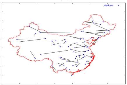
15 20 25 30 35 40 45 50 55 60 70 80 90 100 110 120 130 140 full inputs (24) stations
Figure 1: Model inferences vs true station locations: full data
In order to illustrate the behavior of the different approaches, we represent for each approach model inferences versus true station locations on different maps (figures 1,2,3,4). Triangles represent the location of the 60 stations which belong to the test set. Segments represent the location inferred by the model. In each figure, we can see that segments tend to be horizontal, which corroborates the fact that longitude inference is more difficult than latitude one.
5.4
Low Quality Data
We have seen in the previous section, that the full data approach and sym-bolic approaches achieve quite similar performances on the Chinese data example. The only advantage at this point of symbolic approaches is that the model complexity (number of weights) is lower in this case. The goal of this section is to show that models based on symbolic objects are much more robust to low quality data (data with missing values or with noisy measure-ments) than those based on the full data approach. More precisely, for each approach (standard and symbolic), we consider the MLP model estimated in the previous section: this estimation was carried out with high quality data (no missing values). Our goal is to study performances of this model when unseen data with missing values (low quality data) are submitted.
in-15 20 25 30 35 40 45 50 55 60 70 80 90 100 110 120 130 140 Mean stations
Figure 2: Model inferences vs true station locations: mean approach
15 20 25 30 35 40 45 50 55 60 70 80 90 100 110 120 130 140
Min and max
stations
15 20 25 30 35 40 45 50 55 60 70 80 90 100 110 120 130 140
Mean and standard deviation
stations
Figure 4: Model inferences vs true station locations: mean & standard devi-ation
tentionally degrade the Chinese data which belong to the test set (the training set and the validation set are not considered in this section, as we use the models which have been estimated in the previous section). Data degradation is done 3 times: the first degradation leads to data with mid-quality (half values are missing). The second degradation leads to low quality data (two thirds are missing), and finally the last degradation leads to very low quality data (three quarters are missing). Data degradation is done according to the following protocol: we consider for each meteorological station the temper-ature vector (12 coordinates) and the precipitation vector (12 coordinates). For the first degradation, we remove regularly one coordinate out of 2 for each vector (coordinates 2, 4, 6, 8, 10, 12 are missing values). Therefore the temperature vector is now a 6-dimensional vector, just as the precipitation vector. For the second degradation, we remove regularly 2 coordinates out of 3 from the original data, and the dimension of each vector is 4 (coordinates 2, 3, 5, 6, 8, 9, 11, 12 are missing values). Finally, in the third experiment we remove regularly 3 coordinates out of 4, and the dimension of each vector is 3 (coordinates 2, 3, 4, 6, 7, 8, 10, 11, 12 are missing values).
Models based on mean, min-max or mean-standard calculation can be applied directly to these new data. All we have to do is to recompute each of these quantities with the remaining values. For the full data approach, direct treatment is not so simple, as MLP models have an input dimension of 24,
which is incompatible with the data dimension (12 for the first degradation, 8 for the second degradation and 6 for the third degradation). Therefore, in order to submit these data to the full data model, we must replace each missing value by an estimate. Many well-known missing value techniques can be applied in order to compute these estimates. In order not to penalize the full data approach, we choose to replace missing values by new values computed thanks to linear interpolation. For sake of clarity, we denoteci the
ith coordinate. For the first degradation, coordinatesc
2,c4,c6,c8,c10,c12 are missing. Coordinate c2 is replaced by (c1+c3)/2. We proceed the same way for coordinatesc4, c6,c8,c10. For coordinatec12, we make use of the periodic aspect of the climate: coordinate c12 is replaced by (c1+c11)/2 (December is computed thanks to November and January of the same year). For the second degradation, we have c2 = (2c1+c4)/3 and c3 = (c1+ 2c4)/3, and so on for coordinates c5, c6, c8, c9, c11, c12. Finally for the third degradation, we have c2 = (3c1+c5)/4,c3 = (c1+c5)/2 and c4 = (c1+ 3c5)/4, and so on for coordinates c6, c7, c8, c10,c11, c12.
latitude
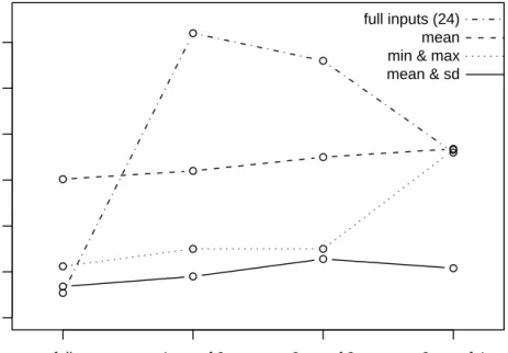
full 1 out of 2 2 out of 3 3 out of 4
1.0 1.5 2.0 2.5 3.0 3.5 4.0 full inputs (24) mean min & max mean & sd
For each of the models estimated in the first experiments, we compute the mean absolute error on the modified test set. Figure 5 summarizes per-formances obtained by the different approaches for the inference of station latitude in respect to the data degradation level. Figure 6 do the same for the longitude.
longitude
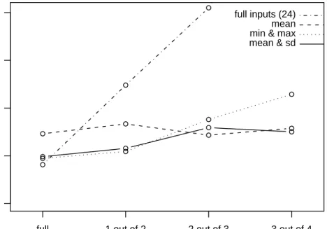
full 1 out of 2 2 out of 3 3 out of 4
0 5 10 15 20 full inputs (24) mean min & max mean & sd
Figure 6: data quality reduction: longitude
Results obtained by the different approaches leads to the following re-marks:
• first we can see that the full data approach is very sensitive to data quality compared to the other approaches. Indeed, data degradation impairs strongly performances (error evolves from 4.07 degrees to 12.4 degrees for the longitude when half values are missing, and meanwhile error evolves from 1.27 degrees to 4.1 degrees for the latitude). Other approaches are not impacted in these proportions for the same degra-dation. We can see there the outcome of using complex models, that is, models with a large number of weights: if the submitted data are close to the training data, the model achieve good performances. However, if
submitted data differs too much from the training data, performances fall down.
• we can see that performances achieved by the mean approach are quite uniform in respect to data degradation. Nevertheless, symbolic ap-proaches outperform the mean approach in almost all cases. Once again, descriptions obtained thanks to a simple averaging are too poor, which avoid MLP models from making accurate inferences.
• finally, we can see that the symbolic approach based on the (mean, sd) estimation is more robust than the one based on the (min, max) es-timation. We can explain this result by the fact that the (min, max) estimation is more sensitive to out-layers (month with unusual tempera-ture for instance) than the (mean, sd) estimation. This dependency has noticeable consequences on model inferences. We can conclude there-fore that the (mean, sd) estimation should be preferred in all cases.
6
Conclusion
We have proposed in this chapter a simple recoding solution that allows to use arbitrary symbolic inputs and outputs for multilayer perceptrons. We have shown that traditional techniques, such as weight decay regularization, can be easily transposed to the symbolic framework. Moreover the proposed approach doesn’t necessitate specific implementation: standard neural net toolbox can be used to process symbolic data. Experiments on semi-synthetic data have shown that neural processing of intervals gives satisfactory results. In future works, we plan to extend these experiments to categorical multi-valued variables and modal variables in order to validate all the recoding solutions. Finally, we plan also to study more precisely the adaptation of standard imputation methods (mean approach and k nearest neighbor ap-proach) to the symbolic framework, especially by comparing imputation on recoded variables versus imputation on symbolic variables using symbolic mean operators.
References
M. Beheshti, A. Berrached, A. de Korvin, C. Hu, and O. Sirisaengtaksin. On interval weighted three-layer neural networks. InProceedings of the 31
Annual Simulation Symposium, pages 188–194. IEEE Computer Society
C. Bishop. Neural Networks for Pattern Recognition. Oxford University Press, 1995.
H.-H. Bock and E. Diday, editors. Analysis of Symbolic Data. Exploratory
methods for extracting statistical information from complex data. Springer
Verlag, 2000.
R. Moore. Interval Analysis. Prentice-Hall, Englewood Cliffs, New Jersey, 1966.
W. H. Press, S. A. Teukolsky, W. T. Vetterling, and B. P. Flannery.
Numer-ical Recipes in C. Cambridge University Press, second edition, 1992.
F. Rossi and B. Conan-Guez. Multilayer perceptron on interval data. In A. S. K. Jajuga and H.-H. Bock, editors, Classification, Clustering, and
Data Analysis (IFCS 2002), pages 427–434, Cracow (Poland), July 2002.
Springer.
F. Rossi and B. Conan-Guez. Functional multi-layer perceptron: a nonlinear tool for functional data analysis. Neural Networks, 18(1):45–60, January 2005.
F. Rossi, N. Delannay, B. Conan-Guez, and M. Verleysen. Representation of functional data in neural networks. Neurocomputing, 64:183–210, March 2005.
T. Shiyan, F. Congbin, Z. Zhaomei, and Z. Qingyun. Two long-term instrumental climatic data bases of the people’s republic of China. Technical Report 4699, Institute of Atmospheric Physics Chi-nese Academy of Sciences, Beijing, China, September 1997. Available atftp://cdiac.ornl.gov/pub/ndp039/.
S. J. Simoff. Handling uncertainty in neural networks: An interval approach.
InInt. Conf. on Neural Networks, pages 606–610, Washington, June 1996.
IEEE.
J. ˇS´ıma. Neural Expert Systems. Neural Networks, 8(2):261–271, 1995. H. White. Connectionist nonparametric regression: mutilayer feedforward