Prediction of Internal Temperatures During Hot Summer Conditions with Time Series
Forecasting Models
Matej Gustin
1,2,*, Rob S. McLeod
1,2, Kevin J. Lomas
1,2 1School of Architecture, Building and Civil Engineering,
Loughborough University, LE11 3TU, UK
2
London-Loughborough EPSRC Centre for Doctoral Training in Energy Demand,
Loughborough University, LE11 3TU, UK
*
Correspondence: [email protected]
Abstract
A novel application using adaptive autoregressive time series forecasting with exogenous inputs (i.e. ARX) has been developed in order to provide reliable short-term forecasts of the internal temperatures in dwellings during hot summer conditions (i.e. heatwaves). The study shows that with proper selection of the predictors, based on the Akaike Information Criterion (AIC), the forecasts provide acceptable accuracy for periods up to 72 hours. The hourly results for the analysed dwellings showed a Mean Absolute Error (MAE) below 0.63°C and 0.49°C for the two case study dwellings across the 3-day forecasting period, during the 2015 heatwave. These findings point to the potential for using time series forecasting as part of an overheating warning system in buildings, especially those housing vulnerable occupants.
Introduction
Overheating in UK homes is increasingly acknowledged as a problem for UK house builders, homeowners, landlords, tenants and policy makers (NHBC, 2012; ZCH, 2016; Lomas and Porritt, 2017). Climate change projections indicate that the UK is expected to experience more frequent and more intense heat wave periods over the coming decades (Meehl and Tebaldi, 2004). Warmer than average summers coupled with an increased frequency of extreme heat wave events (Jenkins et al., 2009) pose obvious risk factors in relation to overheating in the built environment.
By 2040 average summer temperatures are expected to reach those experienced during the heatwave of 2003 (Jones et al., 2008; Public Health England, 2015), which caused over 2,000 heat-related deaths in the UK and more than 30,000 across Europe (De Bono et al., 2004). Such ‘extreme’ events are predicted to become increasingly common (Jenkins et al., 2009). Those most affected by excess heat are the elderly over the age of 75 years (ZCH, 2016). Because of the rising average life expectancy in the UK (Age UK, 2017), premature mortality rates are anticipated to increase when similar events occur in the future.
It is well known that in a temperate climate mortality increases linearly with air temperature (Hajat et al., 2006; Armstrong et al., 2010). Excess deaths can be attributed to cardiovascular causes, stroke, coronary heart diseases and respiratory causes (Huang et al., 2010). However, a study by Rooney et al. (1998) observed that mortality
during heatwaves occurring late in the summer is lower than at the beginning of the summer. This suggests that there is some seasonal acclimatisation process which increases resilience to heat stress.
Recent studies related to overheating in dwellings can be broadly divided into three categories: firstly, studies that have involved measuring internal air temperatures (and other physical variables) in order to identify and quantify the risk of overheating (Beizaee et al., 2013; Lomas and Kane, 2013; Mavrogianni et al., 2016; McLeod and Swainson, 2017); secondly, those that involved dynamic thermal simulation modelling to assess the current and future risk of overheating (Porritt et al., 2012; McLeod et al., 2013; Mavrogianni et al., 2016; Symonds et al., 2016); and lastly, studies that have used empirical data to construct forecasting models for the prediction of the indoor thermal conditions (Ríos-Moreno et al., 2007; Mustafaraj et al., 2010; Ashtiani et al., 2014; Ferracuti et al., 2017).
Dynamic simulation models, also known as white-box or physical models, are particularly indicated for use during the design phase of a building when the building characteristics and thermal proprieties of the envelope can be adequately estimated (Amara et al., 2015). Conversely, statistical models are better indicated for the predictive modelling in existing dwellings. The availability of observed data from large monitoring studies (Beizaee et al., 2013; Lomas and Kane, 2013; Firth et al., 2016; Mavrogianni et al., 2016; Symonds et al., 2016) provides the potential to develop empirical models which make predictions base on the data alone (i.e. black-box models). Black-box models are also known as statistical models (Amara et al., 2015) or machine learning tools (Foucquier et al., 2013). They can forecast the short-term future internal temperatures based solely on the external climate data and previously recorded internal temperatures. As such, black-box models are computational and resource efficient and do not require any physical information regarding the room or building fabric. Different types of black-box models can be adopted for the prediction of the internal air temperature, with the most common being Time Series and Artificial Neural Networks (Kramer et al., 2012). Statistical models rely on minimal inputs and do not require detailed parameterisation based on physical data; instead, they learn from past time-series data in order to perform forecasts, which can be updated every hour using a sliding window of data from the training and validation periods. If proven reliable, such models could
Proceedings of BSO 2018: 4th Building Simulation and Optimization Conference, Cambridge, UK: 11-12 September 2018
be usefully deployed to inform building occupants of the impending risks of overheating in a specific space. Provision of tailored information to occupants (or they carers) and/or building and facilities managers advising on the level of preventative action needed to mitigate heat-related risks is then possible.
Data selection
It is known that forecasting internal temperatures with autoregressive time series is difficult to perform where the values of future predictions fall outside the range of the past (training) values (Hyndman and Athanasopoulos, 2018). Therefore, it is essential that the development of the model is performed, tested and validated during a hot period that sufficiently stresses the model’s predictive capabilities. For that purpose, two dwellings from the REFIT Smart Home dataset (Firth et al., 2016) were selected. The houses, both located close to the town of Loughborough in the English Midlands, experienced high temperatures, but evolved different temperature profiles, during the one-day heatwave of 1st July 2015. During this
short-duration extreme hot spell, the external air temperatures exceeded 30°C in most regions of the UK (Met Office, 2015). The maximum dry-bulb temperatures during that period set a new July record, with the highest temperature of 36.7°C being observed at the Heathrow weather station (BBC, 2015; Met Office, 2015). On the hot day: dwelling A (REFIT dwelling No. 12) exhibited a sudden indoor temperature spike exceeding 30°C; dwelling B (REFIT dwelling No. 20) displayed a gradual increase in the internal temperatures with a lower peak of 27.6°, but with prolonged retention of elevated temperatures above 26°C during the following night. Both dwellings are located in the close proximity of Loughborough and hence the same external weather file was used for generating models of both dwellings. The weather data was recorded at the Loughborough University weather station at 15-minute intervals. The internal temperatures were logged at 30-minute intervals in the bedrooms. The sub-hourly data was then averaged, by centring the hourly mean values on each hour. The data adopted for the training and forecasting undertaken in this study extends across a five-week period from the 1st June
2015 to the 5th July 2015.
Simulation
Autoregressive models require that the input data used for the development of the model is stationary in order that the distribution of the observed and forecasted values is independent of time (Hyndman and Athanasopoulos, 2018). Hence, a time series can be considered stationary if the mean and variance of the data are constant (Makridakis et al., 1998) and if there are no significant trends or seasonalities in the data (Hyndman and Athanasopoulos, 2018). To objectively determine if the data is stationary, unit root tests are adopted, with one of the most popular being the Augmented Dickey-Fuller (ADF) test (Hyndman and Athanasopoulos, 2018). The
ADF unit root test was used to assess the stationarity of the input time series (with a p-value threshold of 0.01). If
the p-value of the ADF test is smaller than 0.01 (i.e. ADF
value lower than the critical value for a specific sample size) the null hypothesis of a non-stationary time series can be discarded, and the alternative hypothesis of a stationary time series accepted. Analysis of all the input time series used in this work satisfied the ADF unit root test so it can be concluded that the adopted data in this study is sufficiently stationary. As such, the input time series data does not require differentiation (d = 0) or further transformation to render it stationary. Because the use of past residuals (as input parameters in the forecasts) did not show a significant forecasting improvement, the model could be further simplified by eliminating the use of moving average terms (q = 0). Hence an autoregressive time series model with AutoRegressive inputs (p) and eXogenous (x) inputs was adopted, which can be denoted as an ARIMAX (p, d = 0, q = 0, x) model or more simply as an ARX (p, x) model.
To perform the forecasts at a specific time-step (t) and forecasting horizon (h), the model calibrates itself according to weightings applied to past internal temperatures (Tint) observed inside a specific room (or
zone), combined with the exogenous inputs of past and/or forecasted weather data, which consists of the external air temperature (Text) and global horizontal irradiance (GHI)
from the weather station. The general equation of the model can be written in the form shown in equation (1).
Tint (t+h) = c + ϕ1 Tint (t+h-1) +…+ ϕn Tint (t+h-n) + α0 Text (t+h) +…+ αn Text (t+h-n) + β0 GHI(t+h) +…+ βn GHI(t+h-n) + e (t+h) (1) where:
t hourly time step [h]
h forecasting horizon (h-step forecast) [h]
c intercept (regression constant) [°C]
n lag (delayed time step) [h]
Tint (t+h) forecasted hourly internal temperature at the time step t for the forecasting horizon h [°C]
Tint (t+h-n) observed or estimated internal temperature at lag n before the forecasting horizon h [°C]
Text (t+h-n)
observed or forecasted hourly external air temperature at lag n before the forecasting horizon h [°C]
GHI (t+h-n)
observed or forecasted Global Horizontal Irradianceat lag n before the forecasting horizon h [W/m2]
ϕn AutoRegressive coefficient (weight) of the past internal temperature (Tint) at lag n
αn eXogenous coefficient (weight) of the past/forecasted Text at lag n
βn eXogenous coefficient (weight) of the past/forecasted GHI at lag n
e (t+h) forecasting error: hourly difference between the forecasted and observed internal temp. at the time step t for the forecasting horizon h [°C]
Whilst for the one-step-ahead forecasts the model requires only observed past internal temperatures (Tint), for
multi-step-ahead forecasts the model adopts partially (when 1 <
h ≤ n) or exclusively (when h > n) the temperature estimates (i.e. forecasted internal temperatures generated at previous time steps). Similarly, the one-step-ahead forecasts require the observed past weather data (Textand
GHI) and the forecasted weather data for that specific time step (t+1). For multi-step-ahead forecasts (t+h), the model adopts partially (when 1 < h ≤ n) or exclusively (when h > n) the forecasted weather data, which is assumed to be known with sufficient accuracy.
Since an extended training period of three weeks showed more consistent and accurate forecasts than either a 1 or 2-week training period, 21 days of data were used to train the regression coefficients (ϕn, αn, βn) of the time series
models. Hence, the training period extended from the 1st
June at 00:00 to 21st June at 23:00, whilst the forecasting
period started immediately after, on the 22nd June at 00:00
(forecasting origin). For the purpose of this study the forecasts and their accuracy are analysed only during the week of the heatwave event, from 28th June at 00:00 to 4th
July at 23:00.
Approaches involving selecting all (or significant number) of the potential predictors will almost certainly not represent the best model because of the potential to include non-significant predictors; conversely, a smaller number of model predictors might lead to poor performance in multi-step-ahead forecasts. Identifying a near-optimal model manually is therefore a difficult and time-consuming (and potentially impossible) task; and consequently, it is preferable to adopt an automated parameter selection processes.
In forecasting, the Akaike Information Criterion (AIC) is often adopted for the selection of the best model from a collection of possible models. The AIC estimates the likelihood of the model to predict future values, which is penalised by the number of estimated parameters in the model (i.e. penalised likelihood). By automating the model calibration process the model can be tested with all possible combinations of input variables. The best model is then identified by selecting the combination of features (predictors) that result in the minimum value of the AIC
test. According to Hyndman and Athanasopoulos (2018), the model with the minimum value of the AIC is considered to be the optimal model for forecasting. In order to perform the model selection process in a reasonable amount of time (e.g. in less than one hour), using code written in R and using a single core processor (i.e. running the code in sequence), the lag n (i.e. the number of previous time steps of data that are considered as predictors) was limited to 5. The lagged inputs of Tint,
Text and GHI that produce the lowest AIC with the ARX
model were automatically selected. The selection process of the predictors was performed only once for each bedroom during the training period (i.e. the first 21 days) and the selected model was then adopted to perform the forecasts for that specific bedroom and dwelling. The number of AutoRegressive (p) and eXogenous (x) inputs chosen by the selection criteria for each model were
automatically assigned to the names of the output files for cross-referencing of the results tables and plots.
In ‘real-world’ applications the model would require forecasted weather data from (a) nearby meteorological station(s). Since the uncertainty of weather forecasts increases in proportion to the length of the forecasting horizon, their reliability several days ahead (particularly in a maritime climate) is questionable; as a result, using forecasting models to predict significantly long periods after the forecasting origin is likely to be unreliable. According to the Met Office, the UK short-range (1-3 days ahead) weather forecasts are considered to be extremely accurate using data that is updated several times per day (Met Office, 2016). On the other hand, medium-range (3-10 days ahead) weather forecasts provide only a general picture of the weather on a day-to-day basis. For this reason, the developed models are constrained to forecasting Tintfor the next 72 hourly time
steps (3-day forecast) after the forecasting origin. To create a multi-step forecast the model performs a one-step-ahead forecast and then iteratively completes the multi-step-ahead forecasts for the next 72 hours by adopting a recursive strategy. The model adopts a rolling forecasting origin (i.e. utilising sliding training and validation periods). This means that after each 72-hour forecast, the model training window (21 days) moves forward by one time-step (1 hour), recalibrating the regression coefficients (weights) of the previously selected predictors before recalculating the forecasts. The model automatically stops when the forecasting window (of 72 hours) reaches the end of the dataset. Once the rolling origin forecasts have been completed for the whole validation period, it is then possible to assess the forecasting accuracy.
The accuracy of a forecasting model can only be evaluated based on how well it is performing in relation to ‘new’ data (Hyndman and Athanasopoulos, 2018), i.e. not how well the model fitted the ‘past’ data during the training period. In this study, the forecasting accuracy was evaluated only during the week of the heatwave (28th June
at 00:00 to 4th July at 23:00) using scale-dependent error
metrics: Mean Bias Error (MBE), Mean Absolute Error (MAE) and Root Mean Square Error (RMSE). The adjusted coefficient of determination (R2
adj) was also
calculated for reference. Whilst calculating R2
adj during
the training period (i.e. in sample) can be useful in interpreting the goodness of fit between the model prediction and the measured data, it does not necessarilyindicate a good model for forecasting (Hyndman and Athanasopoulos, 2018). In fact, a good fit in the training period might signify an over-fitted model (i.e. the model matches the training data so closely, that it loses the ability to generalise and forecast over the entire testing/validation period) with a consequent poor forecasting performance. For these reasons, R2
adj was used
only to express the fit of the model over the testing/validation (i.e. out-of-sample) period (Hyndman and Athanasopoulos, 2018).
Knowing that the model is able to forecast accurately during a typical hot spell is not the only requisite characteristic of a reliable overheating forecasting model. Whilst sudden spikes of the internal and external temperatures can significantly decrease the short-term predictive accuracy, it is important to consider that the main purpose of the model is to inform the occupants of the time and magnitude of impending overheating risks. In reality, it is likely that when faced with prolonged and/or severe overheating the occupants might take some mitigation actions (e.g. window opening, use of air conditioning etc.) and these interventions could significantly disrupt the forecasts. Even where the model is slowly adapting to an overheating trend, sudden or unpredictable mitigation actions might significantly affect the forecasting accuracy.
In real-world applications of a model that predicts internal temperatures, occupants of the building need to understand the reliability of each forecast. Prediction intervals are commonly used to express how much uncertainty is associated with each forecast. Although forecasts are often presented as a deterministic point values, they can be better understood as the average value of a forecast distribution (Hyndman and Athanasopoulos, 2018). The predictive interval defines the range of values within which we expect the forecast to lie with a specified probability. For a normal distribution, there is a 95% probability that the actual future temperature will lie within 1.96 standard deviations of the mean and, based on the central limit theorem, this range can therefore be used as the 95% prediction interval.
In order to produce the prediction interval, the standard deviation of the h-step forecast distribution (σh) has to be
estimated first for each forecasting horizon (h). In this study, due to the large number of observations and forecasts, the σh can be assumed equal to the standard
deviation of the residuals (i.e. forecasting errors) at that specific forecasting horizon (h) assessed over the preceding week of forecasts (and progressively shorter periods are subsequently adopted until the point where the first complete week of forecasted data is yet to be realised). Once σh has been estimated it is possible to
calculate the 95% predictive intervals for each forecasting horizon h (i.e. 1h, 3h, 6h, 12h, 24h, 48h and 72h). The predictive intervals (PIh) are iteratively recalculated at
every time step (t) as shown in equation (2).
PIh = Tint (t+h) ± k σh (2)
where:
t hourly time step [h]
h forecasting horizon (h-step forecast) [h]
PIh Prediction Interval for the forecasting horizon h [°C]
k coverage factor (k = 1.96 σ for the 95% PI)
σh estimate of the standard deviation of the h-step forecast distribution [°C]
1 Since is not possible to compare the coefficients for different variables directly because they are measured on different
scales (i.e. unstandardised coefficients), they are expressed as an average percentage weight for each specific input variable Tint , Text and GHI.
The forecasts shown in this study have been performed on dwelling A and dwelling B over the same time period using the same weather data to facilitate temporal comparisons of the results.
Result analysis and discussion
The automatic selection procedure identified the ARX
models with the following orders and predictors, as being optimal:
Dwelling A:
• Identified model: ARX (5, 6)
• AutoRegressive inputs: Tint (t+h-1), Tint (t+h-2),
Tint (t+h-3), Tint (t+h-4), Tint (t+h-5)
• eXogenous inputs: Text (t+h), Text (t+h-4), GHI
(t+h), GHI(t+h-1),GHI(t+h-2), GHI(t+h-4)
Dwelling B:
• Identified model: ARX (4, 5)
• AutoRegressive inputs: Tint (t+h-1), Tint (t+h-2),
Tint (t+h-3), Tint (t+h-4)
• eXogenous inputs: Text (t+h), Text (t+h-1), Text
(t+h-2), Text (t+h-4), GHI(t+h)
It can be observed (from the above descriptions) that: the model for dwelling A has adopted more exogenous predictors based on the previous time steps of the GHI,
than Text ; the model for the dwelling B has used more
terms based on the previous time steps of the Text than
GHI. It should be noted that there are also significant differences in the coefficient weightings of the various predictors. Overall, the autoregressive terms Tint have the
most dominant relative 1 weights, whilst T
ext and GHI
have only small and very small relative weights respectively. This means also that due to the lower relative weights of the eXogenous (weather) inputs, the models are globally less sensitive to the uncertainties associated with the external weather data.
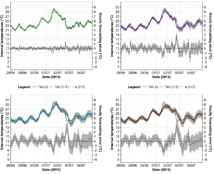
For dwelling A, the 1-hour forecasts are very accurate and almost completely aligned with the observed values, with an R2
adj of 0.989. For the 3-hour and 6-hour forecasts,
while the model is predicting accurately in relation to the peak temperature on the hottest day (1st July) (Figure 1),
there is a 2-hour lag between the forecasted and observed peaks. For longer forecasting horizons (12-72 hours), other than the delay of 1-2 hours in predicting the timing of the peak temperature, the model under-predicts the peak internal temperature on 1st July, 28.4°C (12-hour
forecast) and 28.7°C (72-hour forecast), compared to the measured peak of 30.2°C. The model is also struggling to forecast the rapid drop in the internal temperatures on the afternoon of the 2nd July (from 26.2°C at 16:00 to 21.7°C
at 21:00) at forecasting horizons of 3 or more hours. The sudden drop in temperature was caused by a rapid drop in the external temperature but perhaps occupants also opened windows to cool the room down. Overall, across
Figure 1: Dwelling A: observed - Tint(t) and predicted - Tint(t+h) hourly internal temperatures with hourly errors -
e(t+h) and the 95% predictive intervals (grey band) for 1h, 3h, 6h and 12h forecasting horizons (h).
the seven-day forecasting period, the model predicted with reasonable accuracy, with a maximum MAE of 0.63°C for the 72-hour forecasts (Table 1).
Table 1: Dwelling A: Forecasting accuracy over the analysed week of the 2015 heatwave
h R 2 adj (0-1) MBE (°C) MAE (°C) RMSE (°C) 1 0.989 0.01 0.17 0.26 3 0.910 0.03 0.44 0.62 6 0.853 0.05 0.55 0.79 12 0.831 0.08 0.60 0.85 24 0.819 0.15 0.61 0.86 48 0.853 0.26 0.59 0.78 72 0.842 0.31 0.63 0.81
For dwelling B, as for the dwelling A, the 1-hour forecasts are extremely accurate, with an R2
adjof 0.999. The 3-hour,
6-hour and 12-hour forecasts are also reasonably accurate (Figure 2). On the other hand, for longer forecasting horizons (24-72 hours), the model tends to under-predict the peak temperature and struggles to accurately predict
the retention of elevated temperatures between the 1st and
2nd July. Nonetheless, perhaps because dwelling B has a
much smoother internal temperature profile (Figure 2 cf. Figure 1), the forecasts are more accurate than those for dwelling A for all the forecasting horizons and measured by the MAE and RMSE (Table 2).
Table 2: Dwelling B: Forecasting accuracy over the analysed week of the 2015 heatwave
h R 2 adj (0-1) MBE (°C) MAE (°C) RMSE (°C) 1 0.999 -0.01 0.04 0.05 3 0.989 -0.03 0.12 0.14 6 0.955 -0.06 0.21 0.24 12 0.910 -0.12 0.28 0.33 24 0.876 -0.20 0.27 0.39 48 0.831 -0.33 0.36 0.46 72 0.729 -0.46 0.49 0.57
The tendency towards under prediction is evident in the
MBE. As for dwelling A, the MBE (in absolute terms),
Figure 2: Dwelling B: observed - Tint(t) and predicted - Tint(t+h) hourly internal temperatures with hourly errors -
e(t+h) and the 95% predictive intervals (grey band) for 1h, 3h, 6h and 12h forecasting horizons (h).
forecasting horizon h increases.
Whilst the range of the estimated 95% prediction intervals shown in the forecasts (grey band in Figures 1 and 2) temporarily increases after the heatwave, the prediction intervals consistently provide good coverage of the observed internal temperature, especially for shorter forecasting horizons (1 to 12 hours). For shorter forecasting horizons the 95% confidence region is narrow, thus demonstrating higher forecasting reliability for shorter time horizons. As noted by Hyndman and Athanasopoulos (Hyndman and Athanasopoulos, 2018), a common characteristic of prediction intervals is that they tend to gradually increase as the forecasting horizon (h) lengthens. Since the 95% predictive intervals are slowly adapting, and because they are based on past errors, they could be used to reliably inform the occupants of how reliable the forecasts are expected to be for specific forecasting horizons.
The aim of this work is to lay the foundation for an in-home device that could provide an early warning of likely elevated temperatures. Model automation is an extremely important feature of such a device since it obviates the
need for manual intervention, trial and error procedures, or model identification by an expert. Using an automatic statistical selection procedure based on the AIC criteria, it appears possible to consistently identify models with reasonable predictive ability. In principle, therefore, it might be possible to develop a device that needs only a sensor to record the internal zonal air temperature and an internet (or cellular mobile) connection to continuously access and download the weather forecast for a specific location (but see also below). After an initial training period, the device would be able to automatically select an appropriate model for the specific room before continuing to perform ongoing forecasts of the internal temperatures.
Interestingly, the parameter weightings of the derived models suggest that they are relatively immune to the uncertainty in the input weather data. Therefore, even if the derived models were to rely upon forecasted weather data from more distant meteorological stations or on interpolated data, the predictive accuracy may not degrade, which is a useful attribute if the device were deployed in remote locations.
The difficulty of making predictions during abnormal temperature events, and for longer forecasting horizons, is not surprising. Firstly, the models can only be trained based on past events the prediction of sudden, rare and extreme events will always be difficult. Secondly, during such events, the occupants of homes may behave differently; abnormally even. Mitigating actions during a heatwave could include, opening windows and even doors, closing the curtains during the day, turning on portable fans or even using portable air conditioning units. Models learn slowly and although such actions will be incorporated in the model forward predictions, even for only three hours ahead will be degraded. Additional sensors, for example, to detect window opening, could enhance the model, but this adds cost, complexity and only deals with one of the possible occupant behaviours. Rather than adding complexity to the monitoring system, future work will focus on further improvements to the modelling procedure and understanding the factors that affect the models’ predictive accuracy. One approach to modelling that will be explored is the use of Non-linear neural network ARX models (i.e. NARX models). Whereas this work has examined two, specifically-selected rooms, in one town, with hourly temperatures recorded over just one summer period, future endeavours will entail testing the modelling process and quantifying the models’ accuracy for many more rooms, households, dwelling types and locations.
Ultimately, it is hoped that forecasts of sufficient reliability could be provided to vulnerable occupants (and their carers) several days in advance (24-72 hours), which would allow occupants and emergency services adequate time to prepare a response. The very reliable shorter-term forecasts (1-12 hours) would facilitate the coordinated and targeted deployment of these services.
Conclusions
The potential for numerical models to predict internal temperatures during heatwaves has been investigated using hourly data form two bedrooms, in two houses located close to the town of Loughborough in the UK Midlands. During the monitoring period, there was a one-day heat wave during which the external dry-bulb temperature exceeded 35°C. The AIC was adopted to automatically identify a near optimal forecasting model, immediately prior to the period of hot weather, that is tailored to the specific room and dwelling. Recursive multi-step-ahead forecasts for the next 72 hours were performed with a rolling origin in order to provide predictions at different forecasting horizons for the week of the heatwave allowing validation of the model over that period. The MBE and R2
adj were calculated to evaluate the
bias and out-of-sample fit of the model respectively. The
MAE and RMSE were used to assess the forecasting accuracy of the model over the validation period, and 95% prediction intervals were computed to express the reliability of the forecasts at different forecasting horizons. The adopted statistical selection procedure showed that is possible to automatically identify a near optimal forecasting model, prior to a period of hot
weather, that is tailored to a specific room and dwelling. The results of this study suggest that statistical black-box models (e.g. ARX forecasting time series) can be used for the forecasting of the internal temperature profile in dwellings several days in advance with an acceptable forecasting accuracy. Moreover, for shorter forecasting horizons (1-12 hours) the models are capable of producing significantly more accurate and reliable predictions even during extreme summer conditions.
Nomenclature
AIC Akaike’s Information Criterion ADF test Augmented Dickey-Fuller test
ARIMAX (p, d, q, x)
AutoRegressive Integrated Moving Average with eXogenous inputs
p AutoRegressive inputs: number of past observed values considered as predictors
d Integration order: adopted order of
differencing to make the input data stationary
q Moving Average (MA) order: number of past residuals considered as predictors
x eXogenous inputs: number of external variables adopted as predictors
ARX (p, x)
AutoRegressive time series with eXogenous inputs (d = 0; q = 0)
e (t+h) forecasting error: the hourly difference between the forecasted and observed internal temperatures at the time step t for the forecasting horizon h [°C]
h forecasting horizon (h-step forecast) [h]
MAE Mean Absolute Error [°C]
MBE Mean Bias Error [°C]
n lag (delayed time steps of the inputs) [h]
NARX Non-linear neural network ARX model PIh 95% predictive interval for the forecasting
horizon h [°C]
R2adj adjusted coefficient of determination [0-1]
RMSE Root Mean Squared Error [°C]
t hourly time step [h]
Tint (t) observed hourly internal temperature at the time step t [°C]
Tint (t+h) forecasted hourly internal temperature at the time step t for the forecasting horizon h[°C]
Acknowledgements
This research was made possible by EPSRC support for the London-Loughborough CDT in Energy Demand (grant EP/H009612/1). Monitored data, indispensable to this study, was made available by the open access REFIT Smart Home dataset(Firth et al., 2016), which was funded by the EPSRC (grant EP/K002457/1).
References
Age UK (2017). Later Life in the United Kingdom. Amara, F., Agbossou, K., Cardenas, et al. (2015).
Comparison and Simulation of Building Thermal Models for Effective Energy Management. Smart
Grid and Renewable Energy 6(April), pp. 95–112. Armstrong, B.G., Chalabi, Z., Fenn, B., Hajat, S., et al.
(2010). The association of mortality with high temperatures in a temperate climate : England and Wales. Journal of Epidemiology and Community Health 65(4), p. 340.
Ashtiani, A., Mirzaei, P.A. and Haghighat, F. (2014). Indoor thermal condition in urban heat island: Comparison of the artificial neural network and regression methods prediction. Energy and Buildings 76, pp. 597–604.
BBC (2015). Hottest July day ever recorded in UK. Beizaee, A., Lomas, K.J. and Firth, S.K. (2013).
National survey of summertime temperatures and overheating risk in English homes. Building and Environment 65, pp. 1–17.
De Bono, A., Giuliani, G., Kluster, S. and Peduzzi, P. (2004). Impacts of summer 2003 heat wave in Europe. Environment Alert Bulletin UNEP (August). Ferracuti, F., Fonti, A., Ciabattoni, L., Pizzuti, S., et al.
(2017). Data-driven models for short-term thermal behaviour prediction in real buildings. Applied Energy 204, pp. 1375–1387.
Firth, S., Kane, T., Dimitriou, V., Hassan, T., et al. (2016). REFIT Smart Home dataset.
Foucquier, A., Robert, S., Suard, F., et al. (2013). State of the art in building modelling and energy
performances prediction: A review. Renewable and Sustainable Energy Reviews 23, pp. 272–288. Hajat, S., Armstrong, B., Baccini, M., et al. (2006).
Impact of High Temperatures on Mortality Is There an Added Heat Wave Effect ? 17(6), pp. 632–638. Huang, W., Kan, H. and Kovats, S. (2010). The impact of the 2003 heat wave on mortality in Shanghai , China. Science of the Total Environment, The
408(11), pp. 2418–2420.
Hyndman, J.R. and Athanasopoulos, G. (2018).
Forecasting: principles and practice. 2nd ed. OTexts.
Jenkins, G.J., Perry, M.C. and Prior, M.J. (2009). The climate of the UK and recent trends. Met Office Hadley Centre, Exeter, UK.
Jones, G.S., Stott, P.A. and Christidis, N. (2008). Human contribution to rapidly increasing frequency of very warm Northern Hemisphere summers. Journal of Geophysical Research Atmospheres 113(2), pp. 1– 17.
Kramer, R., van Schijndel, J. and Schellen, H. (2012). Simplified thermal and hygric building models: A literature review. Frontiers of Architectural Research 1(4), pp. 318–325.
Lomas, K. and Kane, T. (2013). Summertime temperatures and thermal comfort in UK homes.
Building Research and Information 41(3), pp. 259–
280.
Lomas, K.J. and Porritt, S.M. (2017). Overheating in buildings: lessons from research. Building Research & Information , pp. 1–18.
Makridakis, S., Wheelwright, C.S. and Hyndman, J.R. (1998). Forecasting: Methods and Applications. 3rd ed. John Wiley & Sons, Inc.
Mavrogianni, A., Pathan, A., Oikonomou, E., Biddulph, P., et al. (2016). Inhabitant actions and summer overheating risk in London dwellings. Building Research & Information 0(0), pp. 1–24. McLeod, R., Hopfe, C. and Kwan, A. (2013). An
investigation into future performance and
overheating risks in Passivhaus dwellings. Building and Environment 70, pp. 189–209.
McLeod, R. and Swainson, M. (2017). Chronic
overheating in low carbon urban developments in a temperate climate. Renewable and Sustainable Energy Reviews 74, pp. 201–220.
Meehl, G.A. and Tebaldi, C. (2004). More Intense , More Frequent , and Longer Lasting Heat Waves in the 21st C. Science 305(August), pp. 994–997. Met Office (2015). Heatwave 1 July 2015 - Met Office. Met Office (2016). 10 day weather forecast - Met Office. Mustafaraj, G., Chen, J. and Lowry, G. (2010).
Development of room temperature and relative humidity linear parametric models for an open office using BMS data. Energy and Buildings 42(3), pp. 348–356.
NHBC (2012). Overheating in new homes; A review of the evidence.
Porritt, S.M., Cropper, P.C., Shao, L. and Goodier, C.I. (2012). Ranking of interventions to reduce dwelling overheating during heat waves. Energy and
Buildings 55, pp. 16–27.
Public Health England (2015). Heatwave plan for England: Protecting health and reducing harm from severe heat and heatwaves. London.
Ríos-Moreno, G.J., Trejo-Perea, M., Castañeda-Miranda, R., Hernández-Guzmán, V.M., et al. (2007).
Modelling temperature in intelligent buildings by means of autoregressive models. Automation in Construction 16(5), pp. 713–722.
Rooney, C., McMichael, A.J., Kovats, R.S. and
Coleman, M.P. (1998). Excess mortality in England and Wales, and in Greater London, during the 1995 heatwave. Journal of Epidemiology & Community Health 52(8), pp. 482–486.
Symonds, P., Taylor, J., Mavrogianni, A., et al. (2016). Overheating in English dwellings: comparing modelled and monitored large-scale datasets.
Building Research and Information 45(1–2), pp. 195–208.