printf("%s %ld bytes in %.1f seconds", direction, amount, delta);
printf(" [%.0f bits/sec]", (amount*8.)/delta); }
On the implementation front, when you consider alternatives, you should always use measurement data to evaluate them; then, when you write the corresponding code, measure its performance-critical components early and often, to avoid nasty surprises later on.
You will read more about measurement techniques in the next section. In many cases, a major source of performance improvements is the use of a more efficient algorithm; this topic is covered in Section 4.2. Having ruled out important algorith-mic inefficiencies, you can begin to look for expensive operations that impact your program’s performance. Such operations can range from expensivecpuinstructions to operating system and peripheral interactions; all are covered in Sections 4.3–4.6. Finally, in Section 4.7, we examine how caching is often used to trade memory space for execution time.
Exercise 4.1 Choose five personal productivity applications and five infrastructure applica-tions your organization relies on. For each application, list its most important time-related attribute.
Exercise 4.2 Your code provides a horrendously complicated yet remarkably efficient imple-mentation of a simple algorithm. Although it works correctly, measurements have demonstrated that a simple call to the language’s runtime library implementation would work just as well for all possible input cases. Provide five arguments for scrapping the existing code.
4.1 Measurement Techniques
Humans are notoriously bad at guessing why a system is exhibiting a particular time-related behavior. Starting your search by plunging into the system’s source code, looking for the time-wasting culprit, will most likely be a waste of your time. The only reliable and objective way to diagnose and fix time inefficiencies and problems is to use appropriate measurement tools. Even tools, however, can lie when applied to the wrong problem. The best approach, therefore, is to first evaluate and understand the type of workload a program imposes on your system and then use the appropriate tools for each workload type to analyze the problem in detail.
4.1.1 Workload Characterization
A loaded program on an otherwise idle system can at any time instance be in one of the three different states:
1. Directly executing code. The time spent directly executing code is termed user time(u), denoting that the process operates in the context of its user. 2. Having the kernel execute code on its behalf. Correspondingly, the time the
kernel devotes to executing code in response to a process’s requests is termed system time(s), orkernel time.
3. Waiting for an external operation to complete. Operations that cause a pro-gram to wait are typically read or write requests to slow peripherals, such as disks and printers, input from human users, and communication with other processes, often over a network link. This time is referred to asidle time. The total time a program spends in all three states is termed the real time(r) the program takes to operate, often also referred to as the program’s wall clock time: the time we can measure using a clock on the wall or a stopwatch. The sum of the program’s user and system time is also referred to ascputime.
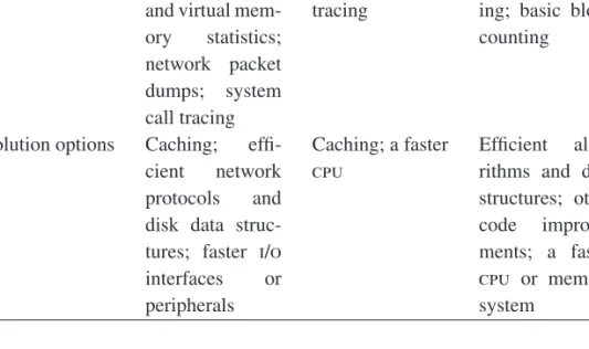
The relationship among the real, kernel, and user time in a program’s (or com-plete system’s) execution is an important indicator of its workload type, the relevant diagnostic analysis tools, and the applicable problem-resolution options. You can see these elements summarized in Table 4.1; we analyze each workload type in a separate section.
On Unix-type systems, you can specify a process as an argument of thetime11 command to obtain the user, system, and real time the process took to its completion. On Windows systems, thetaskmgrcommand can list a process’scputime and show a chart indicating the time the system spends executing kernel code. For nontermi-nating processes, you will have to obtain similar figures on Unix systems through the commonly available topcommand. On an otherwise unloaded system, you can easily determine a process’s user and system time from the corresponding times of the whole system. When analyzing a process’s behavior, carefully choose its execution environment: Execute the process either in a realistic setting that reflects the actual intended use or on an unloaded system that will not introduce spurious noise in your measurements.
Table 4.1Timing Profile Characterization, Diagnostic Tools, and Resolution Options
Timing Profile ru+s s > u ur
Characterization i/o-bound Kernel-bound cpu-bound
Diagnostic tools Disk, network, and virtual mem-ory statistics; network packet dumps; system call tracing System call tracing Function profil-ing; basic block counting
Resolution options Caching; effi-cient network protocols and disk data struc-tures; faster i/o interfaces or peripherals
Caching; a faster cpu
Efficient algo-rithms and data structures; other code improve-ments; a faster cpu or memory system
4.1.2 I/O-Bound Tasks
Programs and workloads whose real timer is a lot larger than theircputimeu+s are characterized asi/o-bound. Such programs spend most of their time idle, waiting for slower peripherals or processes to respond. Consider as an example the task of creating a copy of the word dictionary on a diskless system with annfs-mounted disk and a 10mb/s network interface:
$ /usr/bin/time cp /usr/share/dict/words wordcopy
5.68 real 0.00 user 0.32 sys
It would be futile to try to analyze thecp12command, looking for optimization op-portunities that would make it execute faster than the 5.68 seconds it took. The results of thetimecommand indicate thatcpspent negligiblecputime; for 94% of its clock time, it was waiting for a response from thenfs-mounted disk.
The diagnostic tools we use to analyzei/o-bound tasks aim to find the source of the bottleneck and any physical or operational constraints affecting it. The physical constraint could be lagging responses from a genuinely slow disk or the network;
the corresponding operational constraints could be the overloading of the disk or the network with other requests that are not part of our workload. On Unix systems, the iostat,13netstat,14nfsstat,15andvmstat16commands provide summaries and contin-uous textual updates of a system’s disk and terminal, network, and virtual memory performance. On Windows systems, the management console performance monitor (invoked as theperfmoncommand) can provide similar figures in the form of detailed charts. After we find the source of the bottleneck, we can either improve the hardware performance of the corresponding peripheral (by deploying a faster one in its place) or reduce the load we impose on it. Strategies for reducing the load include caching (discussed in Section 4.7) and the adoption of more efficient disk data structures or network protocols, which will minimize the expensive transactions. We discuss how these elements relate to specific source code instances in Section 4.5.
Analyzing the disk performance on thenfsserver hosting thewordsfile in our example usingiostatshows the load on the disk to be quite low:
ad0 KB/t tps MB/s 0.00 0 0.00 32.80 15 0.47 27.12 24 0.63 37.31 26 0.94 73.60 10 0.71 35.24 33 1.14 25.14 21 0.51 7.00 4 0.03 0.00 0 0.00
The load never exceeded 1.14mb/s, well below even the lowly 3.3mb/spio17mode 0 transfer mode limit. Therefore, the problem is unlikely to be related to the actual disk i/o. However, usingnetstatto monitor the networki/oon the diskless machine does provide us with an insight:
13netbsdsrc/usr.sbin/iostat 14netbsdsrc/usr.bin/netstat 15netbsdsrc/usr.bin/nfsstat 16netbsdsrc/usr.bin/vmstat
17The programmed input/output mode is a legacyatapihard disk data transfer protocol that supports data
transfer rates ranging from 3.3mb/s (piomode 0) to 16.6mb/s (piomode 4). Modernatapidrives typically operate using the Ultra-dmaprotocol, supporting transfer rates up to 133mb/s.
input (Total) output
packets errs bytes packets errs bytes colls
1 0 60 1 0 250 0 210 0 237744 204 0 230648 113 417 0 515196 418 0 513722 324 383 0 467208 402 0 496650 292 368 0 451418 381 0 470212 259 425 0 519588 430 0 515714 301 400 0 488434 400 0 496816 287 9 0 6106 15 0 11886 7 1 0 60 1 0 138 0
The maximum network throughput attained is 7.9mb/s,18which is very near the limit of what the particular machine’s half-duplex 10mb/s ethernet interface can deliver in practice. We can therefore safely say that the operation efficiency of the particular command invocation is bound by the capacity of the machine’s network interface. Minimizing the network traffic (by adding, for example, a local disk and keeping copies of the data on it) or improving the network interface (for example, to 100mb/s) will most probably correct the particular deficiency.
In some cases, a more detailed examination of thei/ooperations may be required to locate the problem. Two tool categories that will provide such details are system call tracers and network packet-monitoring tools. On Unix systems, you will find such commands asstrace,dtrace,truss,ltrace,19tcpdump, and ethereal;20for Windows systems, you will have to download such programs asapispy andwindump. Your objective here is to examine either the sheer volume of the corresponding transactions or the time a single transaction takes to complete. Most tools provide options for time stamping each transaction, thus providing you with an easy way to reason about the program’s behavior.
Consider, for example, the performance of the Apachelogresolve21 command. The command reads a web server log and replaces numericip addresses with the corresponding host name. Examining its operation withtimereveals that it spends 99.99%22of its time sitting idle:
$ /usr/bin/time logresolve <httpd-access.log >/dev/null
1230.55 real 0.04 user 0.03 sys
18Calculated as 8(519,588+515,714)/1,0242. 19freshmeat.net/projects/ltrace
20http://www.ethereal.com 21apache/src/support/logresolve.c
The output of thenetstatcommand also shows an (almost) idle network connection:
input (Total) output
packets errs bytes packets errs bytes colls
7 0 486 8 0 108 0 14 0 229 11 0 383 0 3 0 336 3 0 324 0 3 0 216 4 0 301 0 3 0 667 3 0 216 0 6 0 98 2 0 301 0
However, obtaining a network packet dump with tcpdump and examining the timestamps of a single name lookup operation reveal that this may require up to 150 ms:23
16:15:33.283221 istlab.dmst.aueb.gr.1024 > gns1.nominum.com.domain: 9529 [1au] PTR? 105.199.133.198.in-addr.arpa. (57)
16:15:33.433305 gns1.nominum.com.domain > istlab.dmst.aueb.gr.1024: 9529*- 1/2/0 (122) (DF) [tos 0x80]
Ignoring the effects of caching (whichlogresolvedoes perform),24we can easily see that processing a 10 million log file may require 17 days.25Thus,logresolve’s caching is certainly a worthwhile investment.
4.1.3 Kernel-Bound Tasks
Programs and workloads whose system time s is larger than their user timeucan be characterized askernel-bound. Strictly speaking, the kernel-bound tasks are also cpu-bound in the sense that improving the processor’s speed will often increase their performance. However, we treat such programs as a separate class because they require different diagnostic and resolution techniques. Your objective when dealing with a kernel-bound task is first to determine what kernel system calls the task performs. A system call tracing utility, such asstrace or apispy, will be your tool of choice here.26Such a program will provide you with a list of all the system calls a process has performed. As we discuss in Section 4.4, system calls are relatively expensive
23Calculated as(433,305−283,221)/1,000. 24apache/src/support/logresolve.c:32–34 25Calculated as 0.150×10⁷/60/60/24.
26Don’t confuse system call tracing with the program comprehension human activity with the same name
operations; therefore, you will then browse the system call list to see whether any calls could be eliminated by the use of appropriate user-level caching strategies.
Consider, as an example, running the directory listinglscommand to recursively list the contents of a large directory tree:
$ /usr/bin/time ls -lR >/dev/null
4.59 real 1.28 user 2.73 sys
We can easily see thatls spends twice as much time operating in the context of the kernel than the time it spends executing user code. Examining the output of the stracecommand, we see that for listing 7,263 files,lsperforms 18,289 system calls. Thestracecommand also provides a summary display, which we can use to see the number of different system calls and the average time each one took:
% time seconds usecs/call calls errors syscall
--- --- --- --- --- ---42.52 5.604588 994 5638 lstat 13.95 1.838295 842 2183 open 12.38 1.632320 599 2727 fstat 12.37 1.630742 747 2182 fchdir 11.41 1.503261 690 2180 close 2.94 0.387360 353 1096 getdirentries [...]
Armed with that information, we can reason that ls performs an lstat or fstat system call for every file it visits.
Based on those results, we can look at the source to find the cause of the various statcalls:27
if (!f_inode && !f_longform && !f_size && !f_type && sortkey == BY_NAME)
fts_options |= FTS_NOSTAT;
The preceding snippet tells us that by omitting the “long” option, we will probably eliminate the correspondingstat calls. The improvement in the execution perfor-mance figures corroborates this insight:
$ /usr/bin/time ls -R >/dev/null
1.08 real 0.28 user 0.77 sys