What determines mutual fund size?
Yonathan Schwarzkopf
∗†and J. Doyne Farmer
†‡December 12, 2009
Abstract
The mutual fund industry manages about a quarter of the assets in the U.S. stock market and thus plays an important role in the U.S. economy. The question of how much control is concentrated in the hands of the largest players can be quantitatively discussed in terms of the tail behavior of the mutual fund size distribution. We study the distribution empirically and show that the tail is better described by a log-normal than a power law, indicating less concentration than, for example, personal wealth. We postulate that the reasons for this stem from market efficiency and the stochastic nature of fund returns; they otherwise have very little to do with investor choice. To demon-strate this we study mutual fund entry, exit and growth empirically and develop a stochastic model. Under simplifying assumptions we obtain a time-dependent analytic solution. The distribution evolves from a log-normal into a power law only over long time scales, sug-gesting that log-normality comes about because the industry is still young. Numerical solutions under more realistic conditions support this conclusion and give good agreement with the data. Our study shows that, while mutual funds behave in many respects like other firms, there some respects in which they are quite unusual. Surpris-ingly, it appears that transaction costs and investor choice play only a minor role in determining fund size.
∗Department of Physics, California Institute of Technology,
1200 E California Blvd, mc 103-33 Pasadena, CA 91125
†Santa Fe Institute, 1399 Hyde Park Road, Santa Fe, NM 87501 ‡Luiss Guido Carli, Viale Pola 12 00198,
ROMA Italy
1
Introduction
In the past decade the mutual fund industry has grown rapidly, moving from 3% of taxable household financial assets in 1980, to 8% in 1990, to 23% in 20071. In absolute terms, in 2007 this corresponded to 4.4 trillion
USD and 24% of U.S. corporate equity holdings. Mutual funds account for a significant fraction of trading volume in financial markets and have a substantial influence on prices. Moreover, large players such as institutional investors are known to play an important role in the market [Corsetti et al., 2001] and it was recently hypothesized that the fund size distribution is of fundamental importance in explaining both the heavy tailed trading volume distribution and the heavy tailed price return distribution observed across different assets2. This raises the question of who has this influence: Are
mutual fund investments concentrated in a few dominant large funds, or spread across many funds of similar size? What are the economic mechanisms that determine this?
This question can be addressed quantitatively in terms of the upper tails of the mutual fund size distribution. The two competing hypotheses usually made in studies of firms in general are a Zipf (power law) distribution, which is so heavy tailed that none of its moments exist, vs. a log-normal distri-bution, for which all the moments exist. For mutual funds we resolve this empirically using the CRSP data set and find that the equity fund size dis-tribution is much better described by a log-normal disdis-tribution. This implies less dominance by the largest funds.
This naturally leads to the question of why this is true. One would naively think (as we did) that investor choice would be a key determinant of fund size. At the level of individual funds this is almost certainly true. Investors make their choice based on factors such as past performance, advertising, fees, and investment fads, that are potentially fertile ground for behavioral economics. This is surely important in determining the size of individual
funds. Our results, in contrast, suggest that for the distribution of fund sizes the details of individual choice are not important.
1 Data is taken from the Investment Company Institute’s 2007 fact book available at
www.ici.org.
2 The equity fund size distribution was argued to be responsible for the observed
distribution of trading volume [Levy et al., 1996; Solomon and Richmond, 2001], and Gabaix et al. have argued that it is important for explaining the distribution of price returns [Gabaix et al., 2003; Gabaix et al., 2006].
A hypothesis put forth by Berk and Green [2004] is that the sizes of mu-tual funds are determined by a combination of the distribution of skill of mutual fund managers and transaction costs. All else being equal, larger funds must make bigger transactions. Due to market impact, bigger trans-actions incur larger costs per share, and at sufficiently large size this should diminish a fund’s performance and make it less able to attract funds. Under the assumption of market efficiency, a fund with superior performance before transaction costs will grow until its after transaction cost returns are equiv-alent to those of other funds. This hypothesis is compelling and plausible, but as we discuss in more detail later, the empirical evidence suggests that it is not consistent with the data.
We offer the competing hypothesis that fund size is a diffusive process, and can be well-understood by treating changes in fund size as random. We are working in the tradition of stochastic models for firm size initiated by Gibrat, Simon and Mandelbrot, and elaborating on earlier work by Gabaix et al.3. Our treatment is new in that we find a time-dependent solution. We
argue that this is essential for understanding the empirical data. In a sense that we make precise, the diffusion of fund size is slow, and gets even slower as a fund gets bigger. As we show, since funds are entering and exiting, under stationary conditions the distribution will eventually become a power law, but this takes a very long time. This is exacerbated by the fact that the diffusion slows down as a fund gets larger. As a result the typical time to approach the asymptotic heavy tailed power law distribution is the order of a century. In the meantime the transient distribution has an essentially log-normal upper tail.
Our theory suggests that fund size is a robust property for which investor choice plays at most a minor role. A critic might say that this implies that the whole phenomenon of fund size has “no economic content”. We view this as a positive attribute of our theory: It implies that its conclusions are very robust, depending neither on rationality, nor on the idiosyncrasies of human behavior.
Our results are interesting in the broader context of the literature on firm
3A similar model yielding a steady state power law distribution, was originally proposed
by Gabaix et al. [Gabaix et al., 2003]. Their steady state treatment lacks both an empirical verification of the power law hypothesis and a justification for thet→ ∞limit taken while solving the model. A similar argument for the power law steady state in a simple entry and exit process is described in [Mitzenmacher, 2004]. Neither of these solved the more general time dependent case, as we have here.
size. Mutual funds provide a particularly good type of firm to study because there are a large number of funds and their size is accurately recorded. It is generally believed that the resulting size distribution from aggregating across industries has a power law tail that roughly follows Zipf’s law, but for individual industries the tail behavior is debated4. A large number of
stochastic process models have been proposed to explain this5. Our empirical results show that in many respects mutual funds behave like typical firms. In particular, they show the same power law decay in the diffusion rate vs. size that has been observed for other types of firms6. However, mutual funds are distinctive in that, unlike other types of firms that have been studied, in the large size limit the mean and standard deviation of the growth rate do not decay to zero, but rather approach a positive limit. This has a simple economic interpretation: In the large size limit, a fund continues to grow in size simply due to its own performance, even without further inflows of capital7. As our analytic treatment of this problem shows, this makes a crucial difference in the asymptotic behavior. It implies that after the passage of a sufficient length of time, the size distribution for mutual funds should approach a power law, whereas other firms should approach a stretched exponential, which has relatively thin tails (thinner than those of a log-normal). Thus for most firms the tails should get thinner with time, but for mutual funds they should become fatter. This does not have much effect on the current empirical distribution, however, since because of the slow diffusion mentioned earlier, over timescales less than a century both mutual funds and other firms should remain roughly log-normal.
The paper is organized as follows. Section 2 describes the data used
4 Some studies have found that the upper tail is a log-normal [Simon, Herbert A. and
Bonini, Charles P., 1958; Stanley et al., 1995; Y. and A., 1977; Stanley et al., 1996; Amaral et al., 1997a; Bottazzi and Secchi, 2003a; Dosi, 2005] while others have found a power law [Axtell, 2001; Bottazzi and Secchi, 2003a; Dosi, 2005]
5 For past stochastic models see [Gibrat, 1931; Simon, 1955; Simon, Herbert A. and
Bonini, Charles P., 1958; Mandelbrot, 1963; Y. and A., 1977; Sutton, 1997; Gabaix et al., 2003; Gabaix et al., 2003]
6 For the main body of work on the size dependence of firm growth rate fluctuations
see[Stanley et al., 1995, 1996; Amaral et al., 1997a; Bottazzi, 2001a; Bottazzi and Secchi, 2003a, 2005a; Dosi, 2005; De Fabritiis et al., 2003a]
7 Under the Berk and Green theory [2004], this should be irrational – investors should
remove their funds and reallocate them to smaller funds. Thus in this sense there is some behavioral dependence on the solution, though since the convergence is so slow, it makes no difference in the current mutual fund distribution. See the discussion in Section 6.
for the empirical study described in Section 3. The underlying dynamical processes responsible for the size distribution are discussed in Section 4 and are used to develop the model discussed in Section 5. Section 5.1 presents the solution for the number of funds and Section 5.2 presents the solution for the size distribution. In Section 5.3 we present simulation results of the proposed model and compare them to the empirical data. In section 6 we discuss the incompatibility of the Berk and Green [2004] hypothesis with the empirical data and our hypothesis. Finally Section 7 presents our conclusions.
2
Data Set
We analyze the CRSP Survivor-Bias-Free US Mutual Fund Database. Be-cause we have daily data for each mutual fund, this database enables us not only to study the distribution of mutual fund sizes in each year but also to investigate the mechanism of growth. We study the data from 1991 to 20058. We define an equity fund as one whose portfolio consists of at least 80% stocks. The results are not qualitatively sensitive to this, e.g. we get essentially the same results even if we use all funds. The data set has monthly values for the Total Assets Managed (TASM) by the fund and the Net Asset Value (NAV). We define the size sof a fund to be the value of the TASM, measured in millions of US dollars and corrected for inflation relative to July 2007. Inflation adjustments are based on the Consumer Price Index, published by the BLS.
3
The observed distribution of mutual fund
sizes
Despite the fact that the mutual fund industry offers a large quantity of well-recorded data, the size distribution of mutual funds has not been rigorously studied. This is in contrast with other types of firms where the size distribu-tion has long been an active research subject. The fact that the distribudistribu-tion is highly skewed and heavy tailed can be seen in Figure 1, where we plot
8 There is data on mutual funds starting in 1961, but prior to 1991 there are very few
entries. There is a sharp increase in 1991, suggesting incomplete data collection prior to 1991.
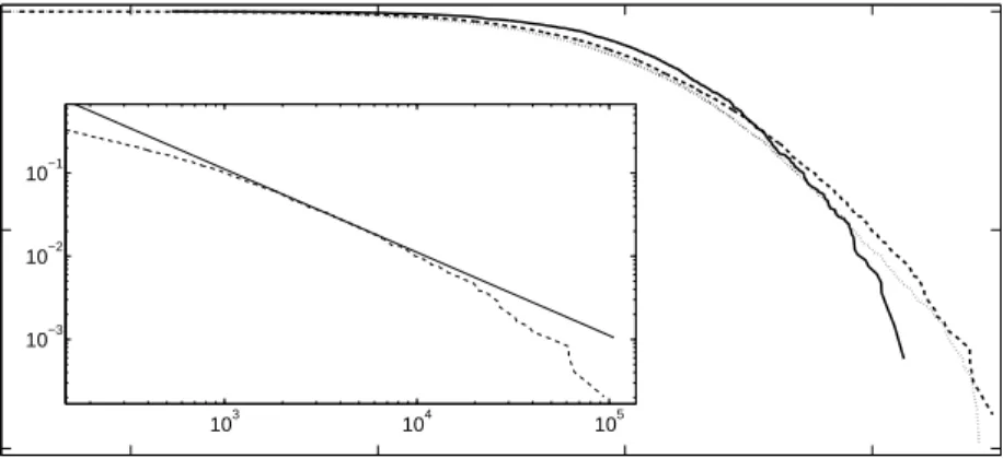
10−2 100 102 104 100 10−2 10−4 X P(s>X) 103 104 105 10−3 10−2 10−1
Figure 1: The CDF for the mutual fund size s (in millions of 2007 dollars) is plotted with a double logarithmic scale. The cumulative distribution for funds existing at the end of the years 1993, 1998 and 2005 are given by the full, dashed and dotted lines respectively.
Inset: The upper tail of the CDF for the mutual funds existing at the end of 1998 (dotted line) is compared to an algebraic relation with exponent −1 (solid line).
the cumulative distribution of sizes P(s > X) of mutual fund sizes in three different years.
The exact functional form for the distribution of fund size is still debated. The two principal competing hypotheses are that the tail of the size distri-bution p(s) is either log-normal or a power law. Log-normality means that logs has a normal distribution, while power law means that the cumulative distribution P for larges is of the form9
P(s > X)∼X−ζs,
where ζs > 0. In the special case ζs ≈ 1 a distribution P is said to obey
Zipf ’s law. Power laws have the property that moments of higher order
than α do not exist, so if a distribution follows Zipf’s law its right skewness is so extreme that the mean is on the boundary where it becomes infinite and there is no such thing as an “average fund size”. In contrast, for a log-normal all the moments exist. From the point of view of extreme value theory this distinction is critical, since it implies a completely different class of tail behavior10.
A visual inspection of the mutual fund size distribution suggests that it does not follow Zipf’s law11. To see this, in the inset of Figure 1 we
compare the tail for funds with sizes s > 102 million to a power law s−ζs,
with ζs = −1. Whereas a power law corresponds to a straight line when
plotted on double logarithmic scale, the data show substantial and consistent downward curvature. In the remainder of this section we make more rigorous tests that back up the intuitive impression given by this plot, indicating that the data are not well described by a power law.
9 We denote scaling by f(x)∼g(x) which means that the two terms are proportional
for large x, i.e. f(x)∝g(x) for largex.
10 According to extreme value theory a probability distribution can have only four
possible types of tail behavior. The first three correspond to distributions with finite support, thin tails, and tails that are sufficiently heavy that some of the moments do not exist, i.e. power laws. The fourth category corresponds to distributions that in a certain sense do not converge; it is remarkable that most known distributions fall into one of the first three categories [Embrechts et al., 1997].
11 Previous work on the size distribution of mutual funds by Gabaix et al. [Gabaix
et al., 2003; Gabaix et al., 2003; Gabaix et al., 2006] argued for a power law while we argue here for a log-normal.
3.1
Is the tail a power law?
To test the validity of the power law hypothesis we use the method developed by Clauset et al. [2007]. They use the somewhat strict definition12 that the
probability density function p(s) is a power law if there exists an smin such
that for sizes larger thansmin, the functional form of the densityp(s) can be
written p(s) = ζs smin s smin −(ζs+1) , (1)
where the distribution is normalized in the interval [smin,∞). There are two
free parameters smin and ζs. This crossover size smin is chosen such that it
minimizes the Kolmogorov-Smirnov (KS) statistic D, which is the distance between the CDF of the empirical data Pe(s) and that of the fitted model Pf(s), i.e.
D= max
s≥smin
|Pe(s)−Pf(s)|.
Using this procedure we estimateζs and smin for the years 1991- 2005 as
shown in Table 1. The values of ζs computed in each year range from 0.78
to 1.36 and average ¯ζs = 1.09±0.04. If indeed these are power laws this is
consistent with Zipf’s law. But of course, merely computing an exponent and getting a low value does not mean that the distribution is actually a power law.
To test the power law hypothesis more rigorously we follow the Monte Carlo method utilized by Clauset et al. Assuming independence, for each year we generate 10,000 synthetic data sets, each drawn from a power law with the empirically measured values of smin and ζs. For each data-set we
calculate the KS statistic to its best fit. The p-value is the fraction of the data sets for which the KS statistic to its own best fit is larger than the KS statistic for the empirical data and its best fit.
The results are summarized in Table 1. The power law hypothesis is rejected with two standard deviations or more in six of the years and rejected at one standard deviation or more in twelve of the years (there are fifteen in total). Furthermore there is a general pattern that as time progresses the
12 In extreme value theory a power law is defined as any function that in the limit
s→ ∞can be written p(s) =g(s)s−(ζs+1) whereg(s) is a slowly varying function. This
means it satisfies lims→∞g(ts)/g(s) =C for any t >0, where C is a positive constant.
The test for power laws in reference [Clauset et al., 2007] is too strong in the sense that it assumes that there exists ans0 such that fors > s0,g(s) is constant.
rejection of the hypothesis becomes stronger. We suspect that this is because of the increase in the number of equity funds. As can be seen in Table 1, the total number of equity funds increases roughly linearly in time, and the number in the upper tail Ntail also increases.
We conclude that the power law tail hypothesis is questionable but cannot be unequivocally rejected in every year. Stronger evidence against it comes from comparison to a log-normal, as done in the next section.
3.2
Is the tail log-normal?
The log normal distribution is defined such that the density function pLN(s)
obeys p(s) = 1 sσ√2πexp − (log(s)−µs)2 2σ2 s !
and the CDF is given by
P(s0 > s) = 1 2 − 1 2erf log(√s)−µs 2σs ! .
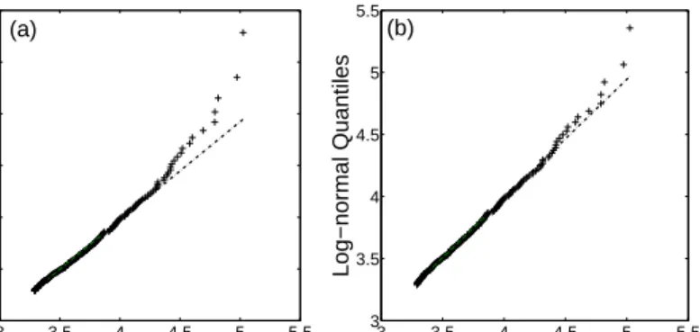
A visual comparison between the two hypotheses can be made by looking at the Quantile Quantile (QQ) plots for the empirical data compared to each of the two hypotheses. In a QQ-plot we plot the quantiles of one distribution as the x-axis and the other’s as the y-axis. If the two distributions are the same then we expect the points to fall on a straight line. Figure 2 compares the two hypotheses, making it clear that the log-normal is a much better fit than the power law. For the log-normal QQ plot most of the large values in the distribution fall on the dashed line corresponding to a log-normal distribution, though the very largest values are somewhat above the dashed line. This says that the empirical distribution decays slightly faster than a log-normal. There are two possible interpretations of this result: Either this is a statistical fluctuation or the true distribution really has slightly thinner tails than a log-normal. In any case, since a log-normal decays faster than a power law, it strongly suggests that the power law hypothesis is incorrect and the log-normal distribution is a better approximation.
A more quantitative method to address the question of which hypothesis better describes the data is to compare the likelihood of the observation in both hypotheses [Clauset et al., 2007]. We define the likelihood for the tail
v ariable 91 92 93 94 95 96 97 98 99 00 01 02 03 04 05 mean std R -0.50 -1.35 -1.49 -1.71 -3.29 -18.42 -2.25 -1.29 -6.57 -4.96 -2.63 -2.95 -2.00 -1.05 -0.99 -3.43 4.45 N 372 1069 1509 2194 2699 3300 4253 4885 5363 5914 6607 7102 7794 8457 8845 -E[ s ] (mn) 810 385 480 398 448 527 559 619 748 635 481 335 425 458 474 519 134 Std[ s ] (bn) 1.98 0.99 1.7 1.66 1.68 2.41 2.82 3.38 4.05 3.37 2.69 1.87 2.45 2.64 2.65 2.42 0.8 E[ ω ] 5.58 4.40 4.40 3.86 3.86 3.91 3.84 3.85 4.06 3.97 3.60 3.37 3.55 3.51 3.59 3.96 0.54 Std[ ω ] 1.51 1.98 2.09 2.43 2.50 2.46 2.50 2.51 2.46 2.45 2.63 2.42 2.49 2.59 2.50 2.34 0.29 ζs 1.33 1.36 1.19 1.15 1.11 0.78 1.08 1.10 0.95 0.97 1.01 1.07 1.07 1.10 1.14 1.09 0.14 smin 955 800 695 708 877 182 1494 1945 1147 903 728 836 868 1085 1383 974 408 Ntail 81 129 232 256 280 1067 290 283 557 662 717 494 652 630 550 -p -v alue 0.58 0.48 0.02 0.45 0.07 0 0.01 0.11 5 10 − 4 0.04 0.03 0.07 0.08 0.08 0.15 0.15 0.19 µ (10 − 3 ) 26 42 81 46 72 67 58 39 39 20 -3 -10 50 18 30.5 38.5 26 σ (10 − 1) 0.78 2.0 2.6 3.0 2.3 2.8 2.9 3.0 2.8 2.8 2.5 2.4 2.4 2.4 2.5 2.5 0.55 Nexit 0 41 45 61 139 115 169 269 308 482 427 660 703 675 626 -Nenter 185 338 581 783 759 885 1216 1342 1182 1363 1088 1063 1056 796 732 891 346 T able 1: T able of mon thly parameter v alues for equit y funds defined suc h that the p ortfolio con tains a fraction of at least 80% sto cks. The v alues for ea ch of the mon thly parameters (ro ws) w ere calculated for eac h y ear (columns). The mean and standard deviation ar e ev aluated for the mon thly v alues in eac h y ear. R -the base 10 log lik eliho o d ratio of a p o w er la w fit relativ e to a log-norma l fit as giv en b y equation (3) . A neg ativ e v alue of R indicates that the log-normal h yp othesis is a lik elier description than a p o w er la w. F or all y ears the v alue is negativ e meaning that the log-norm al distribution is more lik ely . N -the n um b er of equit y funds existing at the end of eac h y ear. E [ ω ] -the mean log size of funds existing at the end of eac h y ear. S td [ ω ] -the standard deviation of log sizes for funds existing at the end of eac h y ear. E [ s ] -the mean size (in millions) of funds existing at th e end of eac h y ear. S td [ s ] -the standard deviation of sizes (in bil lions) for funds existing at the end of eac h y ear. ζs -the p o w er la w tail exp onen t (1). smin -the lo w er tail cutoff (in millions of dollars) ab o v e whic h w e fit a p o w er la w (1 ). Ntail -the n um b er of equit y funds b elongin g to the u pp er tail s.t. s ≥ smin . p -v alue -the probabilit y of obtaining a go o dness of fit at least as bad as the one calculated for the empirical data, under the n ull h yp othesis of a p o w er la w upp er tail. µ -the drift term for the geometric random w alk (10), computed for mon thly changes. σ -the standard deviation of th e mean zero Wiener pro cess (10), co mputed for mon thly changes. Nexit -the n um b er of equit y funds exiting the industry eac h y ear. Nenter -the n um b er of new equit y funds en tering the industry in eac h y ear.
3 3.5 4 4.5 5 5.5 3 3.5 4 4.5 5 5.5 Empirical Quantiles Log−normal Quantiles 3 3.5 4 4.5 5 5.5 3 3.5 4 4.5 5 5.5 6 Empirical Quantiles
Power Law Quantiles
(a) (b)
Figure 2: A Quantile-Quantile (QQ) plot for the upper tail of the size distribution of equity funds. The quantiles are the base ten logarithm of the fund size, in millions of dollars. The empirical quantiles are calculated from the size distribution of funds existing at the end of the year 1998. The empirical data were truncated from below such that only funds with size
s ≥ smin were included in the calculation of the quantiles. (a) A QQ-plot
with the empirical quantiles as the x-axis and the quantiles for the best fit power law as the y-axis. The power law fit for the data was done using the maximum likelihood described in Section 3.1, yielding smin = 1945 and α = 1.107. (b) A QQ-plot with the empirical quantiles as the x-axis and the quantiles for the best fit log-normal as the y-axis, with the same smin as in
(a). The log-normal fit for the data was done used the maximum likelihood estimation given smin (2) yielding µ= 2.34 and σ= 2.5.
−80 −6 −4 −2 0 2 4 6 8 1 2 3 4 5
log−normal tail power law tail
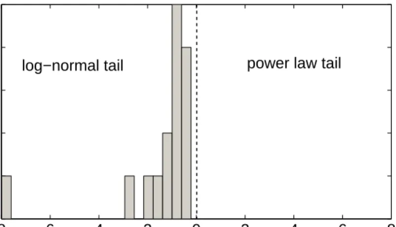
Figure 3: A histogram of the base 10 log likelihood ratiosRcomputed using (3) for each of the years 1991 to 2005. A negative log likelihood ratio implies that it is more likely that the empirical distribution is log-normal then a power law. The log likelihood ratio is negative in every year, in several cases strongly so.
of the distribution to be
L= Y
sj≥smin
p(sj).
We define the power law likelihood asLP L =Qsj≥sminpP L(sj) with the
prob-ability density of the power law tail given by (1). The lognormal likelihood is defined as LLN = Qsj≥sminpLN(sj) with the probability density of the
lognormal tail given by
pLN(s) = p(s) 1−P(smin) = √ 2 s√πσ " erfc lns√min−µ 2σ !#−1 exp " −(lns−µ) 2 2σ2 # . (2)
The more probable that the empirical sample is drawn from a given dis-tribution, the larger the likelihood for that set of observations. The ratio indicates which distribution the data are more likely drawn from. We define
the log likelihood ratio as R = ln L P L LLN . (3)
For each of the years 1991 to 2005 we computed the maximum likelihood estimators for both the power law fit and the log-normal fit to the tail, as explained above and in Section 3.1. Using the fit parameters, the log likelihood ratio was computed and the results are summarized graphically in Figure 3 and in Table 1. The ratio is always negative, indicating that the likelihood for the log-normal hypothesis is greater than that of the power law hypothesis in every year. It seems clear that tails of the mutual fund data are much better described by a log-normal than by a power law.
4
Empirical investigation of size dynamics
Our central thesis in this paper is that the mutual fund size distribution can be explained by a stochastic process governed by three key underlying processes: the size change of existing mutual funds, the entry of new funds and the exit of existing funds13. In this section we empirically investigate
each of these three processes, providing motivation for the model developed in the next section.
4.1
Fund entry process
We begin by examining the entry of new funds. We investigate both the number of funds entering each year Nenter(t) and the sizes with which they
enter. We perform a linear regression of Nenter(t) against the number of
existing funds N(t−1), yielding slope α = 0.04±0.05 and intercept β = 750±300. The slope is not statistically significant, and so we approximate fund entry as a Poisson process with a constant rate ν.
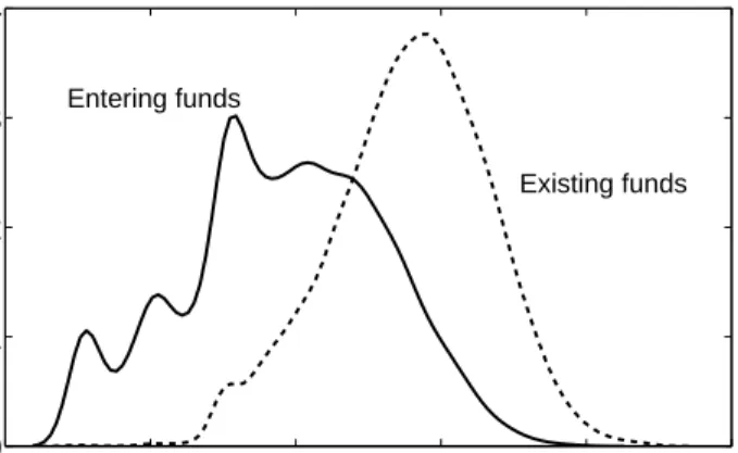
The size of entering funds is more complicated. In Figure 4 we compare the distribution of the size of entering fundsf(s) to that of all existing funds.
13In addition to the entry and exit processes, existing funds can merge or split. To
keep the model as simple as possible we include these in the entry and exit processes. For example, when two funds merge we treat this as two funds exiting the industry and another one entering. This greatly simplifies the model, and though it introduces some correlations, these are small enough that they can be safely neglected.
variable 1991- 1998 1991- 2005 ω0 0.14 −0.37 σω 3.02 3.16 σ0 0.35±0.02 0.30±0.02 β 0.31±0.03 0.27±0.02 σ∞ 0.05±0.01 0.05±0.01 µ0 0.15±0.01 0.08±0.05 α 0.48±0.03 0.52±0.04 µ∞ 0.002±0.008 0.004±0.001
Table 2: Model parameters as measured from the data in different time periods. ω0 and σ2ω are the mean and variance of the average (log) size of
new funds described in (4). σ0, β and σ∞ are the parameters for the size
dependent diffusion and µ0, α and µ∞ are the parameters of the average
growth rate (9). The confidence intervals are 95% under the assumption of standard errors. The time intervals were chosen to match the results shown in Fig. 9. −40 −2 0 2 4 6 0.1 0.2 0.3 0.4
log
10(s)
p(s)
Existing funds Entering fundsFigure 4: The probability density for the size s of entering funds in millions of dollars (solid line) compared to that of all funds (dashed line) including all data for the years 1991 to 2005. The densities were estimated using a gaussian kernel smoothing technique.
The distribution is somewhat irregular, with peaks at round figures such as ten thousand, a hundred thousand, and a million dollars. The average size14 of entering funds is almost three orders of magnitude smaller than that of existing funds, making it clear that the typical surviving fund grows significantly after it enters. We compared the distribution of entering funds to a log-normal and found that the tails are substantially thinner than those of the log-normal. When we consider these facts (small size and thin tails) it is clear that the distribution of entering funds cannot be important in determining the upper tail of the fund size distribution.
To conclude, the fund entry process is reasonably well approximated as a Poisson process in which an average of ν funds enter per month, with the size of each fund drawn from a distribution f(ω, t). The distribution of new fund sizes is approximated as a log-normal distribution in the fund size s, that is a normal distribution in the log size ω
f(ω, t) = q1 πσ2 ω exp −(ω−ω0) 2 σ2 ω ! θ(t−t0), (4)
where ω0 is the mean log size of new funds and σω2 is its variance. θ(t−t0)
is a unit step function ensuring no funds funds enter the industry before the initial time t0. The value of the mean log size and its variance are calculated
from the data for different periods, as summarized in Table 2.
4.2
Fund exit process
As we will show later, fund exit is of critical importance in determining the long-run properties of the fund size distribution. In Figure 5 we plot the number of exiting funds Nexit(t) as a function of the total number of funds
existing in the previous year, N(t−1). The linearly increasing trend is clear, and in most cases the number of exiting funds is within a standard deviation of the linear trend line. This suggests that it is a reasonable approximation to assume that the probability for a given fund to exit is independent of time,
14 When discussing the average size one must make sure to account for the difference
between the average log size and the average size, since due to the heavy tails the difference is striking. The average entry log size E[ωc]≈0, corresponding to a fund of size one million,
while if we average over the entry sizes E[sc] = E[eωc], we get an average entry size of
approximately 30 million. For comparison, both the average size and the average log size of existing funds are quoted in Table 1.
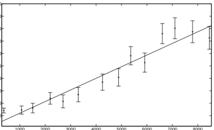
1000 2000 3000 4000 5000 6000 7000 8000 0 100 200 300 400 500 600 700 800 900 N(t−1) Nexit (t)
Figure 5: The number of equity funds exiting the industry Nexit(t) in the
year t as a function of the total number of funds existing in the previous year, N(t−1). The plot is compared to a linear regression (full line). The error bars are calculated for each bin under a Poisson process assumption, and correspond to the square root of the average number of funds exiting the industry in that year.
so that the number of exiting funds is proportional to the number of existing funds, with proportionality constant λ(ω), where ω is the logarithm of the fund size. Furthermore, it seems to be reasonable to assume thatλ(ω) =λis independent of size; where λis the slope of the linear regression in Figure 5. On an annual time scale this gives λ= 0.092±0.030. Under the assumption that fund death is a Poisson process the monthly rate is just the yearly rate divided by the number of months per year. Thus, we approximate the fund exit process as a Poisson process where funds of sizeω exit the industry with a constant rate λ.
4.3
Fund growth
Fund growth is a complicated process as it involves not only size changes due to fund performance but also changes due to investors depositing and withdrawing money. The investor behavior induces correlations and size dependence in the random process. It is convenient to define the relative
change in a fund’s size ∆s(t) as
∆s(t) =
s(t+ 1)−s(t)
s(t) . (5)
The relative change can be decomposed into two parts: the return ∆r and
the fractional investor money flux ∆f(t), which are simply related as
∆s(t) = ∆f(t) + ∆r(t). (6)
The return ∆r represents the return of the fund to its investors, defined as
∆r(t) =
N AV(t+ 1)−N AV(t)
N AV(t) , (7)
where N AV(t) is the Net Asset Value at timet. The fractional money flux ∆f(t) is the change in the fund size by investor deposits or withdrawals,
defined as
∆f(t) =
s(t+ 1)−[1 + ∆r(t)]s(t)
s(t) . (8)
Since the data set only contains information about the size of funds and their returns we are not able to separate deposits from withdrawals, but rather can only observe their net.
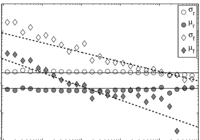
Figure 6 gives an overview of the size dependence for both the returns ∆r
and the money flux ∆f. The two behave very differently. The returns ∆r are
essentially independent of size15. This is expected based on market efficiency,
as otherwise one could obtain superior performance simply by investing in larger or smaller funds [Malkiel, 1995]. This implies that equity mutual funds can be viewed as a constant return to scale industry [Gabaix et al., 2006]. Both the mean µr =E[∆r] and the standard deviation σr = Var[∆r]1/2 are
constant; the latter is also expected from market efficiency, as otherwise it would be possible to lower one’s risk by simply investing in funds of a different size.
15The independence of the return ∆
ron size is verified by performing a linear regression
of µr vs. s for the year 2005, which results in an interceptβ = 6.7±0.2×10⁻³ and a
slopeα= 0.5±8.5×10⁻⁸. This result implies a size independent average monthly return
100 101 102 103 104 105 10−4 10−3 10−2 10−1 100 101 s σr µr σf µf
Figure 6: The average monthly returnµrand its volatilityσr, and the money
flux µf and its volatility σf, are plotted as a function of the fund size (in
millions) for the year 2005 (see Eqs. (5 - 8)). The data are binned based on size, using bins with exponentially increasing size. The average monthly returnµris compared to a constant return of 0.008 and the monthly volatility σr is compared to 0.03. The average monthly fluxµf is compared to a slope
of -0.5 and the money flux volatilityσf is compared to a linear slope of -0.35.
On a double logarithmic scale a line of slope α corresponds to a power law relation f(s) = sα.
In contrast, the money flow ∆f decreases with size. Both the mean money
fluxµf =E[∆f] and its standard deviationσf = Var[∆f]1/2 roughly follow a
power law over five orders of magnitude in the size s. This is similar to the behavior that has been observed for the growth rates of other types of firms [Stanley et al., 1995, 1996; Amaral et al., 1997a; Bottazzi and Secchi, 2003a]. Several theories have been put forth to explain this for firms in general, but at this point there is no consensus view as to its cause16. For mutual funds
one would expect that in absolute terms, all else being equal, it is harder to raise large amounts of money than small amounts of money, and thus the relative growth rate should decrease with size. This does not, however, explain why the functional form should be a power law. The fact that similar behavior is observed for other types of firms suggests that there should be a common explanation that holds for firms in general, and is not specific to mutual funds.
These two effects can be combined to model the mean total size changeµs
and the standard deviation σs. The standard deviations are related through
the approximate relation
σ2s ≈σf2+σr2.
This is only an approximation since we neglected the correlation term be-tween ∆r and ∆f. Based on our empirical studies the correlation is close to
zero and this is a good approximation. In Figure 7 we plot both µs and σs
as a function of size.
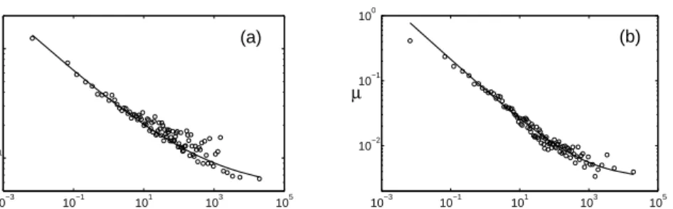
The decomposition illustrated in Figure 6 suggests thatµs andσs can be
reasonably well approximated as
σs(s) = σ0s−β+σ∞ (9)
µs(s) = µ0s−α+µ∞.
As illustrated in Figure 7, these functional forms fit the data reasonably well, with only slight variations of parameters in different periods, as shown in Table 2.
To summarize: In one respect, mutual funds are like other firms, in that their money flux shows the same power law decay with size that has been
16There has been a significant body of work attempting to explain the observed growth
rate of firms. For the main body of work see [Amaral et al., 1997b; Buldyrev et al., 1997; Amaral et al., 1998; De Fabritiis et al., 2003b; Matia et al., 2004; Bottazzi, 2001b; Sutton, 2001; Wyart and Bouchaud, 2002; Bottazzi and Secchi, 2003b, 2005b; Fu et al., 2005; Riccaboni et al., 2008; Podobnik et al., 2008].
10−3 10−1 101 103 105 10−1 100 s σ 10−3 10−1 101 103 105 10−2 10−1 100 s µ (a) (b)
Figure 7: (a) The standard deviationσ in the logarithmic size change ∆s=
∆(logs) of an equity fund as a function of the fund size s (in millions of dollars). (b) The meanµlogarithmic size change ∆s = ∆(logs) of an equity
fund as a function of the fund size s (in millions of dollars). The data for all the funds were divided into 100 equally occupied bins. µis the mean in each bin and σ is the square root of the variance in each bin for the years 1991 to 2005. The data are compared to a fit according to (9) in Figures (a) and (b) respectively.
observed for the growth rates of other firms. At the same time, mutual funds are unusual in that a component of their growth comes from the returns of the fund itself; this component is independent of size, as expected from market efficiency. Thus mutual funds are unusual in that, due to market efficiency, their relative growth rate does not go to zero in the limits→ ∞. The upshot is that for small funds money flux is the dominant growth process and for large funds the return is the dominant growth process. This means that for the largest funds we can approximate the mean and standard deviation of the growth rate as being size independent.
4.4
Diffusion model
We approximate the growth of existing funds as a multiplicative Gibrat-like process17 satisfying a stochastic evolution equation of the form
ds=s[µs(s)dt+σs(s)dWt], (10)
17A Gibrat-like process is a multiplicative process in which the size of the fund at any
given time is given as a multiplicative factor times the size of the fund at a previous time. In Gibrat’s law of proportionate effect [Gibrat, 1931] the multiplicative term depends linearly on size while here we allow it to have any size dependence.
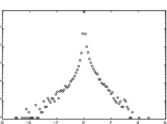
−6 −4 −2 0 2 4 6 10−6 10−5 10−4 10−3 10−2 10−1 100 ∆ω p( ∆ω )
Figure 8: The PDF of aggregated monthly log size changes ∆w = log10(1 + ∆s) for equity funds in the years 1991 to 2005. The log size
changes were binned into 20 bins for positive changes and 20 bins for neg-ative changes. Monthly size changes were normalized such that the average log size change in each month was zero.
where Wt is a mean zero and unit variance normal random variable, µs is
the drift and σs is the volatility. The use of an underlying Wiener process
in the stochastic evolution equation (10) assumes implicitly that the relative size change distributions of funds of a given size is an i.i.d normal random variable.
We first discuss the normality assumption. As can be seen in Figure 8, the relative size change distribution has a tent shape when plotted in semi-logarithmic scale18. It can be approximated as a double exponential, also called a Laplace distribution, which has heavier tails than a normal distri-bution. Nonetheless, due to the fact that the logarithmic increments are additive, after several steps the central limit theorem causes this to quickly converge to a normal distribution. We have explicitly verified this by track-ing a group of funds in a given size range over time. Thus even though the normality assumption is not true on short timescales it rapidly becomes valid on longer timescales.
The second approximation is that of an independent process. Strictly speaking this approximation is also violated, due to the fact that investors
18 A similar phenomenon was originally observed by Stanley et al for the distribution
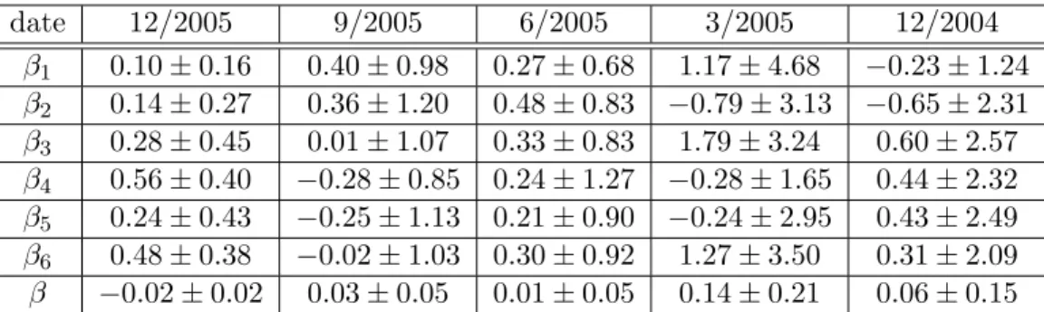
date 12/2005 9/2005 6/2005 3/2005 12/2004 β1 0.10±0.16 0.40±0.98 0.27±0.68 1.17±4.68 −0.23±1.24 β2 0.14±0.27 0.36±1.20 0.48±0.83 −0.79±3.13 −0.65±2.31 β3 0.28±0.45 0.01±1.07 0.33±0.83 1.79±3.24 0.60±2.57 β4 0.56±0.40 −0.28±0.85 0.24±1.27 −0.28±1.65 0.44±2.32 β5 0.24±0.43 −0.25±1.13 0.21±0.90 −0.24±2.95 0.43±2.49 β6 0.48±0.38 −0.02±1.03 0.30±0.92 1.27±3.50 0.31±2.09 β −0.02±0.02 0.03±0.05 0.01±0.05 0.14±0.21 0.06±0.15
Table 3: Cross-sectional regression coefficients of the monthly fund flow, computed for several months, against the performance in past months, as indicated in Eq. 11. The regression was computed cross-sectionally using data for 6189 equity funds. For example the entry for β1 in the first (from
the left) column represents the linear regression coefficient of the money flux at the end of 2005 on the previous month’s return. The errors correspond to the 95% confidence intervals.
react to past performance19. This causes correlations in the money flux ∆
f,
which in turns induces correlations in the total size change ∆s. We find,
however, that these correlations are small. This can be seen in Table 3. We perform cross sectional regressions for several different times t of the form
∆f(t) = β+β1∆r(t−1) +β2∆r(t−2) +. . .+β6∆r(t−6). (11)
The results are extremely noisy; for example, eight of the thirty possible coefficients βi are negative and only two of them are significant at the two
standard deviation level. The independent process approximation is partic-ularly true for large funds where the size growth is dominated by the return ∆r, which is essentially uncorrelated due to market efficiency [Bollen and
Busse, 2005; Carhart, 1997].
19For empirical evidence that investors react to past performance see [Remolona et al.,
1997; Busse, 2001; Chevalier, Judith and Ellison, Glenn, 1997; Sirri, Erik R. and Tufano, Peter, 1998; Guercio, Diane Del and Tkac, Paula A., 2002; Bollen, 2007].
5
An analytical model for the mutual fund
size distribution
The empirical evidence described in the previous section motivates a simple stochastic growth model for the equity mutual fund industry. The aim of the model is to describe the time evolution of the size distribution, that is, to solve for the probability density function p(ω, t) of funds with (log) size ω
existing at time t. The size distribution can be written as
p(ω, t) = n(ω, t)
N(t) , (12)
where n(ω, t) is the number of funds at time with logarithmic size ω and
N(t) = R
n(ω, t)dω is the total number of funds at time t. To simplify the analysis we solve separately for the total number of funds N(t) and for the number density n(ω, t).
5.1
Dynamics of the total number of funds
Based on the empirical observations of Section 4, we have argued that it is natural to model the total number of funds as a function of time as
dN
dt =ν−λN (13)
where ν is the rate of creating new funds and λ is the exit rate of exist-ing funds. Under the assumption that ν and λ are constant in time and independent of N this has the solution
N(t) = ν
λ
1−e−λtθ(t), (14) where θ(t) is a unit step function at t = 0, the year in which the first funds enter. This solution has the surprising property that the dynamics only depend on the fund exit rate λ, with a characteristic timescale 1/λ. For example, for λ ≈ 0.09, as estimated in Section 4, the timescale for N(t) to reach its steady state is only roughly a decade. An examination of Table 1 makes it clear, however, thatν = constant is not a very good approximation. Nonetheless, if we crudely use the mean creation rate ν ≈900 from Table 1 and the fund exit rate λ ≈ 0.09 estimated in Section 4, the steady state
number of funds should be about N ≈10,000, compared to the 8,845 funds that actually existed in 2005. Thus this gives an estimate with the right order of magnitude.
The important point to stress is that the dynamics forN(t) operate on a different timescale than that of n(ω, t). As we will show in the next section the characteristic timescale for n(ω, t) is much longer than that forN(t).
5.2
Analytical solution for the number density
n
(
ω, t
)
We define and solve the time evolution equation for the number density
n(ω, t) using the empirically motivated approximations described earlier. These approximations are: The entry process is modeled as a Poisson pro-cess with rate ν, such that at time t a new fund enters the industry with a probabilityνdtand (log) sizeω drawn from a distributionf(ω, t). The entry size distribution is approximated as normal distribution in log size given by equation (4). The exit process is modeled as an individual Poisson process such that at any time time t a fund exits the industry with a size indepen-dent probability λdt. The size change is approximated as a (log) Brownian motion with a size dependent drift and diffusion term given by equation (9). Under these assumptions the forward Kolmogorov equation (also known as the Fokker-Plank equation) defining the time evolution of the number density [Gardiner, 2004] is given by ∂ ∂tn(ω, t) =νf(ω, t)−λn(ω, t)− ∂ ∂ω[µ(ω)n(ω, t)] + ∂2 ∂ω2[D(ω)n(ω, t)], (15)
where D(ω) = σ(ω)2/2 is the size diffusion coefficient. The first term on the right describes the entry process, the second describes the fund exit process and the third and fourth terms describe the change in size of an existing fund. Under the change of variables s = exp(ω) in (9) the size dependent drift and diffusion terms are given by
µ(ω) = µ0e−αω+µ∞ (16)
σ(ω) = σ0e−βω+σ∞.
5.2.1 Approximate solution for large funds
Eqs. (15) and (16) cannot be solved analytically, but a great deal of insight can be gained by going to the large size limit. As previously described, due
to the dominance of the returns, in this limit ∆s ≈ ∆r, and µ(ω) and σ(ω)
are constant, i.e. µ=µ∞ and σ=σ∞. The evolution equation becomes ∂ ∂tn(ω, t) = νf(ω, t)−λn(ω, t)−µ ∂ ∂ωn(ω, t) +D ∂2 ∂ω2n(ω, t), (17)
where we used the notation D = σ∞2 /2. The upper tail behavior of the
distribution described by (17) strongly depends on the exit and entry process. If for example, funds only change in size and no funds enter or exit, then the resulting distribution is normal
˜ n(w, t) = √ 1 4πDtexp " −(ω−µt) 2 4Dt # , (18)
which corresponds to a size distribution p(s) with a lognormal upper tail. The exit process plays a major role and is responsible for the thickening with time of the upper tail of the distribution. The intuition is as follows: Since each fund exits the industry with the same probability and since there are more smaller sized funds than larger ones the number of small funds exiting the industry is larger. This results in an increasing fraction of larger funds. As we will now show this results in the distribution evolving from a log-normal upper tail to a power law upper tail. In contrast, the entry process is not as important and determines mainly the number of funds in the industry. This is true as long as the entry size distribution f(ω, t) is not heavier-tailed than a lognormal, which is supported by the empirical data.
In the large size limit the solution for an arbitrary entry size distribution
f is given by n(ω, t) = ν Z ∞ −∞ Z t 0 exp−λt0 √ 1 4πDt0exp " −(ω−ω 0−µt)2 4Dt0 # f(ω0, t−t0) dt0dω0. (19) Stated in words, a fund of size ω0 enters at time t − τ with probability
f(ω0, t−τ). The fund will survive to time t with a probability exp(λτ) and will have a size ω at time t with a probability according to (18).
If funds enter the industry with a constant rateνbeginning att = 0, with a log-normal entry size distributionf(ω, t) centered around ωswith widthσs
as given by (4), the size density can be shown to be
n(ω, t) = νµ 4√γDexp " (γ+1 4) σs2 2 − √ γ σs2 2 + µ D(ω−ωs) + µ 2D(ω−ωs) # × A+ exp √ γ|σs2+ 2µ D(ω−ωs)| B , (20)
where the drift and diffusion terms are approximated as µ = µ∞ and D = σ∞2 /2. The parameters A, B and γ are defined as
γ = s 1 4 + λD µ2 , (21) A = Erf σ2 s 2 + µ D(ω−ωs) − √ γσ2 s √ 2σs − Erf σ2 s 2 + µ D(ω−ωs) − √ γσ2 s + 2 µ2 Dt √ 2qσ2 s+ 2 µ2 Dt (22) and B = Erf √ γσs2 2 + µ2 Dt +|σ2s 2 + µ D(ω−ωs)| √ 2qσ2 s + 2 µ2 Dt −Erf √ γσ2s+ σ2 s 2 + µ D (ω−ωs) √ 2σs , (23) where Erf is the error function, i.e. the integral of the normal distribution.
5.2.2 Steady state solution for large funds
Making a further approximation simplifies the solution considerably. Let us define a large fund as one with ω ωs, where ωs is the logarithm of the
typical entry size of one million USD. For large funds we can approximate the lognormal distribution as having zero width, in other words we assume that all new funds have the same size ωs. The number density is then given
by n(ω, t) = νD 4√γµ2e 1 2 µ D(ω−ωs) " e−√γDµ|ω−ωs| 1 + erf s γµ2t D − |ω−ωs| 2√Dt − e√γDµ|ω−ωs| 1−erf µ s t D( 1 2+ √ γ) # ,
where we have approximated the drift and diffusion as µ = µ∞ and D = σ2
∞/2. Since γ > 1/4 (21), the density vanishes for both ω → ∞ and
The steady state solution for large times is achieved by taking thet→ ∞
limit of (24), which gives
n(ω) = ν 2µ√γ exp µ D ω−ω s 2 − √ γ|ω−ωs| . (24)
Since the log size density (24) has an exponential upper tailp(ω)∼exp(−ζsω)
and s = exp(ω) the CDF for s has a power law tail with an exponent20 ζ
s,
i.e.
P(s > X)∼X−ζs. (25)
Substituting for the parameter γ using Eq. (21) for the upper tail exponent yields
ζs =
−µ+√µ2+ 4Dλ
2D . (26)
Note that this does not depend on the creation rate ν. Using the average parameter values in Table 2 the asymptotic exponent has the value
ζs= 1.2±0.6. (27)
This suggests that when the distribution will reach its steady state the tails will be in agreement with those expected under Zipf’s law, ζs ≈1.
5.2.3 The importance of µ∞ and σ∞
The non vanishing drift µ∞ > 0 and diffusion terms σ∞ > 0 are essential
for the distribution to evolve towards a power law. As can be seen from the fit parameters, based on data for ∆s alone, we cannot strongly reject the
hypothesis that the drift and diffusion rates vanish for large sizes, i.e. µ∞→0
and σ∞→0. However, because the size change ∆s can be decomposed into
∆rand ∆f, and because the mean of ∆r >0 due to the growth of the market,
we are confident that neither µ∞ nor σ∞ are zero.
This distinguishes mutual funds from other types of firms, which are typically observed empirically to have σ∞ = 0 [Stanley et al., 1996; Matia
et al., 2004]. It suggests that in a sufficiently stationary situation and after the passage of sufficient time their distributions should be different. Previous empirical studies for other firms found µ∞ = 0 and σ∞ = 0. Assuming that
20 To calculate the tail exponent of the density correctly one must change variables
throughp(s) =p(ω)ddωs ∼s−ζs−1. This results in a CDF with a tail exponent ofζ
other types of firms obey similar diffusion equations to those used here, it can be shown that the resulting distribution has a stretched exponential upper tail, which is much thinner than a power law21.
5.2.4 Timescale to reach steady state
The most useful aspect of solving for the time dependent solution is that it provides the ability to estimate the timescale to reach the steady state solution. The time dependence in Eq. 24 is contained in the arguments of the error function terms on the right. When these arguments become large, say larger than 3, the solution is roughly time independent, and can be written as t > 9D 4γµ2 1 + s 1 + 2 9 √ γµ2 D |ω−ωs| 2 . (28)
Using the values obtained by fitting the whole data set, in units of months
µ=µ∞≈0.005, D=σ2∞/2 and σ∞≈0.05. This gives t >180 1 + q 1 + 0.7|ω−ωs| 2 ,
where the time is in months. Plugging in some numbers makes it clear that the time scale to reach steady state is very long. For instance, for funds of a billion dollars it will take about 170 years for their distribution to come within 1 percent of its steady state. This agrees with the observation that there seems to be no significant fattening of the tail over nearly two decades since 1991. Note that the time required for the distribution n(ω, t) to reach steady state for large values of ω is much greater than that for the total number of funds N(t) to become constant.
5.3
Comparisons to empirical data
We are unable to find an analytic solution for the general case of Eq. (15) including the size dependence of the diffusion and drift terms, and so we
21A stretched exponential is of the formp(x)∼exp(ax−b), whereaandb are positive
constants. There is some evidence in the empirical data that the death rateλalso decays with size. However, in our simulations we found that this makes very little difference for the size distribution as long as it decays slower than the distribution of entering funds, and so in the interest of keeping the model parsimonious we have not included this in our model.
employ a simulation. This was done on a monthly time scale, averaging over 1000 different runs to estimate the final distribution. As we have emphasized in the previous discussion the time scales for relaxation to the steady state distribution are long. We thus take the evidence for the huge increase in the number of new funds seriously. We begin the simulation in 1991 and simulate the process for varying periods of time, making our target the empirical data at the end of the period. In each case we assume the size distribution for injecting funds is log-normal, as discussed in Section 4.1.
To compare our predictions to the empirical data we measure the pa-rameters for each of the processes of fund creation, entry and exit using data from the same period as the simulation, summarized in Table 2. A key point is that we are not fitting these parameters on the target data for fund size22, but rather are fitting them on the individual creation, exit and
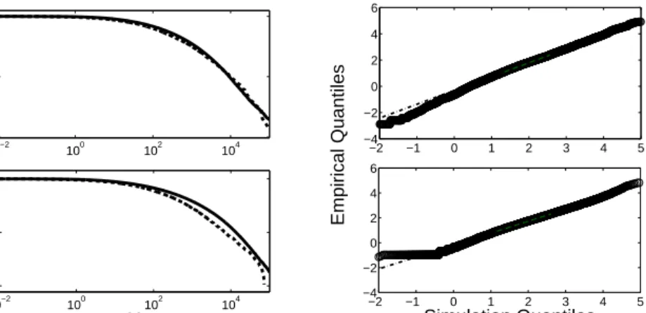
diffusion processes and then simulating the corresponding model to predict fund size. One of our main predictions is that the time dependence of the solution is important. In Figure 9 we compare the predictions of the simula-tion to the empirical data at two different ending times. The model fits quite well at all time horizons, though the fit in the tail is somewhat less good at the longest time horizon. This indicates that even for this model there is a slight tendency to estimate a tail that is heavier than that of the data. Note, however, that the simulations also make it clear that the fluctuations in the tail are substantial, and this deviation is very likely due to chance – many of the individual runs of the simulation deviate from the mean of the 1000 simulations much more than the empirical data does.
6
Comparison with the hypothesis of Berk
and Green
As mentioned in the introduction, Berk and Green [2004] have offered an alternative hypothesis to ours, based on the distribution of fund manager skill and the size dependence of transaction cost. Under market efficiency the after-transaction returns of funds should be independent of size. Transaction
22 It is not our intention to claim that the processes describing fund size are constant
or even stationary. Thus, we would not necessarily expect that parameters measured on periods outside of the sample period will be a good approximation for those in the sample period. Rather, our purpose is to show that these processes can explain the distribution of fund sizes.
10−2 100 102 104 100 10−2 10−4 −2 −1 0 1 2 3 4 5 −4 −2 0 2 4 6 10−2 100 102 104 100 10−2 10−4 X P(s>X) −2 −1 0 1 2 3 4 5 −4 −2 0 2 4 6 Simulation Quantiles Empirical Quantiles
Figure 9: The model is compared to the empirical distribution at different time horizons. The left column compares CDFs from the simulation (full line) to the empirical data (dashed line). The right column is a QQ-plot comparing the two distributions. In each case the simulation begins in 1991 and is based on the parameters in Table 2. The first row corresponds to the years 1991-1998 and the second row to the years 1991-2005 (in each case we use the data at the end of the quoted year).
costs are known to increase with trading size. Thus, they argue, the difference between a large fund and small fund is that larger funds have higher before-transaction cost returns, corresponding to superior skill. This skill allows the funds to grow larger and make better profits by collecting more fees.
Given a distribution P(α) of investor skill α and a functional form g(s) for transaction costs, the Berk and Green model makes a prediction about the distribution of fund sizes. Berk and Green somewhat arbitrarily assumed thatP(α) is normal and thatg(s) is linear. This implies a normal distribution of fund size, which is clearly very different than what is observed. A more realistic assumption for transaction costs would be23 g(s)∼sb, withb ≈0.5.
Under this assumption it is possible to show that P(α) must have a log-normal upper tail in order to be consistent with the data. (This is true for anyb >0 including the Berk and Green choice ofb = 1). Whether or not this is plausible is not clear; certainly it means that the distribution of skill must be very heavy tailed. What is clear is that their theory has little predictive value for fund size as it stands, since the prediction of fund size is itself based on an unknown distribution for skill, which requires as much information to specify as the prediction itself.
In contrast, the prediction made by our hypothesis is very robust. While getting a good fit to the true fund size distribution requires several assump-tions, as we have spelled out here, under our model the log-normal upper tail depends only on the fact that returns are essentially random, and that the timescales to achieve the asymptotic distribution are extremely long. The essence of the answer emerges from the simple fact that returns are multi-plicative.
This brings up the question of whether or not our theory can be com-patible with the Berk and Green hypothesis. In our theory the aspect that transaction costs might affect is the mean inflow of money to funds as a func-tion of size, µf(s). This is where investor choice might enter our model. For
example, one can hypothesize that the net rate of deposits to larger funds decreases with size due to the fact that investors correctly understand that there are increased transaction costs. Alternatively, fund managers may un-derstand that they have higher costs and close their funds or take less relative effort in marketing them as they get bigger24.
23For a select body of work on the functional form of transaction cost see [Torre, 1997;
Kempf and Korn, 1999; Farmer and Lillo, 2004; Gabaix et al., 2003; Gabaix et al., 2006; Hopman, 2007; Bouchaud et al., 2008] and references therein.
While both of these effects are plausible, they do not qualitatively change the results of our model. The lognormal upper tail is very robust under variations of the investor money flux – the upper tail of the distribution is essentially independent of µf(s) and σf(s), as long as they stay within
reasonable bounds25. Thus, it seems that the diffusive nature of fund size
dominates investor choice in determining the fund size distribution.
We are in the process of making a more detailed study quantitatively testing the Berk and Green hypothesis, under several additional criteria that we do not have the space to explain here. We believe, though, that the data presented here already strongly suggest that their hypothesis cannot provide the correct explanation for fund size, while ours does.
7
Conclusions
In this paper we have shown that the empirical evidence strongly favors the hypothesis that the upper tail of the distribution of fund size is not a power law and is better approximated by a log-normal. Even though the log-normal distribution is strongly right skewed, and thus in some respects is a heavy-tailed distribution, it is still much thinner-tailed than a power law, as evidenced by the fact that all its moments exist. As a consequence there are fewer extremely large funds than one would expect if it were a power law. We have argued that the mutual fund size distribution is naturally ex-plained in terms of the stochastic nature of the growth process. The essential elements of the growth process are multiplicative random changes in the size of existing funds, entry of new funds, and exit of existing funds as they go out of business. We find, however, that entry plays no role at all other than setting the scale; exit plays a role in thickening the tails of the distribution, but this acts only on a very slow timescale. The log-normality comes about because the industry is young and still in a transient state. In the future, if the conditions for fund growth and removal remain stationary for more than a century, the distribution should become a power law. The thickening of the tails happens from the body of the distribution outward, as the power
the rate is increasing, so perhaps what one needs to explain is why there is an increase with fund size.
25The requirement is thatµ
s(s) remain greater than zero. It fails if eitherµf(s) orσ(s)
increases with size, which seems implausible, of ifµf(s) becomes sufficiently negative that
law tail extends to successively larger funds.
There is also an interesting size dependence in the growth rate of mutual fund size, which is both like and unlike that of other types of firms. Mutual funds are distinctive in that their overall growth rates can be decomposed as a sum of two terms, ∆s = ∆f + ∆r, where ∆f represents the flow of money
in and out of funds, and ∆r the returns on money that is already in the
fund. The money flow ∆f decreases as a power law as a function of size,
similar to what is widely observed in the overall growth rates for other types of firms. Furthermore the exponents are similar to those observed elsewhere. The returns ∆r, in contrast, are essentially independent of fund size, as they
must be under market efficiency. As a result, for large sizes the mean and variance of the overall growth are constant – this is unlike other firms, for which the mean and variance appear to go to zero in the limit. As we discuss here, this makes an important difference in the long-term evolution: While mutual funds should eventually evolve toward a power law, other firms should evolve toward a thinner-tailed, stretched exponential distribution.
Our analysis here suggests that investor preference has a negligible influ-ence on the upper tail of the mutual fund size distribution. Investor prefer-ence enters our analysis only through ∆f, the flow of money in and out of
the fund. Since ∆f becomes relatively small in the large size limit, in this
limit the growth of funds is dominated by the returns ∆r, whose mean and
variance are constant. Thus the upper tail of the size distribution is deter-mined by market efficiency, which dictates both that returns are essentially random, and thus diffusive, and that there is no dependence on size. Thus for large fund size investor preference doesn’t have much influence on the growth process; this is reinforced by the fact that the statistical properties of the money flux ∆f are essentially like those of the growth of other firms.
This, as well as other arguments presented in the previous section, indicates that transaction costs do not play a major role in determining fund size, as suggested by Berk and Green (2004).
Our results present a puzzle as to what determines the distribution of trading volume. The existence of a power law for large trading volumes is now fairly well documented26. A possible explanation for the volume distri-bution assumes that fund trading is proportional to its size and relies on the
26For work arguing for a power law volume distribution see [Gopikrishnan et al., 2000;
Gabaix et al., 2003; Lillo et al., 2005; Gabaix et al., 2006], while Eisler and Kertesz [2006] argue against one.
assumption that funds size is described by a power law obeying Zipf’s law. Our analysis here shows that this argument fails for two reasons: (1) Mutual funds sizes do not follow Zipf’s law, and are not even power law distributed and (2) transaction costs are not important in determining fund size. Thus the puzzle of what determines the distribution of trading volume remains an open question.
We have argued here that the cause of the log-normal upper tail of the mutual fund size distribution is essentially market efficiency, combined with the fact that fund growth is a slow-moving, diffusive process that takes place on time scales measured in decades. Investors are not making rational allo-cations as posited by Berk and Green; rather they move their money in and out of funds slowly, and with a great deal of inertia. This explanation might be disappointing to some as having“little economic content”; its strength is that it explains an important economic phenomenon in a manner that is very robust, and largely independent of the details of human choice.
Acknowledgements
We would like to thank Brad Barder, Giovani Dosi, Fabrizio Lilo, Terry Odean, Eric Smith and especially Rob Axtell for useful comments. YS would like to thank Mark B. Wise for his support. We gratefully acknowledge financial support from Barclays Bank, Bill Miller and NSF grant HSD-0624351. Any opinions, findings and conclusions or recommendations expressed in this material are those of the authors and do not necessarily reflect the views of the National Science Foundation.
A
Simulation model
We simulate a model with three independent stochastic processes. These processes are modeled as Poisson process and as such are modeled as having at each time step a probability for an event to occur. The simulation uses asynchronous updating to mimic continuous time. At each simulation time step we perform one of three events with an appropriate probability. These probabilities will determine the rates in which that process occurs. The probability ratio between any pair of events should be equal to the ratio of the rates of the corresponding processes. Thus, if we want to simulate this model for given rates our probabilities are determined.
These processes we simulate are:
1. The rate of size change taken to be 1 for each fund andN for the entire population.
Thus, each fund changes size with a rate taken to be unity. 2. The fund exit rateλ which can depend on the fund size. 3. The rate of creation of new fundsν.
Each new fund enters with a size ω with a probability density f(ω). Since some of these processes are defined per firm as opposed to the creation process, the simulation is not straightforward. We offer a brief description of our simulation procedure.
1. At every simulation time step, with a probability 1+λν+ν a new fund enters and we proceed to the next simulation time step.
2. If a fund did not enter then the following is repeated (1 +λ)N times.
a. We pick a fund at random.
b . With a probability of 1+λλ the fund enters.
c. If it is not annihilated, which happens with a probability of 1+1λ, we change the fund size.
We are interested in comparing the simulations to both numerical and empirical results. The comparisons with analytical results are done for spe-cific times and for spespe-cific years when comparing to empirical data. In order to do so, we need to convert simulation time to ”real” time. The simulation
time can be compared to ’real’ time if every time a fund does not enter we add a time step. Because of the way we defined the probabilities each simula-tion time step is comparable to 1/(1 +λ) in ”real” time units. The resulting ”real” time is then measured in what ever units our rates were measured in. In our simulation we use monthly rates and as such a unit time step corresponds to one month.
References
Amaral, L. A. N., Buldyrev, S. V., Havlin, S., Maass, P., Salinger, M. A., Stanley, H. E., and Stanley, M. H. R. (1997a). Scaling behavior in eco-nomics: The problem of quantifying company growth.Physica A, 244:1–24. Amaral, L. A. N., Buldyrev, S. V., Havlin, S., Maass, P., Salinger, M. A., Stanley, H. E., and Stanley, M. H. R. (1997b). Scaling behavior in eco-nomics: The problem of quantifying company growth.Physica A, 244:1–24. Amaral, L. A. N., Buldyrev, S. V., Havlin, S., Salinger, M. A., and Stanley, H. E. (1998). Power law scaling for a system of interacting units with complex internal structure. Phys. Rev. Lett., 80(7):1385–1388.
Axtell, R. L. (2001). Zipf distribution of U.S. firm sizes. Science, 293(5536):1818–1820.
Berk, J. B. and Green, R. C. (2004). Mutual fund flows and performance in rational markets. Journal of Political Economy, 112(6):1269–1295.
Bollen, N. P. (2007). Mutual fund attributes and investor behavior. Journal
of Financial and Quantitative Analysis, 42(3):683–708.
Bollen, N. P. B. and Busse, J. A. (2005). Short-Term Persistence in Mutual Fund Performance. Rev. Financ. Stud., 18(2):569–597.
Bottazzi, G. (2001a). Firm diversification and the law of proportionate effect. Bottazzi, G. (2001b). Firm diversification and the law of proportionate effect. Bottazzi, G. and Secchi, A. (2003a). Common properties and sectoral speci-ficities in the dynamics of U.S. manufacturing companies. Review of In-dustrial Organization, 23(3-4).