Distribution of the Ratio of Normal and Rice Random Variables

Volume 12 | Issue 2 Article 27

11-1-2013

Distribution of the Ratio of Normal and Rice

Random Variables

Nayereh B. Khoolenjani

University of Isfahan, Isfahan, Iran, [email protected] Kavoos Khorshidian

Shiraz University, Shiraz, Iran

Follow this and additional works at:http://digitalcommons.wayne.edu/jmasm

Recommended Citation

Khoolenjani, Nayereh B. and Khorshidian, Kavoos (2013) "Distribution of the Ratio of Normal and Rice Random Variables,"Journal of Modern Applied Statistical Methods: Vol. 12: Iss. 2, Article 27.

Emerging Scholars:

Distribution of the Ratio of Normal and Rice

Random Variables

The ratio of independent random variables arises in many applied problems. The distribution of the ratio X

Y is studied when X and Y are independent Normal and Rice random variables, respectively. Ratios of such random variables have extensive applications in the analysis of noises in communication systems. The exact forms of probability density function (PDF), cumulative distribution function (CDF) and the existing moments are derived in terms of several special functions. As a special case, the PDF and CDF of the ratio of independent standard Normal and Rayleigh random variables have been obtained. Tabulations of associated percentage points and a computer program for generating tabulations are also given.

Keywords: Normal distribution, Rice distribution, ratio random variable, special functions.

Introduction

For given random variables X and Y, the distribution of the ratio X

Y arises in

a wide range of natural phenomena of interest, such as in engineering, hydrology, medicine, number theory, psychology, etc. More specifically, Mendelian inheritance ratios in genetics, mass to energy ratios in nuclear physics, target to control precipitation in meteorology, inventory ratios in economics are exactly of this type. The distribution of the ratio random variables (RRV) has been

extensively investigated by many authors especially when X and Y are

independent and belong to the same family. Various methods have been compared

and reviewed by authors including Pearson (1910), Greay (1930), Marsaglia

The exact distribution of X

Y is derived when X and Yare independent

random variables (RVs) having Normal and Rice distributions with parameters

2

( ,µ σ ) and ( , )λ v , respectively. The Normal and Rice distributions are well known and of common use in engineering, especially in signal processing and communication theory. In engineering, there are many real situations where measurements could be modeled by Normal and Rice distributions. Some typical situations in which the ratio of Normal and Rice random variables appear are as follows. In the case that X and Yrepresent the random noises corresponding to two signals, studying the distribution of the quotient X

Y is of interest. For

example in communication theory it may represent the relative strength of two different signals and in MRI, it may represent the quality of images. Moreover, because of the important concept of moments of RVs as magnitude of power and energy in physical and engineering sciences, the possible moments of the ratio of Normal and Rice random variables have been also obtained. Applications of Normal and Rice distributions and the ratio RVs may be found in Rice (1974), Helstrom (1997), Karagiannidis and Kotsopoulos (2001), Salo, et al. (2006), Withers and Nadarajah (2008) and references therein.

The probability density function (PDF) of a two-parameter Normal random variable X can be written as:

2 2 1 1 ( ) exp{ ( ) }, 2 2 X f x x µ x σ πσ = − − − ∞ < < ∞ (1)

where −∞ < < ∞µ is the location parameter and σ >0 is the scale parameter. For 0

µ = and 2

1

σ = , (1) becomes the distribution of standard Normal random

variable. A well known representation for CDF of X is as

1 ( ) 1 ( ) 2 2 X x F x erf µ σ −   = _ + _   (2)

where erf( )⋅ denotes the error function that is given by

2 2 ( ) x u erf x e du π − =

∫

Also, 2 2 2 0 1 ( ) ! ( ) . ( 2 )! ! 2 k k k j j E X k k j j σ µ µ       = = ⋅ −

∑

If Y has a Rice distribution with parameters ( , )λ v , then the PDF of Y is as follows: 2 2 0 2 2 2 ( ) ( ) exp{ } ( ), 0, 0, 0 2 Y y y v yv f y y v λ λ λ λ + = − Ι > ≥ > (5)

where y is the signal amplitude, Ι₀(.) is the modified Bessel function of the first kind of order 0, 2λ2 is the average fading-scatter component and v2 is the line-of-sight (LOS) power component. The Local Mean Power is defined as

2 2

2λ v

Ω = + which equals 2

( )

E X , and the Rice factor K of the envelope is

defined as the ratio of the signal power to the scattered power, i.e., 2 2

2

K =v λ . When K goes to zero, the channel statistic follows Rayleigh distribution, whereas if Kgoes to infinity, the channel becomes a non-fading channel. For v=0, the

expression (5) reduces to a Rayleigh distribution.

Notations and Preliminaries

Recall some special mathematical functions, these will be used repeatedly throughout this study. The modified Bessel function of first kind of order v, is

2 0 1 ( ) 1 ₄ ( ) ( ) 2 ( !) ( 1) k v v k x I x x k v k ∞ = = Γ + +

∑

The generalized hypergeometric function is denoted by

1 2 1 2 1 2 0 1 2 ( ) ( ) ...( ) ( , ,..., ; , ,..., ; ) ( ) ( ) ...( ) ! k k k p k p q p q k k k q k a a a z F a a a b b b z b b b k ∞ = =

∑

The Gauss hypergeometric function and the Kummer confluent hypergeometric function are given, respectively, by

2 1 0 ( ) ( ) ( , ; ; ) ( ) ! k k k k k a b z F a b c z c k ∞ = =

∑

∑

where ( )a _k, ( )b _k represent Pochhammer’s symbol given by

( ) ( ) ( 1) ( 1) ( ) k k a a a a k α α Γ + = + ⋅⋅⋅ + − = Γ .

The parabolic cylinder function is

2 2 2 4 1 1 1 ( ) 2 ( , ; ) 2 2 2 v z v D z = e− Ψ − v z (10)

where Ψ( , ; )a c z represents the confluent hypergeometric function given by

1 1 1 1 1 1 1 ( , ; ) ( ; ; ) 2 (1 ; 2 ; ) 1 c c c a c z F a c z F a c c z a c a − − −     Ψ = Γ_{ } + Γ_{ } + − − + −     , in which 1 1 1 1 ( ) ,..., ,..., ( ) m i m i n n j j a a a b b b = = Γ   Γ_{ }=   _Γ

∏

∏

2 2 ( ) u x erfc x e du π ∞ − =

_∫

The following lemmas are of frequent use.

Lemma 1 (Equation (2.15.5.4), Prudnikov, et al., 1986). For Rep>0 , Re(α+ >v) 0; argc <π 2 1 0 ( ) 2 1 2 1 1 ( ) ( ) 2 2 ( ; 1; ) 2 4 1 px v v v v x e I cx dx v v c c p F v p v α α α _α ∞ − − + − − − +   ₊   = Γ +   +  

∫

Lemma 2 (Equation (2.8.9.2), Prudnikov, et al., 1986). For Rep>0; arg 4 c <π 2 2 1 1 0 2 2 2 2 ( ) 0 ! ( 1) ( 1 2 2 1 ( ) exp( ) ( ) . n n px n n n erf cx b n x e dx erfc cx b p c pb bc erf b erfc P p _{p c p} c p _{c p} ∞ + − + +   ₌  _± −  ₊          ∂ _{+ −}   ∂ _{ +} + _{+ }

∫

Lemma 3 (Equation (3.462.1), Gradshteyn & Ryzhik, 2000). For Reβ >0 , Rev>0

{

}

∫

The Ratio of Normal and Rice Random Variables

The explicit expressions for the PDF and CDF of X Y are derived in terms of the Gauss hypergeometric function. The ratio of standard Normal and Rayleigh RVs is also considered as a special case.

Theorem 1: Suppose that X and Y are independent Normal and Rice random variables with parameters ( ,µ σ2) and ( , )λ ν , respectively. The PDF of the ratio

random variable T X

Y

= can be expressed as ( )f t =g t( )+ −g( t), where

2 2 2 2 2 2 2 2 2 2 2 { } 2 2 2 4 ( ) 3 2 2 2 ₂ 2 2 (2 3) 2 _{2 2 2} 0 ( ) 2 ( ) ( ) 4 _{(2 3) ( ).} ( !) v t t k k k e g t t v t k D k _t µ µ λ λ σ σ λ σ _{σ λ} π λ σ µ λ λ σ λ σ − + − + ∞ − + = = + − × ⋅Γ + ⋅ +

∑

y exp ( ty ) exp I ( )dy

2 2

2

1 1 y ( y v ) yv

y exp ( ty ) exp I ( )dy

2 2 2 µ σ λ λ λ πσ µ σ λ λ λ πσ ∞ ∞ ∞ ∞ = + −  +    = ⋅ _− − _⋅ _− _      +    + ⋅ _− − − _⋅ _− _    

∫

∫

∫

∫

The two integrals in (13) can be calculated by direct application of Lemma 3. Thus the result follows.

Remark 2: By using expression (10), elementary forms for ( )g t in Theorem 1

2 2 2 2 2 2 2 1 ( ) 2 2 2 2 2 2 3 2 3 2 2 2 2 0 2 2 2 2 2 2 ( ) (2 3) 2 3 1 4 ( ) ( , ; ) 2 2 2 ( ) 2 ( ) ( !) 2 k v k k v k e k t g t t t k σ µ λ σ λ _{λσ λ µ λ} σ λ σ π λ σ − + ∞ + = Γ + ₊ = Ψ + +

∑

Corollary 3 Assume that X and Y are independent standard Normal and Rayleigh random variables, respectively. The PDF of the ratio random variable

X T Y = can be expressed as 2 2 3 2 ( ) , 0 ( 1) T f t t t λ λ = > + (15)

Theorem 4: Suppose that X and Y are independent Normal and Rice random variables with parameters ( ,µ σ2) and ( , )λ ν , respectively. The CDF of the ratio

random variable T X

Y

= can be expressed as F t( )=G t( )−G(−t) where

2 2 2 v _k k k 2 4 2 2 2 k 1 k k 0 2 2 3 2 2 2 2 2 2 2 2 2 2 v ( ) e ₄ n! ( 1 ) G( t ) { [ 2 erf ( ) 1 1 2 ( k !) _{2( )} 2 _{( )} 2 2 2 2t t exp( )erfc( )]}. 2( t ) t 2( t ) λ _{λ µ} λ λ σ λ λ λ µ µ λ λ σ λ σ σ λ σ − ∞ + = − ∂ − = − ∂ − × − − + + +

∑

Theorem 4 Proof: The CDF F t( ) Pr(X t)

Y = ≤ can be written as 0 ( ) ( ) ( ) Y( ) , ty ty F t µ µ f y dy σ σ ∞ _{− − −}   = _Φ − Φ _  

∫

where Φ(.) is the cdf of the standard Normal distribution. Using the relationship

1 ( ) ( ), 2 2 x x erfc Φ − = (18)

0 2 2 0 2 2 2 0 2 2 0 2 2 2 0 1 ( ) ( ) ( ) ( ) 2 2 2 1 ( ) ( ) exp ( ) 2 2 2 1 ( ) ( ) exp ( ) . 2 2 2 Y ty ty F t erfc erfc f y dy ty y y v yv erfc I dy ty y y v yv erfc I dy µ µ σ σ µ λ λ λ σ µ λ λ λ σ ∞ ∞ ∞ − +   = _ − _     − + = ⋅ _− _     + + − ⋅ _− _  

∫

∫

∫

The result follows by using Lemma 2.

Corollary 5: Assume that X and Y are independent Normal and Rice random

variables with parameters 2

(0,σ ) and ( , 0)λ , respectively. The CDF of the ratio

random variable T X Y = is 2 2 2 ( ) t , 0. F t t t λ λ σ = > + (20)

Figures (1) and (2) illustrate possible shapes of the pdf corresponding to (20) for different values of σ2 and λ. Note that the shape of the distribution is mainly controlled by the values of σ2

and λ.

Figure 2 Plots of the pdf corresponding to (20) for σ =0.2, 0.5,1, 2 and λ=1.

Kth Moments of the Ratio Random Variable

In the sequel, the independence of X and Y are used several times for computing the moments of the ratio random variable. The results obtained are expressed in terms of confluent hypergeometric functions.

Theorem 6: Suppose that X and Y are independent Normal and Rice random variables with parameters ( ,µ σ2) and ( , )λ ν , respectively. A representation for the kth moment of the ratio random variable T = X Y, for k <2, is:

2 2 [ ] 2 2 2 2 1 1 2 2 0 2 2 1 [ ] ! ( ) ( ;1; ) ( ) 2 2 2 ( 2 )! ! 2 2 k k v k j j k k v E T k e F k j j λ µ σ λ µ λ − = − + − +   =_{ } Γ −  

∑

Theorem 6 Proof: Using the independency of X and Y the expected ratio can be written as 1 ( ) ( ) ( ) , k k k k k X E T E E X E Y Y   = _{ }=   (22)

2 2 0 2 2 2 0 1 1 ( ) ( ) exp ( ) 2 k k y y v yv E I dy Y y λ λ λ ∞ _{ + } = ⋅ _− _  

∫

By using lemma 2.1, the integral (23) reduces to

2 2 ₂ 2 1 1 2 2 ₂ 1 2 2 ( ) ( ) ( ;1; ) 2 2 2 (2 ) v k k e k k v E F Y λ λ λ − − + − + = Γ (24)

The desired result now follows by multiplying (4) and (24).

Remark 7: Formula (21), displays the exact forms for calculating ( )E T , which have been expressed in terms of confluent hypergeometric functions. The delta-method can be used to approximate the first and second moments of the ratio

T =X Y . In detail, by taking µ_X =E X( ) , µ_Y =E Y( ) and using the Delta-method (Casella & Berger, 2002) results in:

2 2 2 2 1 1 2 2 ( ) 3 ( ,1; ) 2 2 X Y e E T F ν λ µ µ ν µ _{π λ} λ ≈ = .

For approximating Var T( ) , first recall that E X( 2)=µ2+σ2 and

2 2 2 ( ) 2 E Y = λ ν+ . Thus, 2 2 2 2 ( ) ( ) ( ) X , Y X Y X Var X Var Y Var Y µ µ µ µ    ≈_{ } + _   

which involves confluent hypergeometric functions, but in simpler forms.

Remark 8: The numerical computation of the obtained results in this article entails calculation of special functions, their sums and integrals, which have been tabulated and available in determinds books and computer algebra packages (see

Percentiles

Table 1. Percentage points of T X Y = for λ =0.1 2.5− . λ p=0.01 p=0.05 p=0.1 p=0.9 p=0.95 p=0.99 0.1 0.100005 0.500626 1.005023 20.64741 30.4243 70.1792 0.2 0.050002 0.250313 0.502518 10.32370 15.2121 35.0896 0.3 0.033335 0.166875 0.335012 6.882471 10.1414 23.3930 0.4 0.025001 0.125156 0.251259 5.16185 7.6060 17.5448 0.5 0.020001 0.100125 0.201007 4.12948 6.0848 14.0358 0.6 0.016667 0.083437 0.167506 3.44123 5.0707 11.6965 0.7 0.014286 0.071518 0.143576 2.94963 4.3463 10.0256 0.8 0.012503 0.062578 0.125629 2.58092 3.8030 8.7724 0.9 0.011111 0.055625 0.111670 2.29415 3.3804 7.7976 1 0.010002 0.050062 0.100503 2.06474 3.0424 7.0179 1.1 0.009091 0.045511 0.091367 1.87703 2.7658 6.3799 1.2 0.008333 0.041718 0.083753 1.72061 2.5353 5.8482 1.3 0.0076926 0.038509 0.077310 1.58826 2.3403 5.3984 1.4 0.0071432 0.035759 0.071788 1.47481 2.1731 5.0128 1.5 0.0066670 0.033375 0.067002 1.37649 2.0282 4.6786 1.6 0.0062503 0.031289 0.062814 1.29046 1.9015 4.3862 1.7 0.0058826 0.029448 0.059119 1.21455 1.7896 4.1281 1.8 0.0055558 0.027812 0.055835 1.14707 1.6902 3.8988 1.9 0.0052634 0.026348 0.052896 1.08670 1.6012 3.6936 2 0.0050002 0.025031 0.050251 1.03237 1.5212 3.5089 2.1 0.0047621 0.023839 0.047858 0.98321 1.4487 3.3418 2.2 0.0045456 0.022755 0.045683 0.93851 1.3829 3.1899 2.3 0.0043480 0.021766 0.043697 0.89771 1.3227 3.0512 2.4 0.0041668 0.020859 0.041876 0.86030 1.2676 2.9241 2.5 0.0040002 0.020025 0.040201 0.82589 1.2169 2.8071

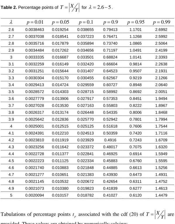
Table 2. Percentage points of T X Y = for λ =2.6 5− . λ p=0.01 p=0.05 p=0.1 p=0.9 p=0.95 p=0.99 2.6 0.0038463 0.019254 0.038655 0.79413 1.1701 2.6992 2.7 0.0037038 0.018541 0.037223 0.76471 1.1268 2.5992 2.8 0.0035716 0.017879 0.035894 0.73740 1.0865 2.5064 2.9 0.0034484 0.017262 0.034656 0.71197 1.0491 2.4199 3 0.0033335 0.016687 0.033501 0.68824 1.0141 2.3393 3.1 0.0032259 0.016149 0.032420 0.66604 0.9814 2.2638 3.2 0.0031251 0.015644 0.031407 0.64523 0.9507 2.1931 3.3 0.0030304 0.015170 0.030455 0.62567 0.9219 2.1266 3.4 0.0029413 0.014724 0.029559 0.60727 0.8948 2.0640 3.5 0.0028572 0.014303 0.028715 0.58992 0.8692 2.0051 3.6 0.0027779 0.013906 0.027917 0.57353 0.8451 1.9494 3.7 0.0027028 0.013530 0.027163 0.55803 0.8222 1.8967 3.8 0.0026317 0.013174 0.026448 0.54335 0.8006 1.8468 3.9 0.0025642 0.012836 0.025770 0.52942 0.7801 1.7994 4 0.0025001 0.012515 0.025125 0.51618 0.7606 1.7544 4.1 0.0024391 0.012210 0.024513 0.50359 0.7420 1.7116 4.2 0.0023810 0.011919 0.023929 0.4916 0.7243 1.6709 4.3 0.0023256 0.011642 0.023372 0.48017 0.7075 1.6320 4.4 0.0022728 0.011377 0.022841 0.46925 0.6914 1.5949 4.5 0.0022223 0.011125 0.022334 0.45883 0.6760 1.5595 4.6 0.0021740 0.010883 0.021848 0.44885 0.6613 1.5256 4.7 0.0021277 0.010651 0.021383 0.43930 0.6473 1.4931 4.8 0.0021145 0.010532 0.020672 0.42654 0.6311 1.4752 4.9 0.0021073 0.010380 0.019823 0.41839 0.6277 1.4613 5 0.0020094 0.010157 0.018782 0.41027 0.6120 1.4479

Tabulations of percentage points t_p associated with the cdf (20) of T X Y

= are

provided. These values are obtained by numerically solving:

p

t

p λ

Tables 1 and 2 provide the numerical values of t_p for λ=0.1, 0.2,..., 5 and σ =1. It is hoped that these numbers will be of use to practitioners as mentioned in the introduction. Similar tabulations could be easily derived for other values of ,λ σ and p by using the sample program provided in Appendix A.

References

Casella, G., & Berger, L. B. (2002), Statistical Inference. Duxbury Press. Gradshteyn, I. S., & Ryzhik, I. M. (2000).Table of Integrals, Series, and Products. San Diego, CA: Academic Press.

Greay R. C. (1930). The frequency distribution of the quotient of two normal variates. Journal of the Royal Statistical Society. 93, 442-446.

Helstrom, C. (1997). Computing the distribution of sums of random sine waves and the Rayleigh-distributed random variables by saddle-point integration.

IEEE Trans. Commun. 45(11), 1487-1494.

Karagiannidis, G. K., & Kotsopoulos, S. A. (2001). On the distribution of the weighted sum of L independent Rician and Nakagami Envelopes in the

presence of AWGN. Journal of Communication and Networks. 3(2), 112-119.

Marsaglia, G. (1965). Ratios of Normal Variables and Ratios of Sums of Uniform. JASA. 60, 193, 204.

Marsaglia, G. (2006). Ratios of Normal Variables. Journal of Statistical Software. 16(4), 1-10.

Nadarajah, S. (2006). Quotient of Laplace and Gumbel random variables.

Mathematical Problems in Engineering. vol. 2006. Article ID 90598, 7 pages. Pearson, K. (1910). On the constants of Index-Distributions as Deduced from the Like Constants for the Components of the Ratio with Special Reference to the Opsonic Index. Biometrika. 7(4), 531-541.

Prudnikov, A. P., Brychkov Y.A., Marichev O.I. (1986). Integrals and

Series, 2. New York:Gordon and Breach.

Rice, S. (1974). Probability distributions for noise plus several sin waves the problem of computation. IEEE Trans. Commun. 851-853.

Salo, J., EI-Sallabi, H. M., & Vainikainen, P. (2006). The distribution of the

product of independent Rayleigh random variables. IEEE Transactions on

Withers, C. S. & Nadarajah, S. (2008). MGFs for Rayleigh Random Variables. Wireless Personal Communications. 46(4), 463-468.

Appendix A

The following program in R can be used to generate tables similar to that presented in the section headed 'Percentiles.'

p=c(0.01,.05,0.1,0.9,0.95,0.99) sig=1 vlambda=seq(0.1,5,0.1) lvl=length(vlambda) mt=matrix(0,nc=length(p),nr=lvl) for(i in 1:lvl) { lambda=vlambda[i] t=p*sig*sqrt(1/(1-p^2))/lambda mt[i,]=t } print(mt)