Procedia Economics and Finance 30 ( 2015 ) 643 – 655
Available online at www.sciencedirect.com
2212-5671 © 2015 Published by Elsevier B.V. This is an open access article under the CC BY-NC-ND license (http://creativecommons.org/licenses/by-nc-nd/4.0/).
Peer-review under responsibility of IISES-International Institute for Social and Economics Sciences. doi: 10.1016/S2212-5671(15)01283-6
ScienceDirect
3rd Economics & Finance Conference, Rome, Italy, April 14-17, 2015 and 4th Economics &
Finance Conference, London, UK, August 25-28, 2015
Conditional Sovereign Transition Probability Matrices
Ahmet Perilioglu
a, Sukriye Tuysuz
b*
aIBM Algorithmics, Flat 11, 51 Commerell Street, London, SE100DZ, United Kingdom bYeditepe University, Kayisdagi Caddesi, Istanbul, 34755, Turkey
Abstract
Increase of credit derivative transaction volumes and credit related exposures in trading books, contingent effect of the recent financial crisis along with insufficient measure of so called Value At Risk calculations raised new methodologies for credit risk models as well as input parameters such as transition probability matrices. Conditional transition probability matrices are one of the main inputs of the credit risk models and it is required to estimate for short liquidity horizons. This study presents conditional transition probability matrices for sovereigns using factor modeling approaches under various symmetric and asymmetric distribution assumptions. Asymmetric models are found to provide superior results over the symmetric models for both in sample and out of sample results. Furthermore, the proposed methodology is applicable for quarterly sovereign transitions where rating movements are not observed frequently. Finally the model incorporates the dependence of the business cycles to the estimated credit cycle indices using main macroeconomic factors.
© 2015 The Authors. Published by Elsevier B.V.
Peer-review under responsibility of IISES-International Institute for Social and Economics Sciences.
Keywords: Transition probability; Credit rating; Credit risk; Sovereign debts; Business Cycles
1.Introduction
Transition probability matrix (TPM) plays a very crucial role in credit risk calculations. Recent credit risk models such as Incremental Risk Charge (IRC) require business cycle dependent, short term liquidity models (European Banking Authority, 2012). Tudela et al. (2012) showed that downgrades of ratings exceeded the upgrades of ratings during the subprime crises and an increase in rating volatility have been observed. Licari et al. (2013) studied stress
* Corresponding author. Tel.: +44-(0)-7760580631 , +90-(0)-2165783712
E-mail address: [email protected], [email protected]
© 2015 Published by Elsevier B.V. This is an open access article under the CC BY-NC-ND license (http://creativecommons.org/licenses/by-nc-nd/4.0/).
testing of credit migrations. Their study suggests that volatility of the rating transitions increase significantly and this leads to a bimodal rating distribution for trough the cycle models. In this case, imposing a symmetric distribution is not efficient and estimation will be biased.
Existing studies about the time-varying property of default rates and transition matrices can be separated into two groups. One group includes studies based on models for the valuation of derivative securities and credit related products in the risk neutral world (Jarrow et al., 1997; Lando, 1998; Hurd and Kuznetsov, 2006 and Andersson and Vanini, 2008). Jarrow et al. (1997) proposed a model for the term structure of credit spreads. Their model is based on the bankruptcy process with a discrete state space continuous time-homogeneous Markov chain in credit ratings which can be applied on observable market data. Lando (1998) generalized the model of Jarrow et al. (1997) and incorporated the dependence of term structure of interest rates on default intensities and transitions between rating categories.
Studies of the second group are concentrated on the modeling and estimation of default and migration probabilities. (Wilson, 1997; Belkin et al., 1998; Kim, 1999; Isreal et al., 2001; Hu et al., 2002; Wei, 2003; Truck, 2008 and Truck and Rachev, 2011). One of the first model for the conditioning of the transition probability matrix using macro-economic variables was presented by Wilson (1997). Belkin et al. (1998) initiated their studies on transition matrices in the form of single systematic credit factor. In the suggested one factor model credit factors follow a standard normal distribution. Kim (1999) applied a two-step procedure to condition transition probabilities using macroeconomic variables similar to Belkin et al. (1998). Truck (2008) used compared factor models with numerical adjusted methods. Wei (2003) extended the model to multi-factor model. According to this study, correlation between credit states in regular business cycles is weak and mostly correlated during recessionary and expansionary business cycles.
The purpose of the present study is to extend the existing factor models on corporate transition probability matrices to sovereigns applying different distribution assumptions. Rating transitions present non-normal distribution behavior and change dramatically during the stressed credit conditions (Licari et al., 2013). Contrary to the existing studies which use normal distribution, asymmetric behavior of the rating distributions are applied to improve the estimation power of conditional transition probability matrices. We also extend the existing standard normal assumption by incorporating a volatility term as a new parameter. Addition of credit cycle volatility captures rating variability for short time horizons.
The outline of this article is as follows. Section two summarizes a literature review on rating based migration matrices. Third section illustrates the methodology for credit cycle indices, associated factor models and conditional transition probability matrices. Fourth chapter presents empirical findings and last section concludes.
2.Literature Review
In a usual way, transition probability matrix is defined as:
ൌ ൦ ଵǡଵ ڮ ଵǡ ڮ ڮ ڮ ିଵǡଵ ڮ ିଵǡ Ͳ ڮ ͳ ൪ ( 1 )
where ǡ Ͳ for all i, j and σ ǡൌ ͳ
ୀଵ for all i. K = 8 and all the possible credit states are represented by AAA,
AA, A, BBB, BB, B, CCC, D according to Standard and Poor's rankings.
Transition probability matrices are built on credit state processes. Let ܵ ൌ ݏǡ ǥ ǡ ݏ be the credit states and let i,j = 1 ,2 ,...,K be the indices of all possible credit states with a decreasing order of credit quality. Credit state process can be defined as a Markov chain process over fixed time points ܵ௧ୀଵǡ ܵ௧ୀଶǡǥǡܵ௧ୀ. The process of credit states for
any time interval ߜݐ ൌ ݐଶെ ݐଵǡ ǥǡ ݐെ ݐିଵ can be represented on the transition probability matrix ܲఋ௧ൌ ǡሺߜݐሻ. For i and j we can define ሺߜݐሻ ൌ ሺݏሺݐሻȁݏሺݐିଵሻሻ is the probability of being in credit state j at time ݐ, conditional on being in credit state i at time ݐିଵ. Rating agencies estimate transition probabilities by using well known discrete time 'cohort' method. This method consists of estimating the transition probabilities such as:
ො୧ǡ୨ൌ ୧ǡ୨Τ୧ǡ ് , ( 2 )
where ܰ is the total number of firms in state i at the beginning of the estimation period and ܰǡ is the total number of transitions from state i to j during the estimation period.
Transition matrices can be transformed into a continuous form (e.g. generator matrix). The generator matrices present several advantages; the most viable is that it can be applied for any arbitrary horizon (Lando and Skodeberg, 2002). Although this presents manifold advantages, there is a chance of the nonexistence of a valid generator matrix to a given discrete-time transition. Given that, Jarrow et al. (1997) proposed some approximation methods to determine an adequate generator matrix. Israel et al (2001) proposed some conditions on the existence of true generator matrices.
In the literature, Markov assumption for the migration behavior was retained by Jarrow et al. (1997) and Israel et al (2001). By contrast, Frydman and Schuermann (2008) considered the hypothesis of non-markov migration behavior. Altman and Kao (1992), Bangia et al. (2002) rejected the first-order Markov property by testing rating drift or so-called path dependence. Some authors found that transition matrices are not homogeneous through time (Weber et al., 1998; Nickell et al., 2000; Bangia et al., 2002; Truck and Rachev, 2005). Most of these authors showed that default rates and credit spreads depend on the stage of the business cycles. Several other studies showed that transition probability matrices vary according to business cycles. (Carty and Fons, 1993; Wilson, 1997; Nickell et al., 2000; Bangia et al., 2002; Wei, 2003; Jafry and Schuermann, 2004; Truck, 2008).
3.Fitting Procedure for Transition Probability Matrices
Transition probability matrices can be represented as credit score matrices. This representation can be calculated with the inverse cumulative of a probability distribution function ܨሺǤ ሻିଵ on the average transition probability matrix (Gupton et al, 1997). This mapping methodology is expressed as:
ݖǡൌ ܨିଵ൫σୀଵҧǡǡ ߠ൯ǡ ( 3 )
where ҧǡ is the average transition probability and ߠ is a vector of parameters of the retained distribution.
For a given distribution, a credit score matrix can be constructed as:
ܼ ൌ
ݖଵǡଵ ڮ ݖଵǡ
ڮ ڮ ڮ
ݖିଵǡଵ ڮ ݖିଵǡ
൩ ( 4 )
The matrix can be illustrated as a sequence of joint bins as well. The last row of the transition probability matrix is for the absorbing state and it doesn’t change according to estimated time period, therefore it is omitted in the credit
score matrix.
For each period (every quarter in the present paper), deviations from the average credit scores is estimated. This deviation represents the credit cycles in relation with business cycles. According to Wei (2003) for a given credit state,
rating drift gives the directional change in all credit scores from its average value. While a positive rating drift means an increase in credit quality overall, a negative drift is a sign of deterioration in credit quality.
In most of the existing studies, the function ܨሺǤ ሻ is represented by the cumulative normal distribution function ሺߔሻ
(Wilson, 1997; Belkin et al., 1998; Kim, 1999; Wei, 2003; Lu and Kuo, 2006; Lu, 2007; Truck, 2008). This distribution is symmetric and thin-tailed. However, according to Licari et al (2013) rating transitions tend to have asymmetric distribution. These authors state that upgrade and downgrade momentum of the rating transition is not symmetric around the average value and they show different behaviors during the stress periods. Furthermore, their study points that volatility of the ratings varies across the quality of the rating classes, i.e. high quality ratings are more volatile than the low quality ratings. Similarly, Nickell et al. (2000) showed that decrease in credit quality leads to an increase in rating volatility. In this case, it is required to consider the volatility as well for different rating qualities.
Owing to the characteristics of rating transitions (fat-tailed and skewed), it would be more appropriate to build models on asymmetric distributions that represents the nature of the business cycles. For this reason, normal inverse Gaussian distribution is considered in this study. Factor models can be estimated without an adjustment of the distribution. Normal inverse Gaussian distribution holds the same property as the standard normal distribution, namely it is closed under convolution.
Using the calculated credit scores (matrix 3), the deviations from the average credit scores can be calculated as follows,
Ƹ௧ǡǡ ൌ ܨ൫ݖǡെ ݔ௧ǡǡ ߠ௧ǡ൯ െ σାଵǡାଵஸƸ௧ǡǡǡ ( 5 )
where ܨሺǤ ሻ is a cumulative distribution function. In this study it is either normal distribution or normal inverse Gaussian distribution. ݖǡ and ݔ௧ǡrepresent the credit scores from average matrix and the credit cycle index
(representing the deviations or rating drifts), respectively. As for Ƹ௧ǡǡ is the fitted transition probability for a given time period, And, c is an index of rating categories (i.e., IG for Investment Grade and NG for Non-Investment Grade) represented as a group of credit states and ߠ௧ǡ is the parameter vector.
The methodology to calculate the credit cycle indices is based on solving for the best fitting ݔ௧ǡand ߠ௧ǡ (unless it
is constant) such that the fitted transition probability matrix ܲ௧ǡ (defined in Eq.(5)) represents the observed transition probability matrix ܲ௧ǡ for a given time period t. In order to solve the credit cycle indices for each time period, an
optimization procedure to find the minimum of the distances between the actual and the fitted transition probability matrix is iteratively processed. In this paper, the sum of the squared error (SSE) is used to measure the distance error between the matrices due to good fitting results.
Existing studies (Belkin et al., 1998; Kim, 1999; Wei, 2003; Truck, 2008) on standard normal distribution set the parameter vector constant (mean=0 and standard deviation =1). In this paper the parameters vector is either constant or stochastic with a time index. Indeed, as emphasized by Nickell et al. (2000) and Licari et al. (2013), the changing nature of the volatility across different quality of ratings can be formalized by a stochastic behavior of rating volatility. For this reason in this study as a separate model, volatility parameter is considered to be stochastic under the normal distribution model and this is estimated within the vector of ߠ௧ǡ. On the other hand for the normal inverse Gaussian
distributions, to avoid further complexity and to compare the models under different asymmetric behaviors, ߠ௧is
arbitrarily selected to be constant. The density function of NIG distribution is characterized with the following parameters: ߤ(location), ߜ(scale), ߚ(asymmetry) and ߙ(tail heaviness). The parameters for the Normal Inverse Gaussian distribution are set toߙ ൌ ͳͲǡ ߤ ൌ Ͳǡ ߜ ൌ ͳ:. The skewness parameter for the Ⱦis selected to be positive/negative to allow a right/left skewness for the model. As ߚincrease the skewness of the density increase. In that sense, a high value ߚ ൌ ͻ is selected for right skewness (RS-NIG) and a low value ߚ ൌ െͻ is selected for left
skewness (LS-NIG). This is to ensure a very high degree of skewness along with a fast algorithm with a small Ƚ
parameter. In our study it is observed that upgrades/downgrades dynamics are more sensitive to higher positive/negative value of ߚ.
3.1.Factor Model Representations
In order to adjust transition probability matrices one factor and multi factor models were proposed. As presented by Belkin et al. (1998) one factor model is decomposed into systematic and idiosyncratic factors as,
ݕ௧ǡൌ ݓݔ௧ǡ ξͳ െ ݓଶߝ௧ǡǡ ( 6 )
where ୲ǡୡ represents the credit change indicator and ɂ୲ǡୡis the idiosyncratic factor or residual error. In the existing studies, variables ɂ୲ǡୡ and ୲ǡୡare assumed to be i.i.d. standard normal variables under the model structure, hence
applying the weighting guarantees that ୲ǡୡis also standard normal variable. Correlation structure between the credit
cycle index and credit change indicator is defined as ଶ.
Similarly, the multi-factor model of Wei (2003) is expressed as:
ݕ௧ǡൌ ݓ൫ݔ௧ ݔ௧ǡ൯ ξͳ െ ʹݓଶߝ
௧ǡǡ ( 7 )
where ݔ௧is the common factor and ୲ǡୡis the rating specific factor for each rating category c. Similar to the one
factor model, factors and idiosyncratic factor are assumed to be i.i.d. standard normal variables. In this equation the correlation between any two rating states are the same.
Frequently, unit diagonal entries in quarterly sovereign transition probability matrices are observed as opposed to corporate. Examples of the quarterly and annual transition probability matrices are available upon request. Estimation of w by using matrices with frequent unit diagonal entries and Eq.(6) or Eq.(7) usually provide undesirable results as calculation will be biased towards the unit entries. Therefore to handle this, it is possible to remove the adjustment factors on idiosyncratic term and model only the shifts in the credit cycle index. By considering these facts, we can formalize the dynamic of the credit change indicator with the a new factor model, which does not take into account the adjustment factor on idiosyncratic term in Eq.(6). The proposed factor model is then expressed as:
ݕ௧ǡൌ ݓݔ௧ǡ ߝ௧ǡ. ( 8 )
There are mainly two different estimation procedures for the w. While Belkin et al. (1998) proposed to use an ordered probit approach for the one factor model, Wei (2003) proposed to apply a one pass procedure to estimate the w and factor realizations for the multi factor model. Similar to the procedure applied on Eq.(5) in order to calculate the w and to adjust the transition probability matrix, a probit model is defined according to the rating drift dynamic on Eq.(8).
ሺݐǡ ݅ǡ ݆ȁݔ௧ǡǡ ߠ௧ǡሻ ൌ ܨ൫ݖǡെ ݓݔ௧ǡǡ ߠ௧ǡ൯ െ σ ൫ݐǡ ݅ǡ ݆หݔ௧ǡǡ ߠ௧ǡ൯ǡ
ାଵǡାଵஸ ( 9 )
where ݓ is the estimated value. ݔ௧ǡ and ߠ௧ǡare the previously estimated variables in equation Eq.(5).
The optimization procedure consists of minimizing the total distances (mean absolute error) between the observed transition probability matrices ܲ and the fitted transition matrices ܲȁ௫. In order to measure the distances, Truck 2008
applied two classical and two risk sensitive metrics. The classical distances, named total absolute error and sum of the squared error, are measured as:
ܦଵ൫ܲǡ ܲȁ௫൯ ൌ σିଵୀଵ σୀଵหሺݐǡ ݅ǡ ݆ሻ െ ൫ݐǡ ݅ǡ ݆หݔ௧ǡǡ ߠ௧ǡ൯หǡ ( 10 )
ܦଶ൫ܲǡ ܲȁ௫൯ ൌ ටσୀଵିଵσୀଵ ሺሺݐǡ ݅ǡ ݆ሻ െ ൫ݐǡ ݅ǡ ݆หݔ௧ǡǡ ߠ௧ǡ൯ሻଶǡ ( 11 )
The two risk sensitive distance measures are defined as:
ܦଵ൫ܲǡ ܲȁ௫൯ ൌ σିଵୀଵ σିଵୀଵ ݀ሺݐǡ ݅ǡ ݆ሻ σିଵୀଵ ܭǤ ݀ሺݐǡ ݅ǡ ܭሻǡ ( 12 )
ܦଶ൫ܲǡ ܲȁ௫൯ ൌ σିଵୀଵ σିଵୀଵ݀ሺݐǡ ݅ǡ ݆ሻ σିଵୀଵ ܭଶǤ ݀ሺݐǡ ݅ǡ ܭሻǡ ( 13 ) with ݀ሺݐǡ ݅ǡ ݆ሻ ൌ ሺ݅ െ ݆ሻሺሺݐǡ ݅ǡ ݆ሻ െ ሺݐǡ ݅ǡ ݆ȁݔ௧ǡǡ ߠ௧ǡሻሻ.
While the classical distance measures equally weight all the transition probabilities, the risk sensitive distance measures put more weight on far transitions according to initial rating grade.
The procedure estimates the w under different distance measures for each rating categories. The estimated w and credit cycle indices are then used to produce fitted transition probability matrices using the Eq.(9).
3.2.Rating Data and Credit Cycle Indices
In this paper cohort methodology is used to construct transition probability matrices. In order to capture within year rating movements, quarterly estimation horizon is selected. Rating data is obtained from regular publishing of Standard and Poor's Sovereign Rating and Country T and C Assessment Histories (2015), which contains credit rating history for 138 sovereign governments over the period from January 1975 to November 2014 with a total of 1799 rating assessment for long term foreign-currency rating category including not-rated (N.R.) state. As an industry standard, N.R. states are distributed on a pro rata basis (Jarrow et al., 1997; Jafry and Schuermann, 2004).
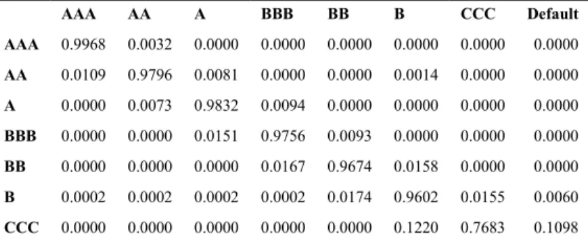
Credit cycles indices are estimated from transition probability matrices. In order to fully capture the migration effects, in sample period is selected from the beginning of 1996 to the end of 2010 in total of 60 quarters and out of sampling forecasting period is selected from the beginning of 2011 to the end of 2014 in total of 16 quarters. For this purpose, 76 quarterly transition probability matrices are estimated. Average transition probability matrix is estimated for in sample period and displayed in Table 1.
Table 1 - Average quarterly transition matrix for the period of 1996-2010
AAA AA A BBB BB B CCC Default AAA 0.9968 0.0032 0.0000 0.0000 0.0000 0.0000 0.0000 0.0000 AA 0.0109 0.9796 0.0081 0.0000 0.0000 0.0014 0.0000 0.0000 A 0.0000 0.0073 0.9832 0.0094 0.0000 0.0000 0.0000 0.0000 BBB 0.0000 0.0000 0.0151 0.9756 0.0093 0.0000 0.0000 0.0000 BB 0.0000 0.0000 0.0000 0.0167 0.9674 0.0158 0.0000 0.0000 B 0.0002 0.0002 0.0002 0.0002 0.0174 0.9602 0.0155 0.0060 CCC 0.0000 0.0000 0.0000 0.0000 0.0000 0.1220 0.7683 0.1098
In this paper, we construct four credit cycle models to fit the transition probability matrices to the observed transition probability matrices for in sample period. For each model, two credit cycle indices are estimated per rating categories i.e. investment grade (IG) and non-investment grade (NG). Models are displayed in Table 2.
Table 2 - Selected Models for Transition Probability Matrices
Model Model Name Distribution F(.) Estimates
X1 Standard Normal Standard Normal Drift
X2 Right Skewed NIG Normal Inverse Gaussian Drift
X3 Left Skewed NIG Normal Inverse Gaussian Drift
X4 Normal Extended Normal Drift and Volatility
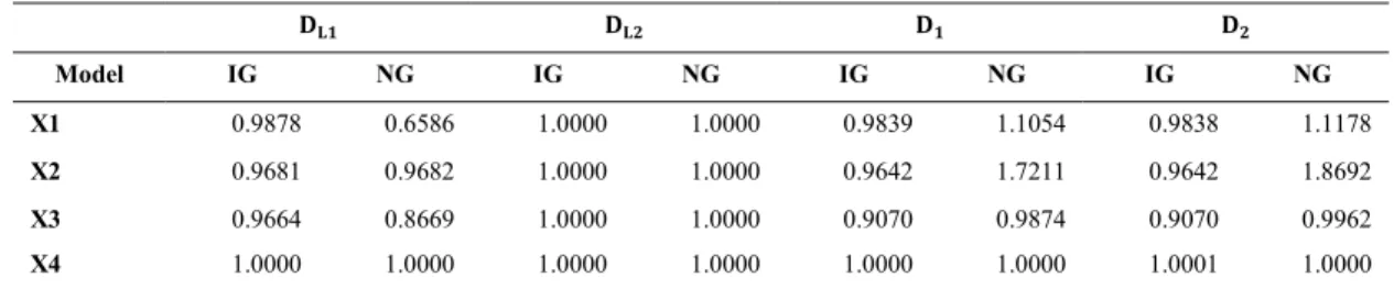
First, credit cycle indices are estimated for each model and each rating category (IG for investment grade and NG for non-investment grade) using equation Eq.(5). Once credit cycle indices are estimated, estimated values of w are determined using Eq.(9) for each model, rating category and distance measure to further adjust the transition matrices. Estimated w values are displayed in Table 3.
Table 3 – Estimated w for credit cycle indices
۲ۺ ۲ۺ ۲ ۲ Model IG NG IG NG IG NG IG NG X1 0.9878 0.6586 1.0000 1.0000 0.9839 1.1054 0.9838 1.1178 X2 0.9681 0.9682 1.0000 1.0000 0.9642 1.7211 0.9642 1.8692 X3 0.9664 0.8669 1.0000 1.0000 0.9070 0.9874 0.9070 0.9962 X4 1.0000 1.0000 1.0000 1.0000 1.0000 1.0000 1.0001 1.0000
Each pair of column represents estimated results using previously defined distance measures (e.g. Eq.(10), Eq.(11), Eq.(12) and Eq.(13). Most of the time estimates are close to 1 for both investment grade and non-investment grade categories. Results suggesting that estimated credit cycle indices well represent the systematic behavior of the rating transitions. Estimated values of w with the ܦଶ measure is equal to 1 and this is due to the fact that the same distance
measure is applied on the estimation of credit cycle indices. On the other hand unit estimates for normal extended model (X4) suggest a good fit with credit cycle indices and do not require a further fitting procedure to estimate the w.
In order to assess the performance of fitting for each fitted transition matrix, goodness of fit measures are calculated between the fitted and observed transition probability matrices. For this purpose, Wei 2003 proposes two measures: L-Factor statistic and Quasi R-square statistic. L-Factor statistic is calculated to measure the performance of absolute differences of fitted transition probability matrix against the observed transition probability matrix as:
ܮ െ ܨܽܿݐݎ௧ൌ ͳ െ ൬ σ಼షభసభ σ಼ೕసభȁǡǡೕషොǡǡೕȁ ିଵ ൰, ( 14 ) ܳݑܽݏ݅ െ ܴଶൌ ቆ ሺσసభσసభ಼షభσ಼ೕసభሺǡǡೕషҧǡǡೕሻሺොǡǡೕషҧǡǡೕሻሻ మ σసభσసభ಼షభσೕసభ಼ ൫ǡǡೕషҧǡǡೕ൯మσసభσ಼షభసభ σ಼ೕసభ൫ොǡǡೕషҧǡǡೕ൯మ ቇǤ ( 15 )
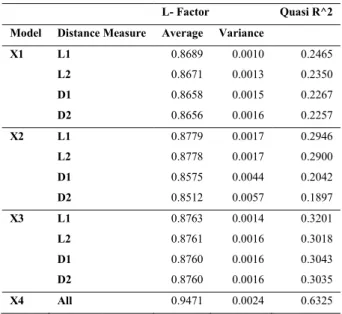
Table 4 - Goodness of fit measures for models
L- Factor Quasi R^2
Model Distance Measure Average Variance X1 L1 0.8689 0.0010 0.2465 L2 0.8671 0.0013 0.2350 D1 0.8658 0.0015 0.2267 D2 0.8656 0.0016 0.2257 X2 L1 0.8779 0.0017 0.2946 L2 0.8778 0.0017 0.2900 D1 0.8575 0.0044 0.2042 D2 0.8512 0.0057 0.1897 X3 L1 0.8763 0.0014 0.3201 L2 0.8761 0.0016 0.3018 D1 0.8760 0.0016 0.3043 D2 0.8760 0.0016 0.3035 X4 All 0.9471 0.0024 0.6325
Results in table 4 suggest that a significant improvement is achieved with models X2 and X3 compared to the standard model (X1). For instance according to classical distance measures (ଵand ଶ), there are approximately 20%
and 30% improvement in Quasi R-square for X2 and X3 respectively in comparison with X1. The good fitting results of asymmetric distributions support the findings of Licari et al. (2013). Precisely downgrade/upgrade oriented left/right skewed asymmetric distribution model illustrates a better fitting than the standard normal distribution model for all the distance measures. Volatility incorporated normal extended model (X4) improves the goodness of fit results approximately twofold and threefold in comparison with standard normal and asymmetric models respectively. However, in this model the number of latent variables doubles for estimation and prediction purposes.
Once the credit cycle indices are determined, a prediction model is built on the same using macroeconomic variables, credit spreads, market indices, early warning indicators or other credit indicators. The forecasted variables are then used to build a one factor or multi factor model to associate with the business cycle effects on conditional transition probability matrices.
3.3.Conditional Transition Probability Matrices
Advanced credit risk methodologies require the conditional transition probability matrices. Existing studies show that the prediction of the credit cycle index is performed by using macroeconomic variables. In this study, the retained macroeconomic variables are similar to the variables retained in most of the existing studies. These variables are the variation of GDP growth, the variation of the CPI, the variation of the unemployment rate and the spread between 10 year rate and 2 year rate. As this study is on global sovereigns, world macroeconomic variables are used. These quarterly macroeconomic variables cover the period between 1996 and 2014: the period from the beginning of 1996 until the end of 2010 constitutes the in sample period and the period from the beginning of 2011 until the end of 2014 the out of sample period.
Truck (2008) models the relation between the credit cycle index and macroeconomic variables with a multiple regression model. Autoregressive models have been also used in some of the existing studies. Wilson (1997) applied AR(2) to model the macroeconomic factors when conditioning the transition probability matrices and further
emphasized that a better model can be obtained using an ARMA(p,q) or a vector auto regressive moving average model. Similarly Licari et al. (2013) applied the vector autoregressive models on rating transitions to consider the dependency structure of the ratings with each other. In this article we model the relation between the credit cycle index (x) and macroeconomic variables (m) with a generalized autoregressive model with exogenous macroeconomic variables from lag 1 to lag 4 represented as,
୲ൌ Ⱦ σସ୧ୀଵɅ୧୲ି୧ σ୧ୀଵସ σ୨ୀଵସ Ⱦ୧ǡ୨୲ି୨ ɂ୲Ǥ ( 16 )
The macroeconomic variables ୲ି୨ are represented with the term݃݀௧ି,ܿ݅௧ି, ݑ݊݁݉௧ି, ݏݎ݁ܽ݀௧ି
respectively. Their impacts on the credit cycle index are measured with the ߚǡ parameters; where i and j represent the order of the lag and the macroeconomic variables, respectively. For instance, ߚଶǡଶ measures the impact of the
ܿ݅௧ିଶ.
Credit cycle index represents the rating activities throughout the business cycles. As in our study, Belkin (1998) and Wei (2003) applied the fitting procedure to calculate the credit cycle indices as a latent variable for each rating whereas Kim (1999) and Truck (2008) used the probability of default (pd) data as a credit cycle index. Our model is based on latent variables which represents the credit cycles of rating categories. Therefore, conditioning the transition probability matrices is constructed on models build on latent variables instead of probability of default as in previous studies. In this study we consider various models defined in Eq.(16) for standard normal and normal right/left inverse Gaussian models (X1, X2 and X3). Extended normal (X4) model requires additional modeling of volatility which has not been studied previously on factor models and we leave this as a further study. Once estimates/forecasts are calculated for credit cycle indices, Eq.(19) is recalculated to produce conditional transition probabilities.
4. Empirical Results
In this section, findings on various models and comparison of the conditional transition probability matrices are provided. For the estimation of Eq.(16), depending on the model, maximum likelihood method is employed using standard normal errors and normal inverse Gaussian errors. For out of sample prediction, coefficients are estimated in a recursive window. In general, credit risk calculations require one year ahead forecast and four quarter prediction is left for a further study.
The Eq.(16) is a generalized model comprising a total of 21 variables consist of 4 autoregressive, 4 macroeconomic variables with 4 lags and 1 constant. In order to avoid redundancy of the variables, 21 models are estimated for each credit cycle index by removing one of the least significant variables. Therefore the first model consists of all the variables and the last model contains only one variable. This allows a robust estimation and comparison methodology with most significant variables is preserved in the equations.
For prediction models, out of sample estimations are usually compared by using traditional metrics, such as root mean squared error (RMSE) and mean absolute error (MAE). Since the purpose of this article is to compare forecasted transition matrices, in this study (as previously by Truck, 2008) distance measures defined in Eq.(10), Eq.(11), Eq.(12) and Eq.(13) are used for out of sample model selection. Model with the lowest aggregated distance value is considered the most performing. For this aggregation, mean absolute error of distance measures between the conditional transition probability matrices and the observed transition probability matrices are calculated. Calculated distance measures of each model are available upon request. Selected models are grouped into per credit cycle index and per distance measures. Usually classic distance measures or risk sensitive distance measures per credit cycle index provides the same model. This indicates that there is not a significant difference between the selected models either on classic or risk sensitive measure. Contrary to the symmetric distribution models, asymmetric models provide significantly different models based on the selected distance measure.
Based on the out of sample results, once the retained models are obtained per credit cycle index and per risk sensitive measure, estimated equations are defined. Due to space, only details of the retained models for ܦଵ distance measure are presented in this paper. However results are available on request. In sample statistics of the retained models for each credit cycle index (X1, X2 and X3) according to ܦଵ distance measure are displayed in Table 5. Akaike and Bayesian Information Criteria (AIC and BIC) are presented for informative purposes.
Table 5 displays results of the best out of sample performing model. According to these results, the number of variables and the lags of those variables change across the models. Results show that third lag autocorrelation coefficient is significant for investment grade models. This supports the rating momentum when upgrades/downgrades are followed by previous upgrades/downgrades.
The significant values in the macro variables show that rating transitions vary according to the economic dynamics. Furthermore, results suggest that most of the time the sign of the variables are as expected. For instance GDP variations have a positive and significant impact in the X3 model. This result indicates that an increase of the GDP improves the credit quality. The impact of CPI is negative for IG and positive for NG. As expected, the negative impact indicates deterioration in the credit quality when CPI levels increase. However positive sign of the CPI indicates an improvement in the credit quality when the CPI levels increase. Usually low CPI is a sign of sustainable economy, however for non-investment grade category increase in price levels may be an indication of growing economy.
Table 5 - In sample and out of sample statistics of the retained models according to D(L1)
Coefficients Variables ͳ୍ୋ ͳୋ ʹ୍ୋ ʹୋ ͵୍ୋ ͵ୋ Ⱦ constant -0.2568 0.0821 (-1.7985) (0.6194) Ʌଵ ar(1) -0.0976 0.0628 (-0.7722) (0.6491) Ʌଶ ar(2) 0.1861 0.1386 -0.0691 (1.2373) (1.2112) (-0.5451) Ʌଷ ar(3) 0.3362 0.2958 (2.3416) (2.2976) Ʌସ ar(4) 0.2372 0.1631 0.1175 0.1157 (1.6092) (1.3238) (1.2305) (1.2546) Ⱦଵǡଵ ୲ିଵ 0.0775 -0.0802 0.1325 (1.4030) (-1.1282) (2.3605) Ⱦଵǡଶ ୲ିଶ 0.1003 0.0386 (1.9959) (0.6724) Ⱦଵǡଷ ୲ିଷ 0.0200 (0.3530) Ⱦଵǡସ ୲ିସ 0.0674 0.0682 0.0654 (1.3956) (1.2210) (1.1047) Ⱦଶǡଵ ୲ିଵ Ⱦଶǡଶ ୲ିଶ -0.1157 0.1826 -0.1243 0.2045 (-0.9790) (1.3888) (-0.8817) (1.8297)
Ⱦଶǡଷ ୲ିଷ -0.1806 0.3323 -0.2859 -0.1482 0.1767 (-1.5858) (2.4099) (-1.8165) (-1.2811) (1.3911) Ⱦଶǡସ ୲ିସ -0.2385 0.2057 -0.1448 (-1.8464) (1.4543) (-1.1870) Ⱦଷǡଵ ୲ିଵ -0.6151 -1.0590 0.3837 (-2.0985) (-2.6456) (1.0658) Ⱦଷǡଶ ୲ିଶ 0.8059 0.6863 (2.4532) (2.1249) Ⱦଷǡଷ ୲ିଷ Ⱦଷǡସ ୲ିସ Ⱦସǡଵ ୲ିଵ 0.3017 0.5109 0.1450 (1.9762) (2.3349) (0.6534) Ⱦସǡଶ ୲ିଶ -0.4026 (-1.1311) Ⱦସǡଷ ୲ିଷ -0.2823 -0.3548 0.1458 (-1.8106) (-1.9458) (0.6564) Ⱦସǡସ ୲ିସ ML -13.9301 -25.3713 -29.5619 -22.9717 -36.4404 -15.9127 AIC 45.8603 60.7427 85.1237 47.9433 78.8808 61.8254 BIC 64.7094 71.2144 112.3502 50.0377 85.1638 93.2405
* Values between (.) represent the t-statistics
Unemployment effect is mixed but tends to be statistically significant. Spread variable between 10 years and 2 years of the treasury rates illustrate flattening or steepening yield curve, of which steepening indicates a rising expectation on inflation or a higher economic growth. Sign of spread is usually positive for lower lags and negative for higher lags which indicate an increase in credit quality when the spread widens in short term and a decrease in credit quality in medium term.
Once the macroeconomic models are selected, conditional transition probability matrices can be compared according to distribution models. In sample and out of sample results are displayed in Table 6.
Table 6 - In sample and out of sample results of the conditional TPM models
Model In sample L1 L2 D1 D2 X1 0.9622 0.3889 1.2244 9.9491 X2 0.9763 0.3891 1.1998 9.0846 X3 0.9699 0.3835 1.1842 9.7342 Out of Sample
X1 1.1123 0.4781 2.3798 18.7834 X2 1.1339 0.4847 2.5858 19.1613 X3 1.0721 0.4681 2.3652 18.5467
In order to compare the models genuinely across each other, distance measures are presented in the table. Both in sample and out of sample results reveal that asymmetric distribution models (X2 and X3) outperform the standard normal models (X1) in general. X3 model illustrates a superior modeling for in sample and out of sample comparison, except from the first classic distance measure and last risk sensitive distance measure. Our findings confirm the requisite of the macroeconomic variables for modeling conditional transition probability matrices. We believe that a better estimation can be obtained by changing the lags of the autoregressive and macroeconomic variables.
4.Conclusions
In this paper conditional transition probability matrices are modeled under different distribution assumptions. It is observed that applying an asymmetric distribution such as a normal inverse Gaussian model instead of the standard normal model, improves the stability of the estimations significantly. The importance of transition probability matrices as a parameter to the credit risk models is important and it is desired to capture the adverse business conditions using a conditional model. There has been little attention to the modeling of the sovereign transition probability matrices in literature especially for less than a year of horizon. The methodology proposed in this paper improves the accuracy of the conditional sovereign transition probability matrices for short periods, therefore the loss figures for the credit models on short liquidity horizons such as IRC response better to the rapidly changing economic conditions.
References
Altman, E., and Kao, D., 1992. Rating drift of high yield bonds. Journal of Fixed Income 1(4), 15-20. Andersson, A., and Vanini, P., 2008. Credit migration risk modeling. Journal of Credit Risk.
European Banking Authority, 2012. EBA guidelines on the incremental default and migration risk charge.
Bangia, A., Diebold, F., Kronimus, A., Schagen, C., and Schuermann, T., 2002. Ratings migration and the business cycle with application to credit portfolio stress testing. Journal of Banking and Finance 26(2), 445-474.
Belkin, B., Suchower, S., Forest, L., and 1998. A one-parameter representation of credit risk and transition matrices, Creditmetrics Monitor 1(3), 46-56.
Carty, L., and Fons, J., 1994. Measuring changes in corporate credit quality. The Journal of Fixed Income 4(1), 27-41. Gupton, G., Finger, C., and Bhatia, M., 1997. Creditmetrics Technical Document, JP Morgan.
Hu, Y., Kiesel, R., and Perraudin, W., 2002. The estimation of transition matrices for sovereign credit ratings. Journal of Banking and Finance 26(7), 1383-1406.
Hurd, T., and Kuznetsov, A., 2007. Affine markov chain model of multifirm credit migration. Journal of Credit Risk 3(1), 3-29.
Israel, R., Rosenthal, J., and Wei, J., 2001. Finding generators for Markov chains via empirical transition matrices, with application to credit ratings. Mathematical Finance 11(2), 245-265.
Jafry, Y., and Schuermann, T., 2004. Measurement, estimation and comparison of credit migration matrices. Journal of Banking and Finance 28(11), 2603-2639.
Jarrow, R., Lando, D., and Turnbull, S., 1997. A Markov model for the term structure of credit risk spreads. The Review of Financial Studies 10(2), 481-523.
Kim, J., 1999. Conditioning the transition matrix. Risk, Credit Risk Special Report 37-40.
Lando, D., 1998. On Cox process and credit risky securities. Review of Derivatives Research 2(2-3), 99-120.
Lando, D., and Skodeberg, T., 2002. Analyzing ratings transitions and rating drift with continuous observations. Journal of Banking and Finance 26(2), 423-444.
Lu, S., and Kuo, C., 2006, The default probability of bank loans in Taiwan: An empirical investigation by Markov chain model. Asia Pacific Management Review 11(2), 111.
Lu, S., and Lee, K., 2007. An approach to condition the transition matrix on credit cycle: An empirical investigation of bank loans in Taiwan. Asia Pacific Management Review 12(2), 73.
Nickell, P., Perraudin, W., and Varotto, S., 2000. Stability of rating transitions. Journal of Banking and Finance 24(1), 203-227. Standard and Poors, 2015. Sovereign rating and country T. and C. assessment histories.
Truck, S., 2008. Forecasting credit migration matrices with business cycle effects-a model comparison. The European Journal of Finance 14(5), 359-379.
Truck, S., and Rachev, S., 2005. Credit portfolio risk and PD confidence sets through the business cycle. Working Paper SSRN 675622. Truck, S., and Rachev, S., 2011. Changes in migration matrices and credit VaR-A new class of difference indices. Working Paper SSRN 1787423. Wei, J., 2003. A multi-factor credit migration model for sovereign and corporate debts. Journal of International Money and Finance 22(5),
709-735.