Boston University
OpenBU
http://open.bu.edu
BU Open Access Articles BU Open Access Articles
2016-01-01
Mixed-criticality scheduling with I/O
This work was made openly accessible by BU Faculty. Please
share
how this access benefits you.
Your story matters.
Version
Accepted manuscript
Citation (published version): Eric Missimer, Katherine Missimer, Richard West. 2016.
"Mixed-Criticality Scheduling with I/O." Proceedings of the 28th
Euromicro Conference on RealTime Systems ECRTS 2016, pp. 120
-130 (11).
https://hdl.handle.net/2144/27915
Boston University
Mixed-Criticality Scheduling with I/O
Eric Missimer, Katherine Missimer and Richard West Computer Science Department
Boston University Boston, USA
Email:{missimer,kzhao,richwest}@cs.bu.edu
Abstract—This paper addresses the problem of scheduling tasks with different criticality levels in the presence of I/O requests. In mixed-criticality scheduling, higher criticality tasks are given precedence over those of lower criticality when it is impossible to guarantee the schedulability of all tasks. While mixed-criticality scheduling has gained attention in recent years, most approaches typically assume a periodic task model. This assumption does not always hold in practice, especially for real-time and embedded systems that perform I/O. In prior work, we developed a scheduling technique in the Quest real-time operating system, which integrates the time-budgeted management of I/O operations with Sporadic Server scheduling of tasks. This paper extends our previous scheduling approach with support for mixed-criticality tasks and I/O requests on the same processing core. Results show that in a real implementation the mixed-criticality scheduling method introduced in this paper outperforms a scheduling approach consisting of only Sporadic Servers.
Keywords-Mixed-criticality scheduling, I/O, real-time
I. INTRODUCTION
Mixed-criticality scheduling orders the execution of tasks of different criticality levels. Criticality levels are based on the consequences of a task violating its tim-ing requirements, or failtim-ing to function as specified. For example, DO-178B is a software certification used in avionics, which specifies several assurance levels in the face of software failures. These assurance levels range from catastrophic (e.g., could cause a plane crash) to non-critical when they have little or no impact on aircraft safety or overall operation. Mixed-criticality scheduling was first introduced by Vestal (2007) [1]. Later, Baruah, Burns and Davis (2011) [2] introduced Adaptive Mixed-Criticality (AMC) scheduling. The work presented in this paper builds upon AMC to extend it for use in systems where tasks make I/O requests. This is the first paper to address the issue of I/O scheduling in an Adaptive Mixed-Criticality scenario. Our approach to AMC with I/O is based on experience with our in-house real-time operating system, called Quest [3].
Quest has two privilege levels similar to UNIX-based systems, separating a trusted kernel space from a less privileged user space. In contrast, an alternative system configuration, called Quest-V, supports three privilege levels. The third privilege level in Quest-V is more trusted than the kernel, and operates as a lightweight virtual machine monitor, or hypervisor. Unlike with traditional virtual machine systems, Quest-V uses its most trusted privilege level to partition resources amongst (guest)
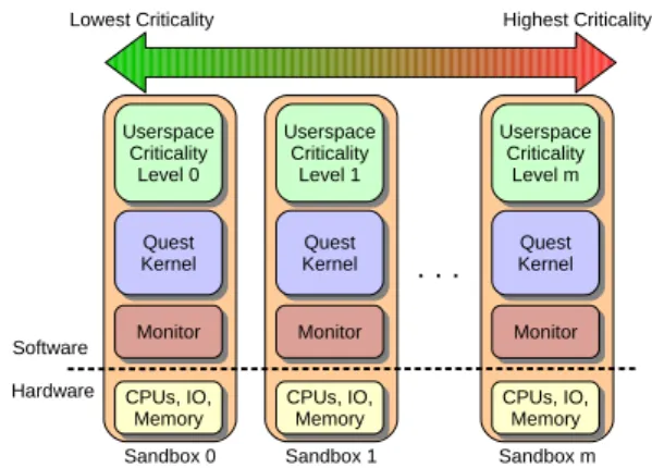
sandbox domains. Each sandbox domain then manages its own resources independently and in isolation of other sandbox domains, without recourse to a hypervisor. This leads to a far more efficient design, where virtualization overheads are almost entirely eliminated. It has been shown in prior work that it is possible to dedicate separate tasks of different criticality levels to different sandboxes in Quest-V [4]. This is demonstrated in Figure 1. Note that each sandbox has a different criticality level with level 0 being the least critical. However, Quest-V has thus far not considered tasks of different criticality levels within the same sandbox and, hence, for scheduling on the same (shared) processor cores.
In this paper, we show how to integrate task and I/O event scheduling in an Adaptive Mixed-Criticality [2] framework built within the Quest kernel. We extend Quest with support for mode changes between different criti-cality levels. This enables components of different levels to coexist in a single Quest-V sandbox or in a single Quest system, as depicted in Figure 2. A Quest-V system is therefore able to support more criticality levels than sandboxes, while a Quest system is able to differentiate between the importance of separate tasks.
Figure 1: Mixed-Criticality Levels Across Separate Quest-V Sandboxes
Previous mixed-criticality analysis assumes that all jobs in the system are scheduled under the same policy, typ-ically as periodic tasks. However, as previously shown by Danish, Li and West [5], using the same scheduling policy for both task threads and bottom half interrupt handlers1 results in lower I/O performance and larger
overheads. Specifically, the authors compared the Spo-radic Server (SS) [6] model for both main threads and bottom half interrupt handlers to using Sporadic Servers for main threads and Priority Inheritance Bandwidth-preserving Servers (PIBS) for bottom half threads. The results showed that by using PIBS for interrupt bottom half threads, the scheduling overheads are reduced and I/O performance is increased.
The contributions of this paper include a mixed-criticality analysis assuming threads are scheduled using either the Sporadic Server or PIBS scheduling model. It is shown that while a system of Sporadic Servers and PIBS has a slightly lower schedulability than a system of only Sporadic Servers from a theoretical point of view, in practice a real implementation of both scheduling policies results in Sporadic Server and PIBS outperforming a system of only Sporadic Servers.
The rest of the paper is organized as follows. Sec-tion II provides the necessary background informaSec-tion on Sporadic Servers and PIBS and introduces a response time analysis for them. Next, Section III briefly discusses the Adaptive Mixed-Criticality (AMC) model. Section IV contains the AMC scheduling analysis for a system of Sporadic and Priority Inheritance Bandwidth Preserving Servers. Section V discusses experimental results, while related work is described in Section VI. Finally, conclu-sions are discussed in Section VII.
II. SPORADICSERVER ANDPIBS
Sporadic Servers (SS) [6] and Priority Inheritance Bandwidth-preserving Servers (PIBS) [5] are the two scheduling models used in the Quest real-time operating system [3]. Sporadic Servers are specified using a budget capacity,C, and periodT. By default, the Sporadic Server with the smallest period is given highest priority, which follows the rate-monotonic policy [7]. The main tasks in Quest run on Sporadic Servers, thereby guaranteeing them a minimum share of CPU time every real-time period. Replenishment lists are used to track the consumption of CPU time and when it is eligible to be re-applied to the corresponding server.
PIBS uses a much simpler scheduling method which is more appropriate for the short execution times associated with interrupt bottom half threads. A PIBS is specified by a utilization, U. A PIBS always runs on behalf of a Sporadic Server and inherits both the priority and period of the Sporadic Server. For example, the PIBS running in response to a device interrupt would run on behalf of the Sporadic Server that requested the I/O action to
1We use the Linux terminology, where the top half is the
non-deferrable work that runs in interrupt context, and the bottom half is the deferrable work executed in a thread context after the top half.
be performed. The capacity of a PIBS is calculated as C=U×T, whereT is the period of the Sporadic Server.
As with a Sporadic Server, PIBS uses replenishments but instead of a list there is only asingle replenishment. When a PIBS has executedCactual, its next replenishment
is set tot+Cactual/U, wheretis the time the PIBS started
its most recent execution. A PIBS cannot execute again until the next replenishment time regardless of whether it has utilized its entire budget or not. Since a PIBS uses only one replenishment value rather than a list, it is beneficial for scheduling short-lived interrupt service routines that would otherwise fragment a Sporadic Server’s budget into many small replenishments. The replenishment method of a PIBS limits its maximum utilization within any sliding window of size T to (2−U)U. This occurs when the PIBS first runs for C1=U(T −U T) and then again for C2=U T. This is demonstrated in Figure 3:
C1+C2 T = (T′×U) +C 2 T = (T−C2)×U+C2 T = (C2/U−C2)×U+C2 C2/U = (2−U)U
Figure 3: PIBS Server Utilization
The interaction between Sporadic Servers and PIBS is depicted in Figure 4. First, the Sporadic Server initiates a blocking I/O related system call (Step 1). The system call invokes the associated device driver, which programs the device (Step 2). The device eventually raises an interrupt, which is handled by the top half handler (Step 3). The top half handler acknowledges the interrupt and wakes up one of the PIBS to handle the remaining bottom half work (Step 4). Finally, after a PIBS finishes executing it will wake up the corresponding Sporadic Server that was blocked on the I/O request (Step 5) [5].
If PIBS were replaced with a Sporadic Server, the short execution time of a bottom half interrupt handler may cause the server to block before exhausting its available capacity. This leads to a fragmented replenishment list. To reduce scheduling overheads and because of memory limits, Sporadic Server replenishment lists are kept to a finite length. When a replenishment list is full, items are merged to make space for new replenishments. This causes the available budget to be deferred [8], and the effective utilization of the Sporadic Server drops below its specified value. This in turn results in deadlines being missed. In contrast, a PIBS has only a single bandwidth preserving replenishment list item, leading to lower scheduling over-heads and increased effective utilization.
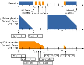
Figure 5 shows an example of replenishment list frag-mentation. A main task, τ1, wishes to execute for 8 time
units and then issues an I/O request (e.g., a blocking read) every period of 16 time units. A bottom half (BH) handler thread, τ2, associated with a Sporadic Server
(U = C T =
4
16), handles device interrupts corresponding
to I/O requests.τ1begins execution att=0and consumes
its entire budget before blocking on I/O. A single replen-ishment for 8 time units is posted at t=16, one period afterτ1started using its budget. Server replenishments are
shown in boxes as budget, time. Suppose an I/O event causes four interrupts to occur, each requiring a bottom half to execute for one time unit.τ1must wait for all four
interrupts to be handled before being able to resume. The first interrupt occurs at t=9 and is immediately handled by τ2. Also at t=9, the head replenishment list item for
the server associated withτ2is updated to a new starting
time. This is to ensure that a future replenishment is posted at the correct time. Once τ2 completes execution
of the bottom half interrupt handler, it blocks until another interrupt occurs.
When τ2 blocks it posts a replenishment item for
the capacity that it used. Since it used 1 time unit of capacity and started executing att=9, a replenishment of 1 time unit is posted at t=25. At t=11, another interrupt occurs, waking up τ2 for another time unit. The time
of the first replenishment list item is updated to 11 to reflect that the Sporadic Server started execution at that time. After handling the bottom half interrupt handler, another replenishment item for one time unit is posted, this time at t=27. When the third interrupt occurs, τ2
again executes for 1 time unit. However, whenτ2attempts
to post a subsequent replenishment, its server’s list is full.2 To ensure that τ2 does not adversely affect other
running tasks, its remaining capacity of one time unit is merged with the next replenishment list item, which in this example is att=25. This results in the available capacity forτ2 being zero, leaving it unable to immediately handle
the interrupt that occurs at t=15. Instead, the execution of the interrupt is delayed and completes only at t=26. Meanwhile,τ1, which had the capacity to execute att=16,
2For the sake of this example the replenishment list size is three.
In practice, a larger size would be chosen, but list fragmentation and capacity postponement are still possible [5].
is blocked waiting for completion of the fourth interrupt handler. τ1 begins execution at t=26, leaving only six
rather than eight time units until its deadline att=32.
Figure 5: Example Task and I/O Scheduling using Sporadic Servers
Figure 6 shows a similar scheduling scenario. However, this time the interrupt bottom halves are handled by a PIBS. As with the previous scenario, τ1 initiates an I/O
related event at t=8 and blocks until the completion of the event. The first interrupt occurs at t=9 and is immediately handled by PIBS. As with the Sporadic Server, the time in the replenishment list item is updated to reflect when the PIBS started execution. Once the event is handled, the PIBS posts a single replenishment item at t=13. This is because τ2 is running on behalf
of τ1, so it inherits both the priority and period of τ1.
Consequently, τ2 is eligible for execution again on its
server at te = t+Cactual/U = 9 + 1/0.25 = 13. The
second interrupt occurs att=11but its handling is deferred untilτ2has available capacity. Att=13, the third interrupt
arrives and τ2 has the capacity to handle both it and the
previous interrupt. Finally, the fourth interrupt arrives at t=15, which can also be handled by τ2. Since τ2 has
executed for 75% of its available capacity after processing the fourth interrupt, a replenishment is posted twelve time units after it started execution, att=25. This permitsτ1 to
continue execution att=16. The pattern then repeats itself. This simple example demonstrates the advantages of PIBS for bottom half threads compared to Sporadic Servers. Finally, note that even if the replenishment list in the first example had been long enough to avoid the delayed budget, the Sporadic Server would have experienced twice as much context switching overhead compared to the equivalent PIBS.
Note that in the first example, if a different policy for handling a full Sporadic Server replenishment list had been chosen, τ2 might have completed in time forτ1 to finish
before its deadline. For example, if the later replenishment items were merged instead of the head replenishment item, τ2would have had one remaining time unit of capacity to
Figure 6: Example Task and I/O Scheduling using Sporadic Servers & PIBS
more interrupts occur, this temporary fix will no longer work as more capacity is delayed further in time.
For systems where memory is plentiful, PIBS are ar-guably still preferential over Sporadic Servers for the man-agement of I/O events. Even if sufficient space exists for a highly fragmented replenishment list, a Sporadic Server may still experience a significant reduction in effective utilization. If the cost of reprogramming hardware timers is a non-trivial fraction of a budget replenishment, it makes sense to merge small replenishments into fewer larger ones. These merges lead to the same net effect as having finite replenishment lists, as described above.
A. Response Time Analysis for SS and PIBS
In order to perform an Adaptive Mixed-Criticality anal-ysis for a combined Sporadic Server and PIBS system, the response time analysis equation of the system must be derived. First, under the assumption that a Sporadic Server can be treated as an equivalent periodic task [6], the response time equation for taskτiin a system of only
Sporadic Servers is the following: Ri=Ci+ X τj∈hp(i) R i Tj Cj
wherehp(i)is the set of tasks of equal or higher priority than task τi. Second, due to the worst-case phasing of a
combined system of PIBS and Sporadic Servers, a PIBS utilization bound of (2−U)U cannot repeatedly occur. The worst case phasing can result in at most an additional capacity (i.e., execution time) of(Tq−TqUk)Uk for PIBS
τkassigned to the Sporadic Serverτq. This is only possible
if PIBS blocks waiting on I/O before consuming its full budget capacity. Therefore, a tighter upper-bound on the interference a PIBS can cause is:
Ikq(t) = (Tq−TqUk)Uk+ t Tq TqUk = (1−Uk)TqUk+ t Tq TqUk = 1 + t Tq −Uk TqUk
This can be incorporated into the response time analysis of Sporadic Serverτi, in a system consisting of both Sporadic
Servers and PIBS, in the following way: Ri=Ci+ X τj∈hp(i) Ri Tj Cj + X τk∈ps max τq∈hip(i) {Ikq(Ri)} (1)
Where ps is the set of all PIBS and hip(i) =hp(i)∪ {τi}, i.e. the set containing τi and all
tasks with equal or higher priority than task τi. This
is necessary as the PIBS can be running on behalf of task τi. In general, there is no a-priori knowledge about
which PIBS runs for which Sporadic Server. Therefore, the Sporadic Server, τq that maximizes the interference
caused by the PIBS must be considered. If such a-priori knowledge existed, it could be used to reduce the possible set of Sporadic Servers on behalf of which a PIBS could be executing. However, without such knowledge all possible Sporadic Server tasks of equal or higher priority must be considered.
The response time analysis for a PIBS is therefore dependent on the associated Sporadic Server. The response time analysis for PIBS τp when assigned to Sporadic
Serverτsis: sRp= (2−Up)UpTs+ X τj∈hip(s) sRp Tj Cj + X τk∈ps\{τp} max τq∈hip(s) {Ikq(sRp)} (2)
Note that (2−Up)UpTs is the maximum execution
time of the PIBS over a time window of Ts, i.e.
Is
p(Ts) = (2−Up)UpTs. Besides the first terms differing,
Equation 2 differs from Equation 1 in thathip(s)is used instead of hp(s)for the set of Sporadic Servers. This is because Sporadic Serverτsmust be included as it has an
equal priority to PIBSτpwhenτpis running on behalf of
τs. Also, the summation over all PIBS does not include
PIBSτp when determining its response time. IfsRp≤Ts,
for each and every Sporadic Server τs that τp can be
assigned to, thenτp will never miss a deadline.
III. BACKGROUND: AMC SCHEDULING
This section will provide the necessary background in-formation on Adaptive Mixed-Criticality (AMC) schedul-ing [2] to understand the analysis in Section IV. A more detailed analysis can be found in Baruah (2011) [2].
In AMC, a task τi is defined by its period, deadline,
a vector of computation times and a criticality level,
Ti, Di, ~Ci, Li
. In the simplest case, Li∈ {LO,HI}, i.e.
there are two criticality levels LO andHI where HI>LO. For tasks for whichL=LO,C(HI)is not defined as there are noHI-criticality versions of these tasks to execute. For HI-criticality tasksC(HI)≥C(LO). The system also has a criticality level and it initially starts in theLO-criticality mode. While running in theLO-criticality mode, bothLO
-andHI-criticality tasks execute, and while running inHI -criticality mode, only HI-criticality tasks execute. If a high-criticality task exhausts its C(LO) before finishing its current job, the system switches into theHI-criticality mode and suspends allLO-criticality tasks. This requires a signaling mechanism available to tasks to signal that they have completed execution of a specific job instance.
The schedulability test for AMC consists of three parts: 1) the schedulability of the tasks when the system is in the LO-criticality state, 2) the schedulability of the tasks when the system is in the HI-criticality state and 3) the schedulability of the tasks during the mode change from LO-criticality to HI-criticality. The first two are simple and can be handled with the traditional response time analysis, taking into account the appropriate set of tasks and worst case execution times. Specifically, the response time analysis for each task τi when the system is in the
LO-criticality state is: RLO i =Ci(LO) + X τj∈hp(i) RLO i Tj Cj(LO)
and the response time analysis for theHI-criticality state is: RHI i =Ci(HI) + X τj∈hpH(i) RHI i Tj Cj(HI)
where hpH(i)is the set of all high-criticality tasks with a priority higher than or equal to that of taskτi.
What remains is whether all HI-criticality tasks will meet their deadlines during the mode change from LO -criticality to HI-criticality. Baruah, Burns and Davis pro-vided two sufficient but not complete scheduling tests for the criticality mode, i.e. the tests will not admit task sets that are not schedulable but may reject task sets that are schedulable. The first is AMC-rtb (response time bound) which derives a new response time analysis equation for the mode change. The second is AMC-max which derives an expression for the maximum interference aHI -criticality task can experience during the mode change. AMC-max iterates over all possible points in time where the interference could increase, taking the maximum of these points. AMC-max is more computationally expen-sive than AMC-rtb but dominates AMC-rtb by permitting certain task sets that AMC-rtb rejects, and accepting any task set that AMC-rtb accepts. Both tests use Audsley’s priority-assignment algorithm [9], as priorities that are inversely related to period are not optimal for AMC [1], [2].
In this paper, we focus on the use of AMC-rtb for response time analysis of a system with Sporadic Servers and PIBS. This is because of the added expense incurred by AMC-max, which must iterate over all time points when LO-criticality tasks are released.
The AMC-rtb analysis starts with a modified form of the traditional periodic response time analysis:
R∗ i =Ci+ X τj∈hp(i) R∗ i Tj Cj(min (Li, Lj)) (3)
Where min (Li, Lj) returns the lowest criticality level
passed to it, e.g. in the case of a dual-criticality level system,HIis only returned if both arguments areHI. The use ofminimplies that we only consider criticality levels equal to or less than the criticality level ofτi. If we divide
the higher priority tasks by criticality level, we obtain the following: R∗i =Ci+ X τj∈hpH(i) R∗ i Tj Cj(min (Li, Lj)) + X τj∈hpL(i) R∗ i Tj Cj(LO) (4)
Where hpL(i) is the set of all LO-criticality tasks with a priority higher than or equal to the priority of task τi.
Theminin the third term is replaced withLOas we know Lj=LO. Since we are only concerned with high priority
tasks after the mode change, i.e. Li=HI, Equation 4
becomes: R∗i =Ci(HI) + X τj∈hpH(i) R∗ i Tj Cj(HI) + X τj∈hpL(i) R∗ i Tj Cj(LO) (5)
Finally, the response time bound can be tightened even further by recognizing that LO-criticality tasks can only interfere with HI-criticality tasks before the change has occurred. With this observation the final AMC response time bound equation is:
R∗i =Ci(HI) + X τj∈hpH(i) R∗ i Tj Cj(HI) + X τj∈hpL(i) RLO i Tj Cj(LO) (6)
A. LO-criticality tasks running in theHI-criticality mode Burns and Baruah [10] provide an extension to AMC that permits lower criticality tasks to continue execution in theHI-criticality state. This extension is used in our AMC model with support for I/O, which is briefly summarized as follows:
IfLO-criticality tasks are allowed to continue execution in theHI-criticality mode at a lower capacity, the following is the response time for a HI-criticality taskτi:
R∗i =Ci+ X τj∈hpH(i) R∗i Tj Cj(HI) + X τj∈hpL(i) RLO i Tj Cj(LO) + X τj∈hpL(i) R∗ i Tj − RLO i Tj Cj(HI) (7)
The final term in Equation 7 expresses the maximum number of times the LO-criticality task will be released multiplied by its smaller3 HI-criticality execution time.
3For LO-criticality tasks that can execute in HI-criticality mode,
While Equation 7 also applies toLO-criticality tasks that continue running after the mode change, a tighter bound is possible. Specifically, if aLO-criticality task has already run forC(HI)before the mode change then it has met its HI-criticality requirement. Therefore,RLOi can be replaced with a smaller value for LO-criticality tasks. To this end RLO∗
i is defined as the following:
RLO∗i = min (Ci(LO), Ci(HI)) + X τj∈hp(i) RLO∗ i Tj Cj(LO) (8)
Note thatRLO∗i =R LO
i if Li=HI andRLO∗i ≤R LO
i if Li=LO,
as LO-criticality tasks will have a smaller capacity in the HI-criticality mode. Therefore, Equation 7 can be replaced with the following more general equation that is tighter for LO-criticality tasks: R∗i =Ci+ X τj∈hpH(i) R∗ i Tj Cj(HI) + X τj∈hpL(i) RLO∗ i Tj Cj(LO) + X τj∈hpL(i) R∗ i Tj − RLO∗ i Tj Cj(HI) (9)
In Section IV we will use both AMC models described in this section to derive an AMC model for a system that includes Priority Inheritance Bandwidth-Preserving Servers.
IV. AMC SPORADICSERVER ANDPIBS SCHEDULING
This section describes the system model for I/O Adaptive Mixed-Criticality (IO-AMC), comprising both Sporadic Servers and Priority Inheritance Bandwidth-Preserving Servers (PIBS). IO-AMC focuses on the scheduling of I/O events and application threads in a mixed-criticality setting. Based on the IO-AMC model, we will derive a response time bound, IO-AMC-rtb, for Sporadic Servers and PIBS.
A. I/O Adaptive Mixed-Criticality Model
Sporadic Servers follow a similar model to the original AMC model. A Sporadic Server task τi is assigned a
criticality levelLi∈ {LO,HI}, a periodTi and a vector of
capacitiesC~i. The deadline is assumed to be equal to the
period. IfLi=LO,τi only runs while the system is in the
LO-criticality mode and therefore only C(LO) is defined. ForHI-criticality tasks bothC(LO)andC(HI)are defined andC(HI)≥C(LO).
For PIBS, an I/O task τk is again assigned to either
theLOorHIcriticality level;Lk∈ {LO,HI}. As previously discussed, PIBS are only defined by a utilizationUk. The
period, deadline and priority for a PIBS is inherited from the Sporadic Server for which it is performing a task. For IO-AMC, this definition is extended and each PIBS is defined by a vector of utilizations U~k. If τk is a LO
-criticality PIBS, i.e.Lk=LO, thenUk(LO)>Uk(HI)and if
Lk=HIthenUk(LO)≤Uk(HI). This definition allowsLO
-criticality PIBS to continue execution after the switch to HI-criticality. This model allows users to assign criticality levels to I/O devices indirectly by assigning criticality levels to the PIBS that execute in response to the I/O device.
With the typical AMC model now augmented to con-sider PIBS we can now derive a new admissions test for IO-AMC. First, the PIBS interference equation introduced in Section II is modified to incorporate criticality levels:
Ikq(t, L) = 1 + t Tq −Uk(L) TqUk(L)
As before, there are three conditions that must be considered: (1) the LO-criticality steady state, (2) the HI-criticality steady state, and (3) the change from LO -criticality toHI-criticality. The steady states are again sim-ple and are merely extensions of the non-mixed-criticality response time bounds. For Sporadic Server tasks the steady state equations are:
RLO i =Ci(LO) + X τj∈hp(i) RLO i Tj Cj(LO) + X τk∈ps max τq∈hip(i) Ikq RLO i ,LO (10) RHI i =Ci(HI) + X τj∈hpH(i) RHI i Tj Cj(HI) + X τk∈ps max τq∈hipH(i) Ikq R HI i ,HI (11)
where hipH(i) =hpH(i)∪ {τi}, i.e. it is the set of all
HI-criticality tasks of higher or equal priority than taskτi, plus taskτi itself. For PIBS taskτp, running on behalf of
Sporadic Server task τs, the steady state equations are:
sR LO p =(2−Up(LO))Up(LO)Ts + X τj∈hip(s) sRLOp Tj Cj(LO) + X τk∈ps\{τp} max τq∈hip(s) Ikq sR LO p ,LO (12) sR HI p =(2−Up(HI))Up(HI)Ts + X τj∈hipH(s) sRHIp Tj Cj(HI) + X τk∈ps\{τp} max τq∈hipH(s) Ikq sRHIp ,HI (13)
As with the traditional response time analysis of PIBS, its deadline is the same as that of its corresponding Sporadic Server τs. Therefore, the above analysis must be applied
to all Sporadic Servers associated with a PIBS. B. IO-AMC-rtb
The techniques described in Section III are used for the IO-AMC-rtb analysis. Specifically,LO-criticality PIBS are
allowed to continue execution in the HI-criticality mode. For a Sporadic Server task the IO-AMC-rtb equation is:
R∗i =Ci+ X τj∈hpH(i) R∗ i Tj Cj(HI) + X τj∈hpL(i) RLO∗ i Tj Cj(LO) + X τk∈psH max τq∈hip(i) Ikq(R ∗ i,HI) + X τk∈psL max τq∈hip(i) Ikq R LO∗ i ,LO + max τq′∈hipH(i) Ikq′ Ri∗−R LO∗ i ,HI (14) where psH andpsLare the set of HIandLO-criticality PIBS respectively. The last summation in Equation 14 represents the maximum interference aLO-criticality PIBS can cause. Specifically, Ikq(RLO
i ,LO) represents the
max-imum interference the PIBS can cause before the mode change and Ikq′(R∗i −R
LO
i ,HI) represents the total
inter-ference the PIBS can cause after the mode change. Again, the Sporadic Server that maximizes the interference is chosen for each PIBS.
The IO-AMC-rtb equation for a PIBSτkwhen assigned
to Sporadic Serverτsis:
sR∗p=(2−Up(HI))TsUp(HI) + X τj∈hipH(s) sR∗p Tj Cj(HI) + X τj∈hipL(s) sRLOp∗ Tj Cj(LO) + X τk∈(psH\{τp}) max τq∈hip(s) Ikq sR∗p,HI + X τk∈(psL\{τp}) max τq∈hip(s) Ikq sR LO∗ p ,LO + max τq′∈hipH(s) Ikq′ sR∗p−sR LO∗ p ,HI (15) Equation 15 differs from Equation 14 in the first term, and by the exclusion of τp from the set of PIBS. Similar to
Equation 2, the response time analysis requires iterating over all HI-criticality Sporadic Servers that could be associated with the PIBS. This is because only the HI -criticality Sporadic Servers are of interest after the mode change.
The work by Burns and Baruah [10] that allows LO -criticality periodic tasks to run in the HI-criticality mode can easily be applied to LO-criticality Sporadic Servers. This analysis is excluded for the sake of brevity.
V. EVALUATION
The experimental evaluation consists of two sections: 1) simulation-based schedulability tests, and 2) experiments conducted using the IO-AMC implementation in the Quest
operating system. The simulations show that a system of Sporadic Servers and PIBS has a similar but slightly lower schedulability than a system of only Sporadic Servers. This is due to the extra utilization requirement by PIBS compared to Sporadic Servers. However, the Quest exper-iments show the practical benefits of PIBS compared to Sporadic Servers, including how to control the criticality levels of I/O devices.
A. Simulation Experiments
In order to compare the proposed scheduling ap-proaches, random task sets were generated with varying total utilizations. 500 task sets were generated for each utilization value ranging from 0.20 to 0.95 with 0.05
increments. Each task set was tested to see if it was schedulable under the different policies. Each PIBS was randomly assigned to a single Sporadic Server of the same criticality level. For systems comprising only Sporadic Servers, the PIBS were converted to Sporadic Servers of equivalent utilization and period.4The parameters used to
generate the task sets are outlined in Table I.
Parameter Value
Number of Tasks 20 (15 Main, 5 I/O)
Criticality Factor 2
ProbabilityLi=HI 0.5
Period Range 1 – 100
I/O Total Utilization 0.05
Table I: Parameters Used to Generate Task Sets
The UUnifast algorithm [11] was used for task set generation, with task periods having a log-uniform distribution. For the mixed-criticality experi-ments, Ci(LO)=Ui/Ti. If Li=HI, Ci(HI)=CF×Ci(LO),
where CF is the criticality factor. For our experiments, if Li=LO,Ci(HI)=0.
The following are the different types of schedulability tests that were used in the evaluation. This includes schedulability tests for mixed-criticality and traditional systems.
• SS-rta– Sporadic Server response time analysis. Due to the nature of Sporadic Servers, this is the same as a periodic response time analysis.
• SS+PIBS-rta– Sporadic Server and PIBS response time analysis introduced in this paper. See Section II.
• AMC-rtb – Adaptive Mixed-Criticality response time bound developed by Baruah et al. [2]. See Section III.
• IO-AMC-rtb– I/O Adaptive Mixed-Criticality response
time bound developed in this paper. See Section IV.
• AMC UB– This is not a schedulability test but instead
an upper bound for AMC. It consists of both the LO -andHI-criticality level steady state tests. See Section III for details.
• IO-AMC UB – This is not a schedulability test but instead an upper bound for IO-AMC. It consists of both the LO- and HI-criticality level steady state tests. See Section IV for details.
1) SS+PIBS vs. SS-Only Simulations: Figure 7 shows the results of the response time analysis and event simula-tor for a system of Sporadic Servers and PIBS (SS+PIBS) compared to a system of only Sporadic Servers (SS-Only). As expected, a higher number of the Sporadic Server only task sets are schedulable using the response time analysis equations compared to the SS+PIBS response time analysis. This is due to the extra interference a PIBS can cause compared to a Sporadic Server of equivalent utilization and period.
0 % 20 % 40 % 60 % 80 % 100 % 0 0.2 0.4 0.6 0.8 1
Schedulable Task Sets
Utilization SS-rta
SS+PIBS-rta
Figure 7: Schedulability of SS+PIBS vs SS-Only
2) IO-AMC vs. AMC Simulations: In this section, IO-AMC is compared to an IO-AMC system containing only Sporadic Servers under different mixed-criticality scenar-ios.
Figure 8 shows the response time analysis and sim-ulation results when LO-criticality tasks do not run in the HI-criticality mode. Similar to Figure 7, AMC-rtb outperforms IO-AMC-rtb. This is due to the fact that AMC-rtb is an extension of the traditional response time analysis and does not experience the extra interference caused by PIBS. 0 % 20 % 40 % 60 % 80 % 100 % 0 0.2 0.4 0.6 0.8 1
Schedulable Task Sets
Utilization AMC UB
IO-AMC UB AMC-rtb IO-AMC-rtb
Figure 8: Schedulability of IO-AMC vs AMC
We also varied task set parameters to identify their effects on schedulability. For each set of parameterspin a given test y, we measured the weighted schedulabil-ity [12], which is defined as follows:
Wy(p) = X ∀τ (u(τ)×Sy(τ, p))/ X ∀τ u(τ)
where Sy(τ, p) is the binary result (0 or 1) of the
schedulability test y on task set τ, and u(τ) is the total utilization. The weighted schedulability compresses
a three-dimensional plot to two dimensions and places higher value on task sets with higher utilization.
Figures 9, 10, and 11 show the results of varying the probability of a HI-criticality task, the criticality factor, and the number of tasks, respectively. In all scenarios, LO-criticality tasks do not run in the HI-criticality mode. As expected, the percentage of schedulable tasks for IO-AMC is slightly lower than the percentage for traditional AMC. This is again due to the slightly larger interference caused by a PIBS. 0 % 20 % 40 % 60 % 80 % 100 % 0 0.2 0.4 0.6 0.8 1 Weighted Schedulability
Percentage of Tasks with High Criticality AMC UB
IO-AMC UB AMC-rtb IO-AMC-rtb
Figure 9: Weighted Schedulability vs % ofHI-criticality Tasks
0 % 20 % 40 % 60 % 80 % 100 % 1 1.5 2 2.5 3 3.5 4 4.5 5 Weighted Schedulability Criticality Factor AMC UB IO-AMC UB AMC-rtb IO-AMC-rtb
Figure 10: Weighted Schedulability vs Criticality Factor
0 % 20 % 40 % 60 % 80 % 100 % 0 20 40 60 80 100 Weighted Schedulability Number of tasks AMC UB IO-AMC UB AMC-rtb IO-AMC-rtb
Figure 11: Weighted Schedulability vs Number of Tasks
B. Quest Experiments
The above simulation results do not capture the practical costs of a system of servers for tasks and interrupt bottom halves. This section investigates the performance of our IO-AMC policy in the Quest real-time system. We also
study the effects of mode changes on I/O throughput for an application that collects streaming camera data. All experiments were run on a 3.10 GHz IntelR Core i3-2100
CPU.
1) Scheduling Overhead: We studied the scheduling overheads for two different system implementations in Quest. In the first system, Sporadic Servers were used for both tasks and bottom halves (SS-Only). In the second system, Sporadic Servers were used for tasks, and PIBS were used to handle interrupt bottom halves (SS+PIBS). In both cases, a task set consisted of two application threads of different criticality levels assigned to two dif-ferent Sporadic Servers, and one bottom half handler for interrupts from a USB camera. The first application thread read all the data available from the camera in a non-blocking manner and then busy-waited for its entire budget to simulate the time to process the data. The second appli-cation thread simply busy-waited for its entire budget, to simulate a CPU-bound task without any I/O requests. Both application threads consisted of a sequence of jobs. Each job was released once every server period or immediately after the completion of the previous job, depending on which was later. The experimental parameters are shown in Table II. Task C(LO)orU(LO) C(HI)orU(HI) T Application 1 (HI-criticality) 23ms 40ms 100ms Application 2 (LO-criticality) 10ms 1ms 100ms Bottom Half (PIBS) U(LO) = 1% U(HI) = 2% 100ms Bottom Half (SS) 1ms 2ms 100ms
Table II: Quest Task Set Parameters for Scheduling Overhead
The processor’s timestamp counter was recorded when each application finished its current job. Results are shown in Figure 12. For SS+PIBS, each application completed its jobs at regular intervals. However, for SS-Only, the HI-criticality server for interrupts from the USB camera caused interference with the application tasks. This led to theHI-criticality task depleting its budget before finishing its job. This is due to the extra overhead added by a Sporadic Server handling the interrupt bottom half thread. Therefore, the system had to switch into theHI-criticality mode to ensure the HI-criticality task completed its job, sacrificing the performance of theLO-criticality task. This is depicted by the larger time between completed jobs in Figure 12. The SS+PIBS task set did not suffer from this problem due to the lower scheduling overhead caused by PIBS.
Figure 13 shows the additional overhead caused when Sporadic Servers are used for bottom half threads as opposed to PIBS. This higher scheduling overhead is the cause for the mode change in the previous experiment. Figure 13 depicts two different system configurations, one involving only a single camera and another involving two cameras. For each configuration, the scheduling overhead for both SS-Only and SS+PIBS was measured. For the
0 1 2 3 4 5
Server Type
Time (seconds)
HI-Criticalty Task (SS+PIBS) LO-Criticalty Task (SS+PIBS) HI-Criticalty (SS-Only) LO-Criticalty (SS-Only)
Figure 12: Job Completion Times for SS+PIBS vs SS-Only
single camera configuration, there is one HI-criticality task, one LO-criticality task, and one HI-criticality server (either PIBS or Sporadic Server) for the USB camera interrupt bottom half thread. The scheduling overhead for SS-Only is more erratic and higher than the system of Sporadic Servers and PIBS. The second configuration adds a LO-criticality camera with a 2% utilization in the LO-criticality mode, a 1% utilization in theHI-criticality mode, and a period of 100 microseconds when utilizing a Sporadic Server. Figure 13 shows that the scheduling overhead for an SS-Only system more than doubled, going from an average of 0.21% to 0.49%, while an SS+PIBS system experienced only a small increase of0.03%.
0 0.1 0.2 0.3 0.4 0.5 0.6 0.7 0.8 0 20 40 60 80 100 120 140 160 180 CPU % Time (seconds) SS-Only (2 Camera) SS-Only (1 Camera) SS+PIBS (2 Camera) SS+PIBS (1 Camera)
Figure 13: Scheduling Overheads for SS-Only vs SS+PIBS
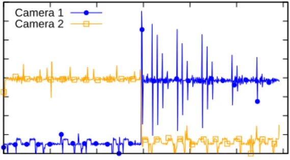
2) Mode Change for I/O Device: As mentioned in Section IV, assigning criticality levels to bottom half interrupt handlers is akin to assigning criticality levels to the device associated with the bottom half. To test this assertion, two USB cameras were assigned different criticality levels and a mode change was caused during the execution of the task set. The task set consisted of two Sporadic Servers and two PIBS, as shown in Table III.
Figure 14 shows the camera data available at each data point. At approximately 30 seconds, a mode change occurs that causes Camera 1 to change from a utilization of 0.1% to 1%, thereby increasing the amount of data received. Also at the time of the mode change, Camera 2’s utilization switches from 1% to0.1%, causing a drop in received data. The variance for Camera 1 after the mode
Task C(LO)orU(LO) C(HI)orU(HI) T Application 1 (HI-criticality) 25ms 40ms 100ms Application 2 (LO-criticality) 25ms 24ms 100ms Camera 1 - PIBS (HI-criticality) U(LO) = 0.1% U(HI) = 1% 100ms Camera 2 - PIBS (LO-criticality) U(LO) = 1% U(HI) = 0.1% 100ms
Table III: Quest Task Set Parameters for I/O Device Mode Change
change is due to extra processing of the delayed data that is performed by the bottom half interrupt handler. Finally, Figure 15 shows the total data processed from each camera over time. 0 5000 10000 15000 20000 25000 30000 35000 40000 0 10 20 30 40 50 60 Bytes Read Time (seconds) Camera 1 Camera 2
Figure 14: Data FromHI- andLO-criticality USB Cameras
0 1e+06 2e+06 3e+06 4e+06 5e+06 6e+06 7e+06 0 10 20 30 40 50 60
Total Bytes Read
Time (seconds) Camera 1
Camera 2
Figure 15: Total Data Processed Over Time
VI. RELATEDWORK
This section discusses related work in the areas of mixed-criticality and I/O-aware scheduling, beyond that already covered in Sections II and III.
In recent years, there have been many extensions to the Adaptive Mixed-Criticality model. For single core scheduling, Barauh, Burns and Davis extended their orig-inal AMC model to allow priorities to change [13]. Burns and Davis also introduced AMC-NPR (Non-Preemptive Region), which improved schedulability by permitting tasks to have a final non-preemptive region at the end of a job [14]. Fleming and Burns extended the AMC model to allow more than two criticality levels [15]. These variations on the mixed-critical model could be incorporated into the IO-AMC model.
Li and Barauh [16] combined the EDF-VD [17] single-core mixed-criticality approach with fpEDF [18], to de-velop a multi-core mixed-criticality scheduling algorithm. Pathan also developed a multi-core fixed priority schedul-ing algorithm for mixed-criticality [19]. This was an adaptation of the original single-core AMC approach to a multi-core scheduling framework compatible with Audsley’s algorithm [9]. The work by Pathan is more easily incorporated into the IO-AMC model given that both approaches use fixed priorities.
Lewandowski et al. [20] investigated the use of sporadic servers to appropriately budget bottom half threads, as part of an Ethernet NIC device driver. Zhang and West developed a process-aware interrupt scheduling and ac-countability scheme in Linux, to integrate the management of tasks and I/O events [21]. A similar approach was also implemented in the LITMUS kernel for GPGPUs on multiprocessor systems [22].
VII. CONCLUSIONS
This paper builds on our scheduling framework in the Quest real-time operating system, comprising a collec-tion of Sporadic Servers for tasks and Priority Inheri-tance Bandwidth-Preserving Servers (PIBS) for interrupt handlers. We first show a response time analysis for a collection of Sporadic Servers and PIBS in a system with-out mixed-criticality levels. We then extend the analysis to support an I/O Adaptive Mixed-Criticality (IO-AMC) model in a system comprising of tasks and interrupt han-dlers. Our IO-AMC response time bound considers a mode change to high-criticality when insufficient resources exist for either high-criticality tasks or interrupt handlers in low-criticality mode. The analysis considers the interference from low-criticality tasks and interrupt handlers before the mode change.
Simulation results show that a system of only Sporadic Servers for both tasks and interrupt handlers has a higher theoretical number of schedulable task sets. However, in practice, using PIBS to handle interrupts is shown to be superior because of lower system overheads. This paper also shows experimental results in the Quest real-time operating system, where criticality levels are assigned to devices. This enables high-criticality devices to gain more computational time when insufficient resources exist to service both high- and low-criticality tasks and interrupt bottom halves. In turn, this enables high-criticality tasks that issue I/O requests to be granted more CPU time to meet their deadlines.
The analysis in this paper assumes that tasks and I/O bottom half interrupt handlers are executed on separate servers that are independent of one another. In practice, a task may be blocked from execution until a pending I/O request is completed. As long as the I/O request is handled within the time that a task is waiting for its server to have its budget replenished, and is therefore ineligible to run, then our analysis holds. Future work will consider more complex task models where I/O requests can lead to blocking delays that impact the execution of tasks.
ACKNOWLEDGMENT
This material is based upon work supported by the National Science Foundation under Grant # 1117025 and 1527050. Any opinions, findings, and conclusions or rec-ommendations expressed in this material are those of the author(s) and do not necessarily reflect the views of the National Science Foundation.
REFERENCES
[1] S. Vestal, “Preemptive Scheduling of Multi-criticality Sys-tems with Varying Degrees of Execution Time Assurance,” inProceedings of the 28th IEEE Real-Time Systems Sym-posium, 2007, pp. 239–243.
[2] S. K. Baruah, A. Burns, and R. I. Davis, “Response-time Analysis for Mixed Criticality Systems,” inProceedings of the 32nd IEEE Real-Time Systems Symposium, 2011. [3] “Quest,” http://www.QuestOS.org.
[4] Y. Li, R. West, and E. Missimer, “A Virtualized Separation Kernel for Mixed Criticality Systems,” inProceedings of the 10th ACM SIGPLAN/SIGOPS International Conference on Virtual Execution Environments, 2014, pp. 201–212. [5] M. Danish, Y. Li, and R. West, “Virtual-CPU Scheduling
in the Quest Operating System,” inProceedings of the 17th IEEE Real-Time and Embedded Technology and Applica-tions Symposium, 2011, pp. 169–179.
[6] B. Sprunt, “Aperiodic Task Scheduling for Real-time Sys-tems,” Ph.D. dissertation, Carnegie Mellon University, 1990.
[7] C. L. Liu and J. W. Layland, “Scheduling Algorithms for Multiprogramming in a Hard Real-time Environment,”
Journal of the ACM, vol. 20, no. 1, pp. 46–61, 1973. [8] M. Stanovich, T. P. Baker, A. Wang, and M. G. Harbour,
“Defects of the POSIX Sporadic Server and How to Correct Them,” in Proceedings of the 16th IEEE Real-Time and Embedded Technology and Applications Symposium, 2010, pp. 35–45.
[9] N. C. Audsley, “On Priority Assignment in Fixed Priority Scheduling,”Information Processing Letters, vol. 79, no. 1, pp. 39–44, 2001.
[10] A. Burns and S. Baruah, “Towards a More Practical Model for Mixed Criticality Systems,” in The 1st Workshop on Mixed-Criticality Systems (colocated with RTSS), 2013.
[11] E. Bini and G. C. Buttazzo, “Measuring the Performance of Schedulability Tests,” Journal of Real-Time Systems, vol. 30, no. 1–2, pp. 129–154, 2005.
[12] A. Bastoni, B. Brandenburg, and J. Anderson, “Cache-related Preemption and Migration Delays: Empirical Ap-proximation and Impact on Schedulability,”OSPERT, pp. 33–44, 2010.
[13] S. Baruah, A. Burns, and R. Davis, “An Extended Fixed Priority Scheme for Mixed Criticality Systems,” Proc. ReTiMiCS, RTCSA, pp. 18–24, 2013.
[14] A. Burns and R. Davis, “Adaptive Mixed Criticality Scheduling with Deferred Preemption,” in Proceedings of the 35th IEEE Real-Time Systems Symposium, 2014. [15] T. Fleming and A. Burns, “Extending Mixed Criticality
Scheduling,” in The 1st Workshop on Mixed-Criticality Systems (colocated with RTSS), 2013.
[16] H. Li and S. Baruah, “Global Mixed-Criticality Scheduling on Multiprocessors,” inProceedings of the 24th Euromicro Conference on Real-Time Systems, vol. 12, 2012. [17] S. K. Baruah, V. Bonifaci, G. D’Angelo, A.
Marchetti-Spaccamela, S. Van Der Ster, and L. Stougie, “Mixed-Criticality Scheduling of Sporadic Task Systems,” in Pro-ceedings of the 19th Annual European Symposium on Algorithms. Springer, 2011, pp. 555–566.
[18] S. K. Baruah, “Optimal Utilization Bounds for the Fixed-priority Scheduling of Periodic Task Systems on Identi-cal Multiprocessors,” IEEE Transactions on Computers, vol. 53, no. 6, pp. 781–784, 2004.
[19] R. M. Pathan, “Schedulability Analysis of Mixed-criticality Systems on Multiprocessors,” in Proceedings of the 24th Euromicro Conference on Real-Time Systems, 2012, pp. 309–320.
[20] M. Lewandowski, M. J. Stanovich, T. P. Baker, K. Gopalan, and A. Wang, “Modeling Device Driver Effects in Real-time Schedulability Analysis: Study of a Network Driver,” inProceedings of the 13th IEEE Real Time and Embedded Technology and Applications Symposium, 2007, pp. 57–68. [21] Y. Zhang and R. West, “Process-aware Interrupt Scheduling and Accounting,” in Proceedings of the 27th IEEE Real-Time Systems Symposium, 2006, pp. 191–201.
[22] G. A. Elliott and J. H. Anderson, “Robust Real-time Multiprocessor Interrupt Handling Motivated by GPUs,” in
Proceedings of the 24th Euromicro Conference on Real-Time Systems, 2012, pp. 267–276.