Multiple testing problems in classical clinical trial and adaptive designs

OpenBU http://open.bu.edu

Theses & Dissertations Boston University Theses & Dissertations

2018

Multiple testing problems in

classical clinical trial and adaptive

designs

https://hdl.handle.net/2144/33080 Boston University

GRADUATE SCHOOL OF ARTS AND SCIENCES

Dissertation

MULTIPLE TESTING PROBLEMS IN CLASSICAL

CLINICAL TRIAL AND ADAPTIVE DESIGNS

by

XUAN DENG

B.S., University of Science and Technology Beijing, 2011

M.S., Brown University, 2013

Submitted in partial fulfillment of the

requirements for the degree of

Doctor of Philosophy

2018

First Reader

Mark Chang, Ph.D.

Adjunct Professor of Biostatistics

Second Reader

Gheorghe Doros, Ph.D. Professor of Biostatistics

Third Reader

Sandeep Menon, Ph.D.

A number of people have supported and helped me for the past five years to whom I am grateful from the bottom of my heart. This dissertation would not be complete without giving thanks to those people.

First, and foremost, I would like to send my sincere thanks to my thesis advisor, Dr. Mark Chang, for his guidance and encouragement throughout my long academic journey towards this degree. Dr. Chang is a motivated and inspired mentor, who always provided the constant support and advice as I worked on the dissertation. I valued his constructive opinions and appreciated his help to find the path forward during the whole process.

I would like to thank Dr. Gheorghe Doros and Dr. Sandeep Menon for being my dissertation readers. Their criticism and unique perspective during each thesis committee meeting always provided me another way to consider the problems. I also appreciate Dr. Michael Lavalley and Dr. Joe Massoro for agreeing to serve on my committee and am grateful for their time and suggestions.

I would like to thank Dr. L. Adrienne Cupples for being my academic advisor. She helped me to get used to the life and research study in the beginning of my program track. Her patience, enthusiasm and rigor have taught me how to be a qualified researcher. It has been a great delight to work with her. I would also like to thank Dr. Ching-Ti Liu for the opportunity he provided me to work with him during my time in the program. His valuable insight and discussion and generous resources in

I would not be here without the unconditional support and love from my family, I am so grateful for their understanding and encouragement when I questioned myself during the study. Last, but not the least, I would like to thank my research mates and friends: Virginia Fisher, Elise Lim, and Hanfei Xu for the study experience that we shared during this period.

CLINICAL TRIAL AND ADAPTIVE DESIGNS

XUAN DENG

Boston University, Graduate School of Arts and Sciences, 2018

Major Professor: Mark Chang, Adjunct Professor of Biostatistics

ABSTRACT

Multiplicity issues arise prevalently in a variety of situations in clinical trials and statistical methods for multiple testing have gradually gained importance with the increasing number of complex clinical trial designs. In general, two types of multiple testing can be performed (Dmitrienko et al., 2009): union-intersection testing (UIT) and intersection-union testing (IUT). The UIT is of the interest in this dissertation. Thus, the familywise error rate (FWER) is required to be controlled in the strong sense.

A number of methods have been developed for controlling the FWER, including single-step and stepwise procedures. In single-step approaches, such as the simple Bonferroni method, the rejection decision of a hypothesis does not depend on the decision of any other hypotheses. Single-step approaches can be improved in terms of power through stepwise approaches, while also controlling for the desired error rate.

the first project, we developed a new and powerful single-step progressive parametric multiple (SPPM) testing procedure for correlated normal test statistics. Through simulation studies, we demonstrate that SPPM improves power substantially when the correlation is moderate and/or the magnitude of effect sizes are similar.

Group sequential designs (GSD) are clinical trials allowing interim looks with the possibility of early terminations due to efficacy, harm or futility, which can reduce the overall costs and timelines for the development of a new drug. However, repeated looks of data also have multiplicity issues and could inflate the type I error rate. The proper treatments to the error inflation have been discussed widely (Pocock, 1977), (O’Brien and Fleming, 1979), (Wang and Tsiatis, 1987), (Lan and DeMets, 1983). Most literature about GSD focuses on a single endpoint. GSD with multiple endpoints however, has also received considerable attention. The main focus of our second project is a GSD with multiple primary endpoints, in which the trial is to evaluate whether at least one of the endpoints is statistically significant. In this study design, multiplicity issues arise from repeated interims and multiple endpoints. Therefore, the appropriate adjustments must be made to control the Type I error rate. Our second purpose here is to show that the combination of multiple endpoint and repeated interim analyses can lead to a more powerful design. Via the multivariate normal distribution, a method that allows for simultaneously consideration of interim analyses and all clinical endpoints was proposed. The new approach is derived from the closure principle, thus it can control type I error rate strongly. We evaluate the

when correlation among endpoints is non-zero.

In the group sequential design framework, another interesting topic is multiple arm multiple stage design (MAMS), where multiple arms are involved in the trial at the beginning with the flexibility about treatment selection or stopping decisions during the interim analyses. One of major hurdles of MAMS is the computational cost with the increasing number of arms and interim looks. Various designs were implemented to overcome this difficulty (Thall et al., 1988; Schaid et al., 1990; Follmann et al., 1994; Stallard and Todd, 2003; Stallard and Friede, 2008; Magirr et al., 2012; Wason et al., 2017), but also control the FWER with the potential inflation from the multiple arm comparisons and multiple interim tests. Here, we consider a more flexible drop-the-loser design allowing the safety information in the treatment selection without a pre-specified dropping-arms mechanism and it still retains reasonable high power. The two different types of stopping boundaries are proposed for such a design. A sample size is also adjustable if the winner arm is dropped due to the safety considerations.

ACKNOWLEDGEMENTS iv

ABSTRACT vi

LIST OF CONTENTS ix

LIST OF TABLES xiii

LIST OF FIGURES xvi

LIST OF ABBREVIATIONS xvii

1 Introduction 1

1.1 Multiple Testing Procedures . . . 1

1.2 Group Sequential Design . . . 9

1.3 Drop-the-Loser Design . . . 12

1.4 Dissertation Outline . . . 13

2 Single-Step Progressive Parametric Multiple Testing Procedure for Correlated Normal Test Statistics 17 2.1 Introduction . . . 17

2.2 Single-step Progressive Parametric Multiple Testing Procedure . . . . 21

2.2.2 Three-Hypothesis Testing Procedure . . . 26

2.3 Simulation Study . . . 28

2.3.1 Power Comparisons of Two-Hypothesis Testing . . . 29

2.3.2 Power Comparisons of Three-Hypothesis Testing . . . 34

2.3.3 The FWER with Unknown Covariance Matrix . . . 37

2.4 Real Data Application . . . 39

2.5 Discussion . . . 41

3 Multiple Primary Endpoints in Group Sequential Design 44 3.1 Introduction . . . 44

3.2 GSD with Multiple Primary Endpoints using Multivariate Distribution 48 3.2.1 Stopping Boundaries . . . 49

3.2.2 Extension . . . 52

3.2.3 Group Sequential Design with Unknown Variance . . . 54

3.2.4 Group Sequential Design with Unknown Correlation . . . 56

3.2.5 GSD with Multivariate Distribution using Reallocating Signifi-cance Level . . . 59

3.3 Simulation Study of Power Comparisons . . . 61

3.4 Discussion . . . 70

4 Flexible Drop-the-Loser Design 73 4.1 Introduction . . . 73

4.3 Drop-the-Loser Design with Gatekeeping Procedure . . . 78

4.4 Drop-the-Loser Design with Adjustable Sample Size . . . 81

4.5 Drop-the-Loser Design using Utility Function . . . 82

4.6 Simulation Study . . . 84

4.6.1 Power Comparison between DLDDunnett and DLDGKP . . . 84

4.6.2 Adjustable Sample Size . . . 88

4.6.3 Utility Function . . . 89

4.7 Discussion . . . 91

5 Summary and Discussion 94 A FWER under the Global Null Hypothesis 98 B R function for Critical values of Two-Hypothesis Testing 100 C Critical values for Three-Hypothesis Testing 103 D R function for Critical values of Three-Hypothesis Testing 114 E Strong Control of FWER for SPPM testing procedure 127 F FWER in Two-Hypothesis Testing using Estimated Covariance

Ma-trix 128

G R function for the stopping boundaries calculation 129 H Power comparisons of Pocock Boundary 131

J FWER for DLDGKP using Utility Function 139

References 140

Curriculum Vitae 147

2.1 Critical values of one-sided test for two-hypothesis test with different correlations whenα1 =α2. . . 26

2.2 Critical values of one-sided test for three-hypothesis test with different correlations (α1 =α2 =α3). . . 28

2.3 Power comparisons for two-hypothesis testing with different correlations (µ2 = 0.3, σ = 1). . . 33

2.4 Power comparisons for three-hypothesis testing with different correla-tions (µ3 = 0.3, σ = 1). . . 36

2.5 Familywise error rate under the global null using SPPM procedure with the estimated covariance for two-hypothesis testing given α = 0.025 (100,000 simulations). . . 38 2.6 Familywise error rate under the global null using SPPM procedure with

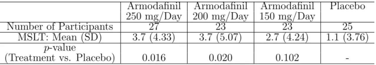
the estimated covariance for three-hypothesis testing givenα= 0.025 (10,000 simulations). . . 38 2.7 Multiple Sleep Latency Test change from baseline in 4 groups. . . 40 3.1 Familywise error rate of inverse normal method in multivariate case

given α= 0.025 (100,000 simulations). . . 56

correlation under different sample size given τ = 0.5,π1 = 0.0026 and

α= 0.025 (100,000 simulations). . . 58 3.3 Maximum sample size for two-stage GSD with two primary endpoints

to reach 90% power at one-sided overall significance levelα = 0.025. . 61 3.4 Power comparisons given n = 200, µ2 = 0.2, α = 0.025 and interim

time τ = 0.5 (10,000 simulations). . . 65 3.5 Maximum sample size and average sample size comparisons given power of

90%, ρ = 0.5, µ2 = 0.2, π1 = 0.0014, α = 0.025 and interim time τ = 0.5

(10,000 simulations). . . 67 3.6 Power of rejecting both endpoints simultaneously given n= 200, µ2 =

0.2, α= 0.025 and interim time τ = 0.5 (10,000 simulations). . . 69 4.1 Critical Values for comparing K treatment arms against control group

in one-sided Dunnett test. . . 77 4.2 Critical Valuesατ,K for the traditional pick-the-winner design with K

treatment arms. . . 79 4.3 Critical Values α∗_τmax,K for DLDGKP. . . 81 4.4 Optimalτmax with the corresponding critical Valuesα∗τmax,K for DLDGKP. 81 4.5 Response curves of treatment groups for efficacy and toxicity endpoints. 86 4.6 Sample sizes used for different number of treatment arms. . . 86

ment arms. . . 87 4.8 Operating characteristics of DLDGKP without and with adjustable

sample size. . . 89 4.9 Comparisons between DLDDunnett and DLDGKP using utility function

and traditional Pick-the-Winner designs. . . 91 E.1 Familywise error rate for two-hypothesis testing using SPPM given

α= 0.025. . . 127 E.2 Familywise error rate for three-hypothesis testing using SPPM given

α= 0.025. . . 127 F.1 Familywise error rate using SPPM procedure with the estimated

covari-ance for two-hypothesis testing given α= 0.025 (100,000 simulations). 128 H.1 Power comparisons given n = 200, µ2 = 0.2, α = 0.025 and interim

time τ = 0.5 (10,000 simulations). . . 132 H.2 Power of rejecting both endpoints simultaneously given n= 200, µ2 =

0.2, α= 0.025 and interim time τ = 0.5 (10,000 simulations). . . 134 J.1 Familywise error rate of DLDGKP using utility function givenα= 0.025

(100,000 simulations). . . 139

1·1 Graphical illustration of the weighted Bonferroni-Holm procedure with two and three hypotheses (Bretz et al., 2009). . . 9 4·1 Power comparisons between DLDDunnett and DLDGKP for different

number of treatment arms. . . 88 A·1 FWER under the global null hypothesis with the different correlations. 99 C·1 Integral region of π1₃. . . 106 C·2 Integral region of π2 3. . . 107 C·3 Integral region of π3 3. . . 108 C·4 Integral region of π1₃₁. . . 109 C·5 Integral region of π2 31. . . 110 C·6 Integral region of π3 31. . . 111 C·7 Integral region of π1₁₂₃. . . 112 C·8 Integral region of π2 123. . . 113 xvi

4A . . . Adaptive Alpha Allocation Approach CDF . . . Cumulative Distribution Function DLD . . . Drop-the-Loser Design

DLDDunnett . . . Drop-the-Loser Design with Dunnett critical value DLDGKP . . . Drop-the-Loser Design with GateKeeping Procedure GSD . . . Group Sequential Design

GSMulti . . . GSD using Multivariate Normal Distribution GSMulti v . . . GSMulti using Reallocating Significance Level IUT . . . Intersection-Union Testing

MTTR . . . Maximum Tolerated Toxicity Rate OBF . . . O’Brien Fleming stopping Boundary PDF . . . Probability Density Function

PWD . . . Pick-the-Winner Design

SPPM . . . Single Parametric Progressive Multiple Testing UIT . . . Union-Intersection Testing

Chapter 1

Introduction

1.1

Multiple Testing Procedures

Multiplicity issues arise prevalently in a variety of situations in clinical trials, and statistical methods for multiple testing have gradually gained importance with the increasing number of complex clinical trial designs. A proper treatment of multi-plicity issues is a key component of a well-controlled clinical trial. In general, two types of multiple testing can be performed (Dmitrienko et al., 2009). One is the union-intersection testing (UIT), which is expressed as an intersection of a family of hypotheses. The global null hypothesis in the UIT framework is rejected if at least one of its individual null hypotheses is rejected. Carrying out the individual tests at an unadjusted level leads to an inflation of the probability of rejecting the global null hypothesis. To address this issue, an adjustment to a smaller value of significance level for testing each individual hypothesis or a modification of testing procedure needs to be utilized. Another type is the intersection-union testing (IUT), which, in contrast to UIT, can be expressed as the union of a family of hypotheses. The global null hypotheses is rejected if each of its individual null hypotheses is rejected.

No multiplicity adjustment is necessary to control the size of the test in this testing. Other multiple hypothesis testing can be in the form of the combination of these two frameworks.

In union-intersection testing, the hypothesis testing can be formulated as:

H0 : ∩Kk=1µk≤0(∩Kk=1Hk) v.s Ha: ∪Kk=1µk>0(∪Kk=1H¯k),

where Hk and ¯Hk are the null and alternative hypotheses for the kth test. The

probability of making at least one type I error in UIT increases with the number of individual hypotheses tested. To solve this problem, the probability of falsely rejecting at least one null hypothesis, which is defined as familywise error rate (FWER), is required to be controlled in the strong sense, especially in confirmatory clinical trials. Using the mathematical terminology, this requirement is to control the probability of incorrectly rejecting any true hypothesis regardless of which and how may other hypotheses are true. In the formulation, if T is the index set of true null hypotheses, then:

supF W ER= max

T supP r(k ∈T : Reject at least one Hk)≤α,

where the supremum is taken over all parameters µk in the null hypothesis space for

k ∈T and in the alternative hypothesis parameter space fork 6∈T, and the maximum is taken over all index sets T. In this way, the FWER is controlled in the strong sense.

A number of methods have been developed and introduced for controlling the FWER within the acceptance limit, including single-step and stepwise procedures. In

single-step approaches, the unadjusted p-values are compared to the adjusted local significance level to make the rejection decision about the global null hypothesis, or the adjusted p-values are used to compare against the unadjusted significance level.

Bonferroni Method

The common used and simple method is Bonferroni method. The adjusted test level alpha αk for each hypothesis is stated as αk = _Kα. This is a conservative single-step

approach without consideration of any correlations among p-values. The alpha level can also be split unequally, in which the adjusted alpha level is: αk = wkα, where

the weights PK

k=1wk = 1. This weightswk can be determined based on the clinical

importance or the power of the kth _{hypothesis. This approach is called weighted}

Bonferroni method.

Fisher Combination Test

Fisher combination test is usually used to test the global null hypothesisH0, in which

the Fisher statistic is:

χ2 =−2

K

X

k=1

ln(pk),

where pk is the univariatep-value for testingHk. If the test statistics are independent,

then χ2 _{is distributed as a chi-square distribution with 2K degrees of freedom under}

H0, and the global nullH0 is rejected ifχ2 ≥χ22K,1−α.

Single-step approaches can be improved in terms of power through stepwise approaches, while also controlling for the desired error rate. With stepwise approaches, some hypotheses may be retained or rejected by implication of decisions about other

hypotheses. Stepwise approaches can be applied via step-down and step-up procedures. A compromise between the Holm and the fixed-sequence procedures can be obtained by the fallback procedure introduced by Wiens (Wiens, 2003).

Hommel Step-Up Procedure

A step-up procedure starts with the least significant p-value. Assume p(1), . . . , p(K) are

the sorted p-values for K hypotheses in the increasing order, with the corresponding hypotheses as H(1), . . . , H(K). Hommel procedure follows algorithm as:

• If p(K) > α, retain H(K) and go to the next step, otherwise, reject all hypotheses

and stop.

• For k= 2, . . . , K −1, if p(K−j+1) >(k−j+ 1)α/k forj = 1, . . . , k, retain H(K−k+1)

and go to the next step. Otherwise reject all remaining hypotheses and stop.

• Ifp(K−j+1) >(k−j + 1)α/k forj = 1, . . . , K, retainH(1), otherwise reject it.

Hochberg Step-Up Procedure

The Hochberg procedure is another popular step-up procedure, and the decision rule for the Hochberg procedure is as follows:

• If p(K) > α, retain H(K) and go to the next step. Otherwise reject all hypotheses

and stop.

• For k = 2, . . . , K −1, if p(K−j+1) > α/k, retain H(K−k+1) and go to the next step.

Otherwise reject all the remaining hypotheses and stop.

• Ifp(1) > α/K, retain H(1). Otherwise reject it.

When only two individual hypotheses are involved in the multiple testing, Hochberg and Hommel provides the same decisions.

Holm Step-Down Procedure

A step-down procedure starts with the hypothesis associated with the most significant

p-value. In general, the Holm procedure examines hypotheses in the sequence as:

• Ifp(1) ≤α/K, reject H(1) and go to the next step. Otherwise retain all hypotheses

and stop.

• For k = 2, . . . , K−1, if p(k) ≤α/(K −k+ 1), reject H(i) and go to the next step.

Otherwise retain all remaining hypotheses and stop.

• Ifp(K)≤α, reject H(K). Otherwise, retain H(K).

Fallback Procedure

The fixed-sequence procedure assumes that the order in which the hypotheses are tested is pre-specified and testing begins with the first hypothesis and is carried out without a multiplicity adjustment if the results are significant in all preceding tests. For the fallback procedure, the hypotheses are ordered first as well (H1, . . . , HK) and

the overall test level αis split among the hypotheses by the weights w1, . . . , wK. Then

the procedure is as follows:

• Ifp1 ≤w1α, reject H1 otherwise retain it. Then go to the next step.

• For k= 2, . . . , K, testHk atαk =αk−1+wkα if Hk−1 is rejected andαk=wkα if

Hk−1 is retained. If pk ≤αk, reject Hk otherwise retain it.

However, all the aforementioned methods do not take into account the joint distribution of the test statistics; therefore they might suffer power loss when the correlation exists. It is possible to improve the power by utilizing the known or assumed joint distribution of the test statistics, which is called a parametric procedure.

The most well-known parametric procedure was developed by Dunnett (Dunnett, 1955) for the dose-response design. In the adaptive alpha allocation approach (4A) by Li and Mehrotra (Li and Mehrotra, 2008), the hypotheses are grouped into two families on the basis of previous trial power and allows the significance level for the second underpowered family to be set adaptively based on the largest observedp-value in the adequately powered first family.

Dunnett Test

The Dunnett procedure is based on the joint distribution and thus accounts for the correlation among the test statistics, and it was originally developed for the multiplicity problems in multiple dose-control comparisons. Consider a multiple arm clinical trial comparing K doses or treatments to a control group, in which xkj is the response of

the jth individual in thekth treatment group,k = 0, . . . , K (where k= 0 denotes the control group). The t statistic for testing Hk is: tk = x¯k−¯x0

s √

2/n, with s as the pooled

sample standard deviation. The test statistic for testing global null is:

T =max

k tk. (1.1)

The multivariate t-distribution of T in Eq (1.1) is one-sided Dunnett distribution with degree of freedom ofν = (K+ 1)(n−1). The Dunnett critical value,µα =F−1(1−α),

is evaluated under the global null hypothesis, where F(x) is the CDF of Dunnett distribution. The individual hypothesis Hk is rejected if tk ≥ µα, k = 1, . . . , K.

Adaptive Alpha Allocation Approach

approach (4A), which is a data-driven approach. 4A controls the FWER at level

α and can notably increase the probability of achieving a positive trial compared with fixed prospective alpha allocation scheme. The research work discussed the testing procedures for the independent and correlated endpoints. For the independent endpoints, endpoint A is tested at the pre-specified level α1 =α−, and the endpoint

B is tested at the adaptive level:

α2(pA, α1, α) = α, if pA≤α1; min(αt p2 A, α1), if pA> α1, where αt= ( α1(1− q 2α1−α−α21 α1 ) 2_{, if α} 1+α21−α 3 1 ≤α; α1α−α_1−α11, if α1+α21−α 3 1 > α,

The extension to three or more independent primary endpoints is also discussed, where the tests for the type A endpoints are tested at level α1 using any multiplicity

adjustment procedure, such as Hommel or Hochberg methods. The p-values for the type B primary endpoints are then assessed at an adaptive overall level based on the observed largest p-value for type A endpoints using multiplicity adjustment procedure. The adaptation method for the correlated primary endpoints is also available in (Li and Mehrotra, 2008).

Recently, more advanced testing approaches have been introduced. The gatekeeping approach based on the closure principle (Dmitrienko et al., 2006a) is an appropriate method in the situation when one family of hypotheses treated as a gatekeeper and

the other families are tested only if one or more gatekeeper hypotheses have been rejected. However, the gatekeeping procedure is difficult to communicate with the non-statisticians and requires large set of tests as the number of individual hypotheses increases. An iterative graphical approach (Bretz et al., 2009) deals with those weakness, and constructs the Bonferroni-type tests with a simple updating algorithm that fully describes a sequentially rejective test procedure. Bretz (Bretz et al., 2011) described these ideas with more details and further extensions, including weighted Bonferroni, Simes and parametric tests.

Graphical Approach

The iterative graphical approach is used to construct and perform Bonferroni-type tests, which is represented by directed and weighted graphs with visualized expression. Using a graphical approach, the hypotheses are represented by a set of vertices with local significance levels. The weight associated with a directed edge between any two vertices indicates the fraction of the significance level at the initial vertex that is added to the significance level at the terminal vertex, if the hypothesis at the initial vertex is rejected. Let α1, . . . , αK be the initial allocation of the overall significance level

for each hypothesis such as PK

k=1αk ≤α. Figure (1·1) shows the graphical approach

for two and three hypotheses. For two hypotheses testing in Figure (1·1.A), if H1 is

rejected at α1, the initially allocated significance level forH1 is passed to H2, then

H2 is tested at α. Vice versa, if H2 is rejected at α2, then H1 is tested at level α.

Similarly, Figure (1·1.B) shows the illustration for the three hypotheses with the equal initial significance level allocation and the equal edges of fraction recycling.

Figure 1·1: Graphical illustration of the weighted Bonferroni-Holm procedure with two and three hypotheses (Bretz et al., 2009).

1.2

Group Sequential Design

Group sequential designs (GSD) are clinical trials which allows interim looks with the possibility of early terminations due to efficacy, harm or futility, in such a way as to maintain a prescribed significance level and power against alternatives. Therefore, GSD can also help in reducing the overall costs and timelines for the development of a new drug. Repeated looks of data may inflate the Type I error rate due to multiple testings of interim analyses, and the proper treatments to the error inflation haven been discussed widespreadly. Simple group sequential approaches for a pre-specified number

of equally spaced interim analyses were developed (Pocock, 1977; O’Brien and Fleming, 1979) by adjusting the critical values to control the type I error. Wang and Tsiatis (Wang and Tsiatis, 1987) generalized Pocock and O’Brien and Fleming methods to a class of boundaries with a shape parameter. However, those approaches require the fixed maximum number of analyses with equally spaced interims and therefore lack in flexibility. Lan and DeMets (Lan and DeMets, 1983) proposed an alternative method of usingα-spending functions to construct discrete sequential boundaries, in which the boundary at each decision time is determined by the information time of the interim analysis. The Lan and DeMets approach has been extended to one-parameter family of α-spending functions in order to construct customized designs (Kim and DeMets, 1987; Hwang et al., 1990), and been generalized to futility test of interim analyses using type II error spending function (Pampallona et al., 2001). The spending function approach has become popular because of its flexibility in allowing unequally spaced interim analyses and some room for changing the interim analyses on the condition of no knowledge of treatment effects. Most literature about GSD focuses on a single endpoint, however, GSD with multiple endpoints has also received considerable attention.

Pocock Boundary

Pocock (Pocock, 1977) proposed to perform a test at a constant nominal level at each interim analysis. Suppose a group sequential design with M planned repeated looks, and Zm is the test statistic at mth stage. LetCp(M, α) be the Pocock stopping

• In the mth _{stage (m = 1, . . . , M −1), if |Z}

m|> CP(M, α), then stop the trial and

reject H0; otherwise continue to the (m+ 1)th stage.

• In the last stage, if |ZM|> CP(M, α), then stop the trial and reject H0; otherwise

stop and accept H0.

O’Brien and Fleming Boundary

Contrast to Pocock’s test, O’Brien and Fleming (O’Brien and Fleming, 1979) suggested a test by increasing the nominal significance level for each stage analysis, which makes it difficult to reject the null hypothesis at the early stage of the trial. The OBF test is as follows:

• In the mth _{stage (m = 1, . . . , M −1), if |Z}

m|> COBF(M, α)

p

M/m, then stop the trial and rejectH0; otherwise continue to the (m+ 1)th stage.

• In the last stage, if|ZM|> COBF(M, α), then stop the trial and reject H0; otherwise

stop and accept H0.

Error Spending Function Approach

The error spending function was proposed to offer more flexibility of study design. Let

τ denote the information time during the course of a clinical trial, where τ = n/N, n

is the accumulative sample size at the time of interim analysis and N is the target sample size. The alpha spending function,α(τ), is a monotonically increasing function. At the beginning of trial (τ = 0), α(τ) = 0; and at the end of trial (τ = 1),α(1) =α, which is the overall significance test level. Once an interim analysis is performed, part of the overall alpha is spent for testing. For the interim analysis at the information time of τ, α(τ) determines the probability of any of the interim analyses before τ

leading to rejection of the null hypothesis when the null hypothesis is true. The stopping boundary requires numerically integrating the distribution function.

1.3

Drop-the-Loser Design

A drop-the-loser adaptive design (DLD) is useful in phase II and sometime phase III clinical development especially when there are uncertainties regarding the dose levels. Usually, in the first stage of a two-stage DLD, the candidates for the best treatment based on the efficacy are selected. At the second stage, additional observations are collected in those candidate arms and control arm to decide whether the candidate is actually better than the control. DLDs allow for multiple treatment arms with the opportunity to more fully characterize the dose-response during the initial phase of the trial. An interim analysis plan specifies the criteria for dropping doses/treatments that fail to show clinically meaningful efficacy over placebo. The doses/treatments satisfying interim efficacy criteria are continued to completion. This adaptive pruning permits the randomization of remaining participants to the conditions which demonstrate the most encouraging performance.

Pick-the-Winner Design

The straightforward example of DLD is a two-stage pick-the-winner which only allows one winner arm selected in the interim stage carried to the final stage (Chang, 2014). Suppose a trial starts with K treatment arms and one control arm. The sample size for each group is N, and the interim analysis will perform at the information time τ = N1

and the control arm will be carried and additional N2 =N −N1 individuals in each

arm will be recruited. Let ¯xk be the mean of the first stage data for the kth arm

(k = 0,1, . . . , K), and ¯yk be the mean of the incremental second stage data from

N(µk, σ2), where k = 0, S, and arm S is the treatment arm selected in the interim.

Let tk = x¯_σk √

N1 and τk= y¯_σk √

N2 be the stagewise test statistics, respectively. Then

the maximum statistic at the end of the first stage is T1 = max(t1, . . . , tK), with the

pdf as fT1(t) =K[Φ(t)]

K−1_{φ(t). Let δ}

k = 1 whenk =S, otherwise δk = 0. Then the

cdf of the statistic T2 for the winner arm in the final stage is:

FT2(t) = K X k=1 P(δk= 1∩T1 √ τ +τi √ 1−τ < t). (1.2)

The final test statistic is defined as: T₂∗ = (T2−t0)/ √

2, with the pdf as:

FT∗ 2(z) = Z ∞ −∞ FT2(t)φ( √ 2z−t)dt. (1.3)

The stopping boundary can be derived from Eq. (1.3) by solving FT∗

2(z) = 1−α. This

design only allows to reject H0 at the final analysis. Additionally, a lot of different

DLD designs are existing which have diversified dropping arms manners as long as the criterion is defined in the beginning of the trial.

1.4

Dissertation Outline

In this dissertation, we study the multiple testing problems in the classical clinical trials and adaptive designs, and develop the novel testing procedures to solve the

multiple testing problems in the different study design. The complete methods and the corresponding simulation studies are presented in each chapter.

In Chapter 2, we develop a single-step progressive parametric multiple (SPPM) testing procedure, which considers the joint distribution of the test statistics. The procedure constructs the testing using the products of all the combinations of local individual p-values and the critical values are determined by numerical integrations progressively using the closure principle. The performance of the SPPM has been compared through extensive simulations to several other existing multiple testing procedures, which demonstrate the advantage of using the SPPM procedure, in terms of power, for the certain situations of multiple testing. The method can also take the clinical importance and/or statistical power into consideration when distributing the error rate among the individual hypotheses. An application of SPPM to a Phase III dose-finding trial is also presented.

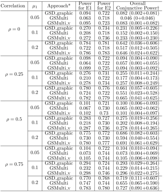
In Chapter 3, an intuitive approach is proposed, which utilizes the multivariate normal distribution to deal with multiplicity issues arising from multiple endpoints and from multiple looks in group sequential design. The approach is a closed testing procedure, and therefore it controls the familywise error rate in a strong sense. The procedure could also have various applications in other designed trials, such as biomarker design and multiple-arm design. In addition, we discuss the alpha-reallocation to improve the conjunctive power of rejecting all endpoints with the FWER controlled for special requirements in the clinical trial designs. Through extensive simulations, the proposed method is demonstrated to gain the power compared to the

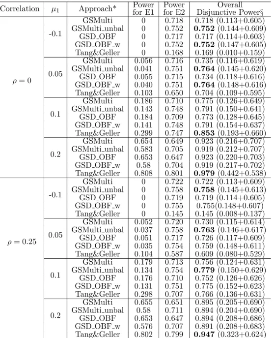
Bonferroni correction for multiple primary endpoints in group sequential designs when the correlation among endpoints exists and has some power advantages compared to the Tang and Geller method when the effect sizes differ.

In Chapter 4, we propose the flexible drop-the-loser designs based on the traditional Dunnett test and the pick-the-winner design in the gatekeeping testing manner, both of which allow more flexibility of treatment selections without pre-specified mechanism and still retain acceptable power. The simulation study is conducted for different combinations of efficacy and safety response curves using two flexible DLD designs, and the power performance shows different patterns for two methods according to the response curves. In addition, the drop-the-loser design in the gatekeeping testing manner is explored with the adjustable sample size in the interim if the winner arm based on the efficacy data is discontinued due to the safety issue. The utility function, as a measurement of balance between efficacy and toxicity, is also included as the criterion of treatment selection for the two methods.

The three topics in the chapters are introduced to solve the multiple testing problems in different study design: SPPM testing procedure is proposed to improve the power for union-intersection testing problem, which can be applied in the multiple primary endpoints design, multiple arm design in the classical clinical trial; GSMulti procedure is designed to improve the power of multiple primary endpoints in GSD, where the multiplicity problem comes from endpoints and repeated looks; the two extension methods of drop-the-loser design (DLD) is developed to improve the power in the multiple arm adaptive designs, and the multiplicity comes from pairwise

comparisons among arms. These three projects show the importance of correlation in the multiple testing procedures. The critical values of SPPM and GSMulti are derived based on the correlation and both two methods demonstrate the advantage of utilizing the correlation in terms of boosting power. For DLD designs, the critical values are based on Dunnett test, where the joint distribution of test statistics are considered when deriving the critical values as well. In summary, my dissertation is dealing with the multiplicity issues in general, and the information about correlation could be used when we design a trial.

Chapter 2

Single-Step Progressive Parametric

Multiple Testing Procedure for Correlated

Normal Test Statistics

2.1

Introduction

In general, multiplicity is from the simultaneous evaluation of different aspects of the efficacy or safety profile of a treatment (Dmitrienko et al., 2013).The statistical methods for multiple testing have gradually gained importance with the increasing number of complex clinical trial designs.

Two types of global multiple hypotheses testing can be performed (Dmitrienko et al., 2009): union-intersection testing (UIT) and intersection-union testing (IUT). We focus on the UIT framework in the dissertation. The null hypothesis of UIT is an intersection hypotheses, and the global null hypothesis is rejected if at least one of its individual null hypotheses is rejected. In UIT framework, the familywise error rate (FWER) - the probability of falsely rejecting at least one null hypothesis - is required to be controlled in the strong sense at level α, which means FWER≤α in

spite of which other hypotheses are true. A modification of testing procedure needs to be done to control the error strongly. A number of methods have been developed for controlling the FWER within the acceptance limit, including single-step and stepwise procedures. In single-step approaches, such as the simple Bonferroni method and the Sidak method (ˇSid´ak, 1967), the rejection decision of a hypothesis does not depend on the decision of any other hypotheses. Single-step approaches can be improved in terms of power through stepwise approaches, while also controlling for the desired error rate. With stepwise approaches, some hypotheses may be retained or rejected by implication of decisions about other hypotheses. Stepwise procedures include the Holm stepdown method (Holm, 1979), the Hochberg step-up procedure (Hochberg, 1988) and the Hommel step-up procedure (Hommel, 1988) and so on. The fixed-sequence testing approach (Maurer et al., 1995), (Westfall et al., 2011) is also one category of stepwise procedure that assumes the order in which the hypotheses are tested is pre-specified before the data collection. A compromise between the Holm and the fixed-sequence procedures can be obtained by the fallback procedure introduced by Wiens (Wiens, 2003) and was further studied (Wiens and Dmitrienko, 2005), (Dmitrienko et al., 2006b). When the adjustedp-value for each hypothesis is found based on the collected data, the stepwise procedure is simplified to the situation that the adjusted p-values are compared against significance α level in any testing order.

However, it is also possible to improve the power by utilizing a parametric procedure with the known or assumed joint distribution of the test statistics. The most well-known parametric procedure was developed by Dunnett (Dunnett, 1955) for the

dose-response design. The stepwise version of Dunnett procedure (Marcus et al., 1976), (Dunnett and Tamhane, 1992) can boost power compared to the single-step one. Huque and Alosh (Huque and Alosh, 2008) proposed a flexible fixed-sequence testing procedure, which takes into account correlations among endpoints for higher flexibility. In the adaptive alpha allocation approach (4A) by Li and Mehrotra (Li and Mehrotra, 2008), the hypotheses are grouped into two families on the basis of previous trial power and allows the significance level for the second underpowered family to be set adaptively based on the largest observed p-value in the adequately powered first family. Li et al. (Li et al., 2013) generalized 4A and used well-defined functions of the joint distribution of multiple endpoints to calculate the alpha allocation for the second family. Some advanced testing approaches also have been introduced. An iterative graphical approach (Bretz et al., 2009) constructs the Bonferroni-type tests with an updating algorithm that fully describes a sequentially rejective test procedure, which is easier to communicate to the non-statisticians. Bretz (Bretz et al., 2011) described these ideas with further extensions, including the parametric tests.

Littell and Folks (Littell and Folks, 1971), (Littell and Folks, 1973) showed that the Fisher’s combination test (Fisher, 1932) is asymptotically optimal among essentially all methods of combining independent tests. The extensions of the Fisher’s combination test allowing the dependent tests are available for both completely specified covariance matrix (Brown, 1975) and partially defined covariance matrix with a known scalar quantity (Kost and McDermott, 2002). However, those product combination tests are global tests and control the FWER only when all null hypotheses are true, thus,

provide weak control of the FWER. There are a number of applications of Fisher’s method in the adaptive designs as well (Bauer and Kohne, 1994), (Wassmer, 1999), (Hommel et al., 2005), (G¨otte et al., 2009), (Schmidt et al., 2014). Based on Fisher’s method, Bauer and K¨ohne (Bauer and Kohne, 1994) designed a two-stage adaptive design controlling the FWER in the strong sense, which was also considered forK >2 stages design (Wassmer, 1999). Hommel et al. (Hommel et al., 2005) proposed the modified Simes test for a two-stage adaptive design with correlated test statistics, and G¨otte et al. (G¨otte et al., 2009) extended MST and generalized (Bauer and Kohne, 1994) for correlated test statistics. In this chapter, we propose a straightforward but powerful single-step progressive parametric multiple (SPPM) testing procedure using the product combination as well and taking the correlation into account. The procedure constructs the testing using the products of all the combinations of local individual

p-values as well, and the critical values are determined by numerical integrations progressively using the closure principle, therefore, the procedure can strongly control the FWER. It also allows the possibility of different allocation of significance level

α according to the effect sizes or the clinical importance. The simulation studies demonstrate our procedure improves power substantially when the correlation is moderate and the difference in the effect sizes is small.

This chapter evolves as follows. We begin with a description of the proposed single-step progressive parametric multiple testing procedure in two-hypothesis testing and the critical values are derived mathematically using numerical integration, followed by the extension to three-hypothesis. The extensive simulation studies demonstrate

that in most situations the proposed procedure is more powerful than the current broadly used methods. The “Discussion” section concludes the topic with a short summary and discussion of future potential work.

2.2

Single-step Progressive Parametric Multiple Testing

Pro-cedure

2.2.1 Two-Hypothesis Testing Procedure

First, we discuss the situation of two one-sided test hypotheses in the UIT framework:

H0 : µ1 ≤0∩µ2 ≤0(H1∩H2) v.s Ha: µ1 >0∪µ2 >0( ¯H1∪H¯2), (2.1)

where Hk and ¯Hk are the null and alternative hypotheses for thekth test (k = 1,2),

respectively. The single-step progressive parametric multiple (SPPM) testing procedure is performed as follows:

• Ifp1p2 ≤α1 and p1 ≤α0, reject H1; • Ifp1p2 ≤α2 and p2 ≤α0, reject H2,

wherepkis the univariate localp-value forHk, andαk0sare the critical values. According

to the closure principle, a hypothesis is rejected if all intersection hypotheses containing this hypothesis are rejected, and testing each intersection hypothesis using a local

to control the error rate at α under H1 and H0. Therefore, we have: P r1 = sup µ1∈H1 Pr(RejectH1|H1) = sup Pr(p1p2 ≤α1∩p1 ≤α0|H1)≤α; P r2 = sup µ2∈H2 Pr(RejectH2|H2) = sup Pr(p1p2 ≤α2∩p2 ≤α0|H2)≤α; P r0 = sup µ0 ks∈H0

Pr(Reject at least one Hk|H0)

= Pr(p1p2 ≤α1∩p1 ≤α0|H0) + Pr(p1p2 ≤α2∩p2 ≤α0|H0) −Pr(p1p2 ≤min(α1, α2)∩p1 ≤α0 ∩p2 ≤α0|H0)≤α.

It is easy to obtain that α0 ≤ α from P r1 or P r2, and α0 = α is used to exhaust

α and improve the power. Moreover, we also see the idea behind this procedure is to borrow strength among the marginal p-values, that is, there is no need to make an α adjustment to reject H1 as long as p1 ≤ α and p2 is small. Afterwards, the

critical values α1 and α2 are determined by controlling P r0 atα. Our SPPM testing

procedure has both coherence and consonance properties. It is coherent due to the closure principle, and is consonant because rejecting an intersection hypothesis Hi

will lead to the rejection of at least one Hk implied by Hi. In addition, the rejection

decision of Hk in SPPM testing procedure depends on the observed data from other

hypotheses, however, it is a single-step testing procedure because the rejection or non-rejection of a single hypothesis Hk does not depend on the decision on any other

hypothesis. Therefore, the proposed procedure can test hypotheses simultaneously or in any order. It can be shown by the extensive simulations that the worst case

under the global null is when all µ0_ks equal to 0 (see Appendix A for details). Then

P r0 is simplified as P r(Reject at least one Hk)≤α under H0∗: µ1 = µ2 = 0, and this

simpler and more convenient condition is used for derivations of critical values. Here, we assume that the test statistic for the kth _{hypothesis is Z}

k ∼ N(µk,1)

with univarite p-value pk, then pk follows Uniform(0,1) under Hk. The correlation

between Z1 and Z2 is denoted by ρ. By the property of the multivariate normal

distribution (Eaton, 1983), the conditional distribution of Z2, given Z1 = z1, is

N(µ2+ρ(z1−µ1),1−ρ2). Then, the conditional cumulative density function (CDF)

for p1p2 givenp1, under H0∗, is:

Pr p1p2|p1 (p1p2 ≤α1|p1) = Pr(p2 ≤ α1 p1 |p1) =    1, α1 p1 ≥1; Pr(Z2 ≥Φ−1(1− _1−Φ(zα1 ₁₎)|Z1 =z1) = 1−g(p1), α1 p1 ≤1. where we define g(x) := Φ((Φ−1(1− α1 x )−ρΦ −1_(1−x))/p

1−ρ2_{). The type I error}

rate for H1 under H0∗ is:

Pr(p1p2 ≤α1∩p1 ≤α|H0∗) = Pr(p1 ≤α|H0∗), α1 ≥α; Rα 0 P rp1p2|p1(p1p2 ≤α1|p1)f(p1)dp1, α1 < α. = α, α1 ≥α; α−Rα α1g(p1)dp1, α1 < α. (2.2)

The type I error rate for H2 underH0∗: Pr(p1p2 ≤α2∩p2 ≤α|H0∗) can be derived in

a similar manner. Next, the probability of rejecting two hypotheses simultaneously should be obtained in the two situations defined by the value of min(α1, α2). When

α2 _≤min(α

1, α2), we have:

Pr(p1p2 ≤min(α1, α2)∩p1 ≤α∩p2 ≤α|H0∗) = Pr(p1 ≤α∩p2 ≤α|H0∗)

= Pr(Z1 ≥Φ−1(1−α)∩Z2 ≥Φ−1(1−α)|H0∗) =:FZ,

When α2 _>min(α

1, α2) =α1, the probability becomes:

Pr(p1p2 ≤α1 ∩p1 ≤α∩p2 ≤α|H0∗) = Z α_α1 0 Pr(p2 ≤α|p1)dp1+ Z α α₁ α Pr(p2 ≤ α1 p1 |p1)dp1 =α−( Z α_α1 0 h(p1)dp1+ Z α α₁ α g(p1)dp1),

where we define h(x) := Φ((Φ−1(1−α)−ρΦ−1(1−x))/p1−ρ2_{).When min(α}

1, α2) =

α2, the probability of rejecting two hypotheses simultaneously can be written in the

P1 = sup µ1∈H1 Pr(RejectH1|H1)≤α; P2 = sup µ2∈H2 Pr(RejectH2|H2)≤α; P0 = sup µk∈H0

Pr(Reject at least oneHk|H0) =

                   2α−FZ, α≤α1 ≤α2; 2α−Rα α1g(p1)dp1−FZ, α 2 _≤α 1 < α≤α2; 2α−Rα α1g(p1)dp1− Rα α2g(p2)dp2−FZ, α 2 _≤α 1 ≤α2 < α; α−Rα α1g(p1)dp1+ R α_α1 0 h(p1)dp1+ Rα α₁ α g(p1)dp1, α1 < α2 < α≤α2; α−Rα α1g(p1)dp1− Rα α2g(p2)dp2+ Rα_α1 0 h(p1)dp1+ Rα α₁ α g(p1)dp1, α1 < α2 and α2 < α. (2.3)

The critical values α1 and α2 are determined by satisfying P0 ≤α in Eq. (2.3).

How-ever, the condition α≤αk is not viable because there is no solution between 0 and

1 and p1p2 ≤ αk in the testing procedure actually no longer has any effect for this

condition. In the simple case of α1 =α2, we have:

2α−2

Z α

α1

g(p1)dp1−FZ(Φ−1(1−α),Φ−1(1−α))≤α, α2 ≤α1 =α2 < α. (2.4)

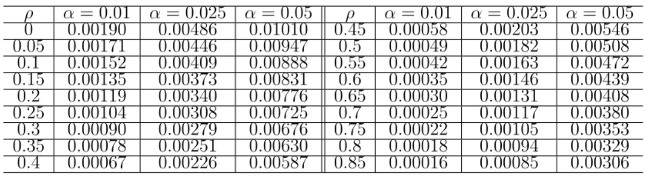
The critical values α1 = α2 for a one-sided test under different correlations given

various significance levelα are shown in Table 2.1. 100,000 simulations also succeeded to verify that the critical values derived mathematically strongly control the FWER as shown in Appendix E. From Table 2.1, the critical values are decreasing with the increase in correlation, which indicates the most conservative condition for SPPM

given the multivariate normal distribution of test statistics with known covariance matrix is when the two test statistics are perfectly correlated (ρ= 1). If the correlation is not considered and the critical values with ρ= 0 is used, the FWER will be inflated especially when the true correlation is strong. For practical use, the critical value α1

for the test with a correlation that is not listed in Table 2.1 can be obtained using a linear interpolation; or, a conservative value can be used. For example, if α= 0.025 and correlation ρ= 0.08, the critical value of 0.004085 for ρ = 0.1 could be chosen. We also provided the R functions in Appendix B to calculate the critical values for all the situations ofα1 and α2.

Table 2.1: Critical values of one-sided test for two-hypothesis test with different correlations when α1 =α2.

ρ α= 0.01 α= 0.025 α = 0.05 ρ α= 0.01 α= 0.025 α = 0.05 0 0.00190 0.00486 0.01010 0.45 0.00058 0.00203 0.00546 0.05 0.00171 0.00446 0.00947 0.5 0.00049 0.00182 0.00508 0.1 0.00152 0.00409 0.00888 0.55 0.00042 0.00163 0.00472 0.15 0.00135 0.00373 0.00831 0.6 0.00035 0.00146 0.00439 0.2 0.00119 0.00340 0.00776 0.65 0.00030 0.00131 0.00408 0.25 0.00104 0.00308 0.00725 0.7 0.00025 0.00117 0.00380 0.3 0.00090 0.00279 0.00676 0.75 0.00022 0.00105 0.00353 0.35 0.00078 0.00251 0.00630 0.8 0.00018 0.00094 0.00329 0.4 0.00067 0.00226 0.00587 0.85 0.00016 0.00085 0.00306

2.2.2 Three-Hypothesis Testing Procedure

The null and alternative hypotheses for three hypotheses are written as:

where Hk and ¯Hk are the null and alternative hypothesis for the kth test (k = 1,2,3),

respectively. Analogous to the two-hypothesis testing procedure in Section 2.2.1, the SPPM procedure is conducted as:

• If p1p2p3 ≤α4, pipj ≤ αi and pipj0 ≤ α_i and p_i ≤α₀, reject H_i; otherwise, accept

Hi;

where i, j, j0 = 1,2,3, i6=j 6=j0, and the critical values are α1, . . . , α4. According to

the closure principle, each hypothesis below is tested at α-level:

           P ri = sup µi∈Hi Pr(RejectHi|Hi)≤α, P rij = sup µi,µj∈Hi∩Hj Pr(Reject either Hi orHj|Hi∩Hj)≤α, P r0 = sup µ0_is∈H0

Pr(Reject at least one Hi|H0)≤α,

(2.6)

where P ri and P rij(i, j = 1,2,3, i6=j) have the same formulations as the FWERs

un-der single hypothesis testing and two-hypothesis testing, respectively (see Appendix C for details). We again have α0 =α to use up α and maximize the power. The equal

pairwise correlations among three test statistics are assumed for now andα1 = α2 =α3,

the critical values in Table 2.1 can be used for α0_ks (k = 1,2,3) here. Given α0_ks,

α4 is determined progressively by solving P r0 = α. However, when the pairwise

correlations differ, the assumption of α1 = α2 = α3 can no longer be valid and the

critical values should be derived according to Eq. (2.6) one step by one. The critical values α4 for the three-hypothesis testing under various α and the equal pairwise

correlation ρ are listed in Table 2.2. The first line in each cell is the critical values

in some situations, which indicates no need for the criterion of p1p2p3 ≤α4 and the

FWER can be controlled implicitly by the other criteria. The R functions for the critical values in three-hypothesis testing assuming the equal pairwise correlation is also provided in Appendix D.

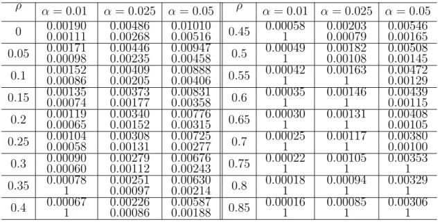
Table 2.2: Critical values of one-sided test for three-hypothesis test with different correlations (α1 =α2 =α3).

ρ _{α= 0.01 α= 0.025 α = 0.05} ρ _{α= 0.01 α= 0.025 α = 0.05} 0 0.00190_0.00111 0.00486_0.00268 0.01010_0.00516 0.45 0.00058₁ 0.00203_0.00079 0.00546_0.00165 0.05 _0.000980.00171 0.00446_0.00235 0.00947_0.00458 0.5 0.00049₁ 0.00182_0.00108 0.00508_0.00145 0.1 _0.000860.00152 0.00409_0.00205 0.00888_0.00406 0.55 0.00042₁ 0.00163₁ 0.00472_0.00129 0.15 _0.000740.00135 0.00373_0.00177 0.00831_0.00358 0.6 0.00035₁ 0.00146₁ 0.00439_0.00115 0.2 _0.000650.00119 0.00340_0.00152 0.00776_0.00315 0.65 0.00030₁ 0.00131₁ 0.00408_0.00105 0.25 _0.000580.00104 0.00308_0.00131 0.00725_0.00277 0.7 0.00025₁ 0.00117₁ 0.00380_0.00100 0.3 _0.000600.00090 0.00279_0.00112 0.00676_0.00243 0.75 0.00022₁ 0.00105₁ 0.00353₁ 0.35 0.00078₁ 0.00251_0.00097 0.00630_0.00214 0.8 0.00018₁ 0.00094₁ 0.00329₁ 0.4 0.00067₁ 0.00226_0.00086 0.00587_0.00188 0.85 0.00016₁ 0.00085₁ 0.00306₁

For example, when α = 0.01 and ρ = 0, the critical values α1 = α2 = α3 = 0.0019, and

α4= 0.00111.

2.3

Simulation Study

The emerging approaches dealing with the multiplicity problems have not shown substantial power improvement for a long time. In this section, the proposed SPPM testing procedure is compared to several popular approaches through extensive

simula-tions and is established to be more powerful when having similar effect sizes and small or moderate correlation. The power of the situation with the differential effect sizes can also be improved by modifying the critical values for two- and three-hypothesis testing procedures. We also investigated the FWER with estimated covariance matrix when the correlation and variance are unknown and showed the SPPM testing procedure can control the FWER strongly.

2.3.1 Power Comparisons of Two-Hypothesis Testing

We first study the performance of SPPM in terms of power compared to other methods in the two-hypothesis framework. The nonparametric testing procedures, including single-step and stepwise procedures, and the parametric testing procedure are evaluated together. The Bonferroni test is compared as a benchmark for the evaluation of power improvement. We also includes the Hochberg and Hommel procedures, the fallback procedure, the step-up Dunnett procedure and 4A method for comparison as well.

The FWERs of the existing methods are shown to be controlled well under the situations of the positively dependent test statistics, although some testing procedures could be conservative with strong correlations; the proposed SPPM procedure is derived under strong control of the FWER and was also verified by simulations to control the FWER (see Appendix E). Therefore, the power can be investigated directly on the same significance level at α= 0.025. The two correlated endpoints with sample sizeN as 90 were simulated and one-sample test was conducted with known covariance matrix. Based on 100,000 simulations, Table 2.3 shows the powers for four values of

known ρ: 0, 0.25, 0.5, 0.75, and three sets of effect sizes µ1 and µ2. Two different

types of power are shown here: the power of rejecting H1 andH2 at the same time,

denoted as Power1 and the power of rejecting either H1 or H2, denoted as Power. The

main interest is the power of rejecting either of hypotheses, but the power of rejecting both is also presented for reference since this probability is sometimes useful in the clinical trials, for example, when trying to label the drug on two or more endpoints if the trial is claimed efficacy. For the Bonferroni and fallback procedures, the equal weights w1 = w2 = 0.5 are used. The hypothesis with µ2 = 0.3 is tested first in

the fallback procedure to achieve the higher Power1. For the 4A method, p-value for the adequately powered hypothesis (µ2 = 0.3) is α1 = 0.02 and p-value for the

underpowered hypothesis is assessed at an adaptive overall level α2 based on the

observedp-value considering the correlation. For the SPPM procedure, we assess three different sets of critical values: SPPMe _{for α}

1 =α2; SPPMu1 for 3α1 = α2; SPPMu2 for

10α1 =α2.

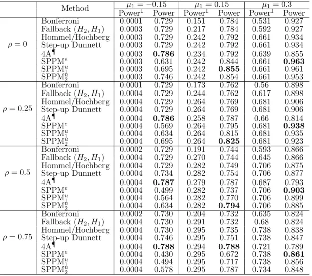
Table 2.3 shows the power under various settings, and the highest power among different testing procedures are in bold. In the two-hypothesis testing framework, the Hochberg and Hommel procedures have the same power due to their testing algorithms. Overall, when the effect sizes are in the same direction, the SPPM procedure outperforms other methods in terms of Power of rejecting at least one hypothesis (Power) and has the comparable power of rejecting both hypotheses (Power1). The SPPM with equal critical values (SPPMe) has higher power than other existing methods when the correlation and/or the discrepancy in the effect sizes are

small; otherwise, the power improvement of SPPMe _{vanishes. The performance of}

the step-up Dunnett procedure is not affected too much by the inconsistency in the effect sizes and has a higher power than the nonparametric procedures when there is a strong correlation between two endpoints as expected. The 4A procedure has obvious advantage when the two effect sizes are different since it aims to accommodate the underpowered hypotheses/endpoints but the prior knowledge is necessary to achieve high power. Those investigated existing approaches are more powerful when one of hypothesis has negative mean, while SPPM procedure provides low power. Although, the SPPM testing procedure does not statistically improve power uniformly, this is actually the desired feature of the proposed procedure from the perspective of clinical trials because, for example, (1) for two endpoints, if one endpoint shows positive effect and the other shows negative effect, the overall benefit of the drug might diminish, the probability of approving such a drug should be small; similarly, (2) in the case of two doses, if one dose has positive effect and the other dose has a negative effect, we should be very caution in approving the drug since patient might not take exact amount of dose as indicated. In this sense, SPPM emphasizes the consistency of the results or the totality of evidence while controlling the FWER as well.

One reason that the SPPMe has lower power in some of the situations is that such a specific defined procedure highlights the consistency of the evidence against both hypotheses, while the inconsistency clearly exists in the case with different effect sizes. Fortunately, Eq. (2.3) allows us to allocate α1 and α2 differently as for SPPMu1

and SPPMu

SPPMu

2 have similar powers when the effect sizes are similar from Table 2.3. The

powers of three SPPM procedures are distinguished from each other when a large difference in the effect sizes exists, and the phenomenon of differential powers is more obvious with the increasing correlation. SPPMe _{performs poorly for the smallµ}

1, but

Table 2.3: Power comparisons for two-hypothesis testing with different correla-tions (µ2 = 0.3, σ = 1).

Method µ1 =−0.15 µ1 = 0.15 µ1 = 0.3

Power1 Power Power1 Power Power1 Power

ρ= 0 Bonferroni 0.0001 0.729 0.151 0.784 0.531 0.927 Fallback (H2, H1) 0.0003 0.729 0.217 0.784 0.592 0.927 Hommel/Hochberg 0.0003 0.729 0.242 0.792 0.661 0.934 Step-up Dunnett 0.0003 0.729 0.242 0.792 0.661 0.934 4A¶ 0.0003 0.786 0.234 0.792 0.639 0.855 SPPMe 0.0003 0.631 0.242 0.844 0.661 0.963 SPPMu₁ 0.0003 0.695 0.242 0.855 0.661 0.961 SPPMu₂ 0.0003 0.746 0.242 0.854 0.661 0.953 ρ= 0.25 Bonferroni 0.0001 0.729 0.173 0.762 0.56 0.898 Fallback (H2, H1) 0.0004 0.729 0.244 0.762 0.617 0.898 Hommel/Hochberg 0.0004 0.729 0.264 0.769 0.681 0.906 Step-up Dunnett 0.0004 0.729 0.264 0.769 0.681 0.906 4A¶ 0.0004 0.786 0.258 0.787 0.66 0.814 SPPMe 0.0004 0.569 0.264 0.795 0.681 0.938 SPPMu₁ 0.0004 0.634 0.264 0.815 0.681 0.935 SPPMu₂ 0.0004 0.695 0.264 0.825 0.681 0.923 ρ= 0.5 Bonferroni 0.0002 0.729 0.191 0.744 0.593 0.866 Fallback (H2, H1) 0.0004 0.729 0.270 0.744 0.645 0.866 Hommel/Hochberg 0.0004 0.729 0.282 0.749 0.706 0.875 Step-up Dunnett 0.0004 0.734 0.282 0.754 0.706 0.877 4A¶ 0.0004 0.787 0.279 0.787 0.687 0.793 SPPMe 0.0004 0.499 0.282 0.737 0.706 0.903 SPPMu₁ 0.0004 0.564 0.282 0.770 0.706 0.899 SPPMu₂ 0.0004 0.634 0.282 0.794 0.706 0.885 ρ= 0.75 Bonferroni 0.0002 0.730 0.204 0.732 0.635 0.824 Fallback (H2, H1) 0.0004 0.730 0.291 0.732 0.68 0.824 Hommel/Hochberg 0.0004 0.730 0.295 0.735 0.738 0.838 Step-up Dunnett 0.0004 0.746 0.295 0.751 0.738 0.847 4A¶ 0.0004 0.788 0.294 0.788 0.721 0.789 SPPMe 0.0004 0.430 0.295 0.672 0.738 0.861 SPPMu₁ 0.0004 0.494 0.295 0.717 0.738 0.856 SPPMu₂ 0.0004 0.578 0.295 0.787 0.734 0.848 Note: N = 90, one-sidedα= 0.025;

The equal weights w1=w2= 0.5 in Bonferroni and Fallback procedures;

¶_{: α}

1= 0.02 for the endpoint withµ2= 0.3 in 4A procedure;

SPPMe: SPPM procedure with the equal critical values (α1=α2);

SPPMu1: SPPM procedure with the unequal critical values (3α1=α2);

SPPMu

In summary, The nonparametric procedures make no assumptions about the joint distribution of test statistics, which results in power loss when the strong correlation exists. The step-up Dunnett improves power by taking advantage of assumptions of the joint distribution and the 4A procedure has dominant strength when the prior information is known with one underpowered hypotheses. The SPPM procedure with the equal critical values improves power compared to other procedures in most situations, although the gain in power is sensitive to the inconsistency in the effect sizes under the alternatives. In practice, when we have little knowledge about the magnitude of effect sizes for the small/moderate correlation, simply applying SPPMe can provide us a powerful testing as well. In addition, if the information about the relative effect sizes is available, the unequal critical values of the SPPM procedure can be utilized to boost power.

2.3.2 Power Comparisons of Three-Hypothesis Testing

As concluded in Section 2.3.1, the Hochberg, Hommel, step-up Dunnett and 4A procedures continues to be compared in the three-hypothesis testing. We also included the parametric graphical approach as the representative of parametric procedures for power comparisons. The equal initial allocation of the significance level (i.e.

α1 = α2 =α3 =α/3) and the same elements as 0.5 for the transition matrix are used,

which is the parametric version of the Bonferroni-Holm procedure and the same as the step-down Dunnett test. For the 4A method,α1 = 0.02 is used again for the hypothesis

overall level α2 using Hochberg’s method. The two versions of SPPM procedure with

equal and unequal critical values are performed to examine the influence of different

α-allocations on the power. The three correlated endpoints are simulated 100,000 replicates with the same pairwise correlation and sample size N as 60. One-sample test is again conducted with known covariance matrix. µ3 is fixed as 0.3 and we varied

µ1 andµ2 to evaluate the performance of the procedures under various correlations

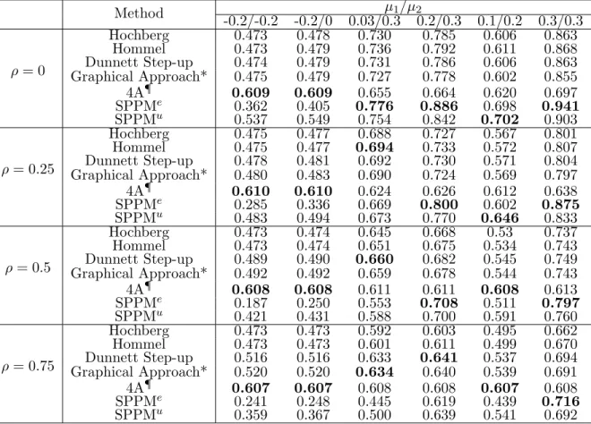
(ρ = 0,0.25,0.5,0.75), which is shown in Table 2.4. The largest values of power are in bold for each scenario. The Hommel procedure is uniformly powerful than the Hochberg procedure with a slight improvement, as also demonstrated before (Dmitrienko et al., 2009). We observe that the SPPM procedure performs the best among all the evaluated methods when the independent hypotheses have the effect sizes in the same direction. When the correlation among the endpoints increases, the advantage of the SPPM procedure with the equal critical values weakens, especially when the effect sizes differ a lot. However, the power loss can be dealt with by using different critical values. Since the step-up Dunnett is the data-driven method, therefore not affected too much by the inconsistency in the effect sizes, and the 4A method targets to improve the power for the underpowered hypotheses with prior knownledge, SPPMu fails to beat those two methods with a large difference in the effect sizes and/or the strong correlation, but SPPM is still comparable to some other methods with properly adjusted critical values. Again, the SPPM testing procedure provides lower power when some hypotheses have null effects, which is preferred sometimes in the clinical trial setting.

Table 2.4: Power comparisons for three-hypothesis testing with differ-ent correlations (µ3 = 0.3, σ= 1). Method µ1/µ2 -0.2/-0.2 -0.2/0 0.03/0.3 0.2/0.3 0.1/0.2 0.3/0.3 ρ= 0 Hochberg 0.473 0.478 0.730 0.785 0.606 0.863 Hommel 0.473 0.479 0.736 0.792 0.611 0.868 Dunnett Step-up 0.474 0.479 0.731 0.786 0.606 0.863 Graphical Approach* 0.475 0.479 0.727 0.778 0.602 0.855 4A¶ 0.609 0.609 0.655 0.664 0.620 0.697 SPPMe 0.362 0.405 0.776 0.886 0.698 0.941 SPPMu 0.537 0.549 0.754 0.842 0.702 0.903 ρ= 0.25 Hochberg 0.475 0.477 0.688 0.727 0.567 0.801 Hommel 0.475 0.477 0.694 0.733 0.572 0.807 Dunnett Step-up 0.478 0.481 0.692 0.730 0.571 0.804 Graphical Approach* 0.480 0.483 0.690 0.724 0.569 0.797 4A¶ 0.610 0.610 0.624 0.626 0.612 0.638 SPPMe 0.285 0.336 0.669 0.800 0.602 0.875 SPPMu 0.483 0.494 0.673 0.770 0.646 0.833 ρ= 0.5 Hochberg 0.473 0.474 0.645 0.668 0.53 0.737 Hommel 0.473 0.474 0.651 0.675 0.534 0.743 Dunnett Step-up 0.489 0.490 0.660 0.682 0.545 0.749 Graphical Approach* 0.492 0.492 0.659 0.678 0.544 0.743 4A¶ 0.608 0.608 0.611 0.611 0.608 0.613 SPPMe 0.187 0.250 0.553 0.708 0.511 0.797 SPPMu 0.421 0.431 0.588 0.700 0.591 0.760 ρ= 0.75 Hochberg 0.473 0.473 0.592 0.603 0.495 0.662 Hommel 0.473 0.473 0.601 0.611 0.499 0.670 Dunnett Step-up 0.516 0.516 0.633 0.641 0.537 0.694 Graphical Approach* 0.520 0.520 0.634 0.640 0.539 0.691 4A¶ 0.607 0.607 0.608 0.608 0.607 0.608 SPPMe 0.241 0.248 0.445 0.619 0.439 0.716 SPPMu 0.359 0.367 0.500 0.639 0.541 0.692 Note: N = 60, one-sidedα= 0.025;

*: Equal initial allocation ofαand the elements as 0.5 for the transition matrix are used;

¶_{: α}

1 = 0.02 for the endpoint with µ3= 0.3 and the other two endpoints were assessed at an

adaptive overall level using Hochberg’s method in 4A method; SPPMe_{: SPPM procedure with the equal critical values (α}

1=α2=α3);

SPPMu_{: SPPM procedure with the unequal critical values (10α}

2.3.3 The FWER with Unknown Covariance Matrix

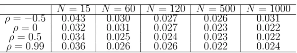
The SPPM testing procedure takes into account the correlation among test statistics to control the FWER. With the known correlation coefficient at the design stage, the procedure could perform accurately. Correlations can also be estimated with the sample data, however, the use of sample correlations could potentially inflate the error rate. Additionally, it is unlikely to know the true variance sometimes in practice, and the estimated variance could potentially inflate the type I error rate. To explore the effect of using the estimated covariance matrix from the sample on the FWER, the case of the two endpoints in one-sample test is studied through simulations. The observed

p-value is calculated using Z-statistic with the estimated variance, the correlation is estimated from the sample data, denoted as ˆρ, and the equal critical values are calculated from Eq. (2.4) with ρ replaced by ˆρ. Based on 100,000 simulations, the FWER under the global null (Table 2.5) with the estimated variance and correlation is controlled when the sample size is larger than 500 for a typical phase III trial, for which FWER is critical. For a smaller sample size, around 60-100, an error rate inflation is observed while is within the acceptant limit. However, since this is a typical sample size for a phase II trial, for which FWER is not as critical as phase III trial, such a small inflation should be acceptable. The FWER under other two configurations of null hypothesis is shown in Appendix (Table F.1) and it is also well-controlled for large sample size. Therefore, we recommend to apply the SPPM testing procedure in the phase II/III trials when there is no information about the variance and correlation