Friedrich Leisch
Neighborhood Graphs, Stripes and Shadow Plots
for Cluster Visualization
Technical Report Number 061, 2009
Department of Statistics
University of Munich
Neighborhood Graphs, Stripes and Shadow Plots
for Cluster Visualization
Friedrich Leisch
Institut f¨ur Statistik, Ludwig-Maximilians-Universit¨at M¨unchen
Ludwigstrasse 33, 80539 Munich, Germany
This is a preprint of an article that has been accepted for publication in
Statistics and Computing
.
Please use the journal version for citation.
Abstract
Centroid-based partitioning cluster analysis is a popular method for segmenting data into more homogeneous subgroups. Visualization can help tremendously to understand the positions of these subgroups relative to each other in higher dimensional spaces and to assess the quality of partitions. In this paper we present several im-provements on existing cluster displays using neighborhood graphs with edge weights based on cluster separation and convex hulls of inner and outer cluster regions. A new display called shadow-stars can be used to diagnose pairwise cluster separation with respect to the distribu-tion of the original data. Artificial data and two case studies with real data are used to demon-strate the techniques.
Key Words: cluster analysis, partition, cen-troid, convex hull, R.
1 Introduction
The goal of cluster analysis is to either find ho-mogeneous subgroups of the data, which in the best of all cases in turn are as different as pos-sible from each other; or to impose an artificial grouping on the data. In any case we want to in-crease our understanding of the data by a divide & conquer approach which partitions a poten-tially complex and large data set into segments (i.e., clusters) that are easier to understand or handle.
Data visualization can help a lot to under-stand multivariate data structures, hence it is no surprise that cluster analysis and data visualiza-tion often go hand in hand. Standard textbooks on cluster analysis like Gordon (1999) or Everitt et al. (2001) are full of figures, see also Leisch (2008) for a recent survey on cluster visualiza-tion. Results from partitioning cluster analysis can be visualized by projecting the data into 2-dimensional space (e.g., CLUSPLOT, Pison et al., 1999). Cluster membership in the pro-jection is usually represented by different colors and glyphs, or by dividing clusters onto several panels of a Trellis display (Becker et al., 1996). In addition, silhouette plots (Rousseeuw, 1987) are a popular tool for diagnosing the quality of a partition. Parts of the popularity of self-organizing feature maps (Kohonen, 1989) with practitioners in various fields can be explained by the fact that the results can be “easily” visu-alized.
In this paper we introduce several improve-ments and modifications of existing cluster vi-sualization techniques, and propose a new diag-nostic display we call shadow-stars. The exact choice of distance measure or partitioning clus-ter algorithm is not important. The only condi-tion is that it is centroid-based, i.e., clusters are represented by prototypes and data points are assigned to the cluster corresponding to the clos-est prototype. Many popular clustering algo-rithms likek-means (MacQueen, 1967; Hartigan and Wong, 1979), partitioning around medoids (PAM, Kaufman and Rousseeuw, 1990) or neu-ral gas (Martinetz and Schulten, 1994) fall into
this category.
All methods introduced in this paper have been implemented in the statistical computing environment R (R Development Core Team, 2008) and will be released as part of the R ex-tension package flexclust (Leisch, 2006) on the Comprehensive R Archive Network (CRAN, http://cran.R-project.org) under the terms of the GPL.
The rest of this paper is organized as follows: Section 2 give a reminder of centroid-based clus-ter analysis, neighborhood graphs and shadow values, which form the basis for the following sections. Sections 3– 6 introduce several new ways to visualize and diagnose cluster solutions. Stripes plots directly show the distance of data points to cluster centroids, while shadow plots relate the distance to the closest and second-closest centroid. Shadow stars can be used to assess which cluster’s are close to each other. Convex cluster hulls allow to shade cluster re-gions for non-elliptical cluster shapes. These new graphical technices are demonstrated on data from automobile marketing in Section 7 and data from German parliamentary elections in Section 8.
2 Neighborhood
Graphs
and Shadow Values
Assume we are given a data set XN =
{x1, . . . ,xN}, xn ∈ Rp and a set of centroids
CK = {c1, . . . ,cK}, ck ∈ Rp which is the
re-sult of a centroid-based cluster analysis likeK -means. Let d(x,y) denote a distance measure onRp(xandy∈Rp), let
c(x) = argmin
c∈CK
d(x,c) denote the centroid closest tox, and
Ak ={xn∈XN|c(xn) =ck}
be the set of all points where ck is the clos-est centroid. For simplicity of notation we as-sume that all clusters are non-empty, such that
|Ak| > 0,∀k = 1, . . . , K (our software
imple-mentation automatically removes empty clus-ters accordingly). Most cluster algorithms will try to find a set of centroidsCKfor fixedKsuch
that the average distance D(XN, CK) =N1 N X n=1 d(xn, c(xn))→minC K,
of each point to the closest centroid is mini-mal. However, for the following it is not im-portant whether such an optimum has actually been reached.
Leisch (2006) introduces aneighborhood graph
of the centroids where each centroid forms a node and two nodes are connected by an edge if there exists at least one data point for which those two are closest and second closest, see also Martinetz and Schulten (1994). Let
˜
c(x) = argmin
c∈CK\{c(x)}d(x,c)
denote the second-closest centroid tox, further let
Aij={xn∈XN|c(xn) =ci,c(˜xn) =cj}
be the set of all points where ci is the closest centroid andcjis second-closest. Now we define for each observation x its shadow value s(x) as
s(x) = d(x, c(2d(x)) +x, c(d(x,x))c(˜x))
The name “shadow” was chosen because the shadow of an object is similar to its silhouette, and the shadow plots constructed below are sim-ilar both in spirit and interpretation to the well known silhouette plots (Rousseeuw, 1987). If s(x) is close to 0, then the point is close to its cluster centroid. If s(x) is close to 1, it is al-most equidistant to the two centroids. Thus, a cluster that is well separated from all other clus-ters should have many points with small shadow values.
Another memory aid is that the shadow value of a point gives the relative location of the shadow the point casts upon the line connect-ing c(x) and ˜c(x). A cluster with large shadow values “casts a large shadow on its neighbouring clusters”, and hence is close to them.
The average shadow value of all points where clusteriis closest andjis second-closest can be used as a simple measure of cluster similarity:
sij=|Ai|−1
X
x∈Aij
s(x)
The denominator |Ai|rather than |Aij|is used
such that a small setAijconsisting only of badly
clustered points with large shadow values does not induce large cluster similarity. If sij > 0,
then at least one data point in segmentihascj
are neighbours. Ifsij is close to|Aij|/|Ai|, then
those points that are “between” segmentsiand j are almost equidistant to the two centroids. The graph with nodes ck and edge weights sij
is a directed graph, to simplify matters we use the corresponding undirected graph with aver-age values ofsij andsjias edge weights for the
moment.
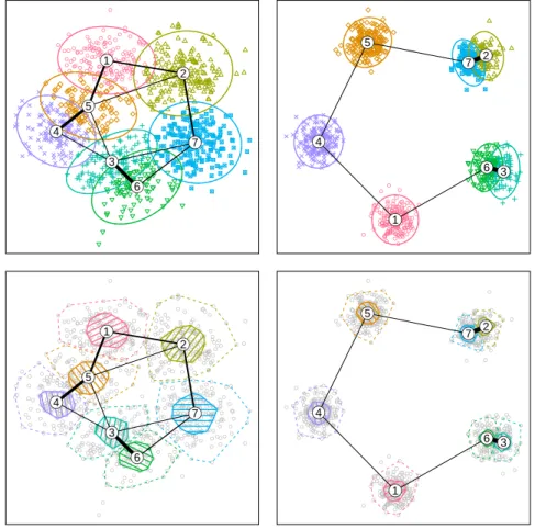
Figure 1 shows neighborhood graphs for two data sets with 5 Gaussian clusters each. The graphs in panels above each other are identical, the different cluster hulls will be explained in Section 6. The centers of the original 5 clusters are identical in both data sets, only the variance changes. Both data sets have been clustered us-ingK-means with 7 centers. The “wrong” num-ber of clusters was intentional to show the effect on the graph and get overlapping clusters.
Both graphs show the ring-like structure of the data, the thickness of the lines is propor-tional to the edge weights and clearly shows how well the corresponding clusters are separated. Triangular structures like in the left panel corre-spond to regions with almost uniform data den-sity that are split into several clusters. Centroid pairs connected by one thick line and only thin lines to the rest of the graph like 2/7 and 3/6 in the right panel correspond to a well-separated data cluster that has wrongly been split into two clusters.
3 Stripes Plots
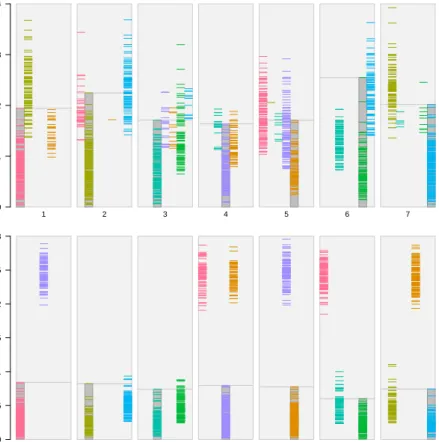
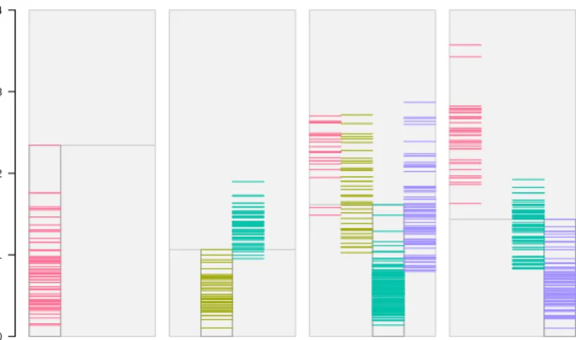
A simple, yet very effective plot for visualiz-ing the distance of each point from its closest and second-closest cluster centroids is a stripes plot as shown in Figure 2. For each cluster k= 1, . . . , Kwe have a rectangular area, which we vertically divide into K smaller rectangles. First we draw a horizontal line segment hat height (xn, c(xn)) for each observationxn∈Ak.
In addition, we plot a horizontal line segment for each observation xn ∈ Ajk, j = 1, . . . , K,
æ6=kat heightd(xn,ck). These are the points which have cluster kas their second-best. The horizontal position within the rectangular area and the color (please use the online version of this article for colored figures) always mark the clusterc(xn) of the observation.
E.g., have a look at cluster 1 in the top panel. The leftmost stripe corresponds to points that have been assigned to cluster 1. It is marked by a slightly darker background and a box around
the stripe. Points in clusters 2 and 5 have clus-ter 1 as second-best centroid. These observa-tions form the other two stripes within the rect-angular area for cluster 1. Points in cluster 2 are farther away from cluster 1, while many points in cluster 5 have a similar distance to centroid 1 as points which have actually been assigned to cluster 1.
The overall impression of the top panel in Fig-ure 2 is that no cluster is well separated from all others. We can also infer which one of the other clusters is close to it. The picture is different for the bottom panel: clusters 1, 4, and 5 are well separated from the rest (the lowest block of stripes is far away from the rest), while clusters 2/7 and 3/6 are close to each other, respectively. Of course all this information is easier to see in Figure 1, however the stripes plot is dimension-independent and works well even for high-dimensional data where projections to 2d may fail. The implementation of the stripes plot in our software is very flexible. The user can zoom into the bars to see only distances from the closest cluster centroid of each point, or only see distances to closest and second-closest centroid. It is also possible to choose a categorical back-ground variable for the color-coding. This gives a quick overview of how the classes in the back-ground variable are distributed over the clusters, and if they are close to the centroid or far away (see Section 8 below).
4 Shadow Plots
Another way to visualize the separation are clus-ter silhouettes (Rousseeuw, 1987). The silhou-ette value ofx
sil(x) = max(a(b(x)−x), b(a(xx)))
is defined as the scaled difference between the average dissimilaritya(x) ofxto all points in its own cluster to the smallest average dissimilarity b(x) to the points of a different cluster. For shadow values we get
1−s(x) = 1−d(x, c(2d(x)) +x, c(d(xx)),˜c(x))
= d(d(x, c(x,˜c(xx)) +))−d(d(xx, c(,c(˜xx)))) and a plot of 1−s(x) can be used to approximate silhouettes. The main difference between silhou-ette values and shadow values is that we replace
● ● ● ● ● ● ● ● ● ● ● ● ● ● ● ● ● ● ● ● ● ● ● ● ● ● ● ● ● ● ● ● ● ● ● ● ● ● ● ● ● ● ● ● ● ● ● ● ● ● ● ● ● ● ● ● ● ● ● ● ● ● ● ● ● ● ● ● ● ● ● ● ● ● ● ● ● ● ● ● ● ● ● ●● ● ●● ● ● ● ● ● ● ● ● ● ● ● ● ● ● ● ● ● ● ● ● ● ● ● ● ● ● ● ● ● ● ● ● ● ● ● ● ● ● ● ● ● ● ● ● ● ● ● ● ● ● ● ● ● ● ● ● ● ● ●● ● ● ● ● ● ● ● ● ● ● ● ● ● ● ● ● ● ● ● ● ● 1 2 3 4 5 6 7 ● ●● ● ● ● ● ● ● ● ● ● ● ● ● ● ● ● ● ● ● ● ● ● ● ● ● ● ● ● ● ● ● ● ● ● ● ● ● ● ● ● ● ● ● ● ● ● ● ●●● ● ● ● ● ● ● ● ● ● ● ● ● ● ● ● ● ● ● ● ● ● ● ● ● ● ● ● ● ● ● ● ● ● ● ● ● ● ● ● ● ● ● ● ● ● ● ● ● ● ● ● ● ● ● ● ● ● ● ● ● ● ● ● ● ● ● ● ● ● ● ● ●● ● ● ● ● ● ● ● ● ● ● ● ● ● ● ● ● ● ● ● ● ● ●● ● ● ● ● ● ● ● ● ● ● ● ● ● ● ● ● ● ● ● ● ● ● ● ● ● ● ● ● ● ● ● ● ● ● ● ● ● ●● ● ● ● ●● ● ● ● ● ● ● ● ● ● ● ● ● 1 2 3 4 5 6 7 ● ● ● ● ● ● ● ● ● ● ● ● ● ● ● ● ● ● ● ● ● ● ● ● ● ● ● ● ● ● ● ● ● ● ● ● ● ● ● ● ● ● ● ● ● ● ● ● ● ● ● ● ● ● ● ● ● ● ● ● ● ● ● ● ● ● ● ● ● ● ● ● ● ● ● ● ● ● ● ● ● ● ● ● ● ● ● ● ● ● ● ● ● ● ● ● ● ● ● ● ● ● ● ● ● ● ● ● ● ● ● ● ● ● ● ● ● ● ● ● ● ● ● ● ● ● ● ● ● ● ● ● ● ● ● ● ● ● ● ● ● ● ● ● ● ● ● ● ● ● ● ● ● ● ● ● ● ● ● ● ● ● ● ● ● ● ● ● ● ● ● ● ● ● ● ● ● ● ● ● ● ● ● ● ● ● ● ● ● ● ● ● ● ● ● ● ● ● ● ● ● ● ● ● ● ● ● ● ● ● ● ● ● ● ● ● ● ● ● ● ● ● ● ● ● ● ● ● ● ● ● ● ● ● ● ● ● ● ● ● ● ● ● ● ● ● ● ● ● ● ● ● ● ● ● ● ● ● ● ● ● ● ● ● ● ● ● ● ● ● ● ● ● ● ● ● ● ● ● ● ● ● ● ● ● ● ● ● ● ● ● ● ● ● ● ● ● ● ● ● ● ● ● ● ● ● ● ● ● ● ● ● ● ● ● ● ● ● ● ● ● ● ● ● ● ● ● ● ● ● ● ● ● ● ● ● ● ● ● ● ● ● ● ● ● ● ● ● ● ● ● ● ● ● ● ● ● ● ● ● ● ● ● ● ● ● ● ● ● ● ● ● ● ● ● ● ● ● ● ● ● ● ● ● ● ● ● ● ● ● ● ● ● ● ● ● ● ● ● ● ● ● ● ● ● ● ● ● ● ● ● ● ● ● ● ● ● ● ● ● ● ● ● ● ● ● ● ● ● ● ● ● ● ● ● ● ● ● ● ● ● ● ● ● ● ● ● ● ● ● ● ● ● ● ● ● ● ● ● ● ● ● ● ● ● ● ● ● ● ● ● ● ● ● ● ● ● ● ● ● ● ● ● ● ● ● ● ● ● ● ● ● ● ● ● ● ● ● ● ● ● ● ● ● ● ● ● ● ● ● ● ● ● ● ● ● ● ● ● ● ● ● ● ● ● ● ● ● ● ● ● ● ● ● ● ● ● ● ● ● ● ● ● ● ● ●● ● ● ● ● ● ● ● ● ● ● ● ● ● ● ● ● ● ● ● ● ● ● ● ● ● ● ● ● ● ● ● ● ● ● ● ● ● ● ● ● ● ● ●● ● ● ● ● ● ● ● ● ● ● ● ● ● ● ● ● ● ● ● ● ● ● ● ● ● ● ● ● ● ● ● ● ● ● ● ● ● ● ● ● ● ● ● ● ● ● ● ● ● ● ● ● ● ● ● ● ● ● ● ● ● ● ● ● ● ● ● ● ● ● ● ● ● ● ● ● ● ● ● ● ● ● ● ● ● ● ● ● ● ● ● ● ● ● ● ● ● ● ● ● ● ● ● ● ● ● ● ● ● ● ● ● ● ● ● ● ● ● ● ● ● ● ● ● ● ● ● ● ● ● ● ● ● ● ● ● ● ● ● ● ● ● ● ● ● ● ● ● ● ● ● ● ● ● ● ● ● ● ● ● ● ● ● ● ● ● ● ● ● ● ● ● ● ● ● ● ● ● ● ● ● ● ● ● ● ● ● ● ● ● ● ● ● ● ● ● ● ● ● ● ● ● ● ● ● ● ● ● ● ● ● ● ● ● ● ● ● ● ● ● ● ● ● ● ● ● ● ● ● ● ● ● ● ● ● ● ● ● ● ● ● ● ● ● ● ● ● ● ● ● ● ● ● ● ● ● ● ● ● ● ● ● ● ● ● ● ● ● ● ● ● ● ● ● ● ● ● ● ● ● ● ● ● ● ● ● ● ● ● ● ● ● ● ● ● ● ● ● ● ● ● ● ● ● ● ● ● ● ● ● ● ● ● ● ● ● ● ● ● ● ● ● ● ● ● ● ● ● ● ● ● ● ● ● ● ● ● ● ● ● ● ● ● ● ● ● ● ● ● ● ● ● ● ● ● ● ● ● ● ● ● ● ● ● ● ● ● ● ● ● ● ● ● ● ● ● ● ● ● ● ● ● ● ● ● ● ● ● ● ● ● ● ● ● ● ● ● ● ● ● ● ● ● ● ● ● ● ● ● ● ● ● ● ● ● ● 1 2 3 4 5 6 7 ● ● ● ● ● ● ● ● ● ● ●● ● ● ● ● ● ● ● ● ● ● ● ● ● ● ● ● ● ● ● ● ● ● ● ● ● ● ● ● ● ● ● ● ● ● ● ● ● ● ● ● ● ● ● ● ● ● ● ● ● ● ● ● ● ● ● ● ● ● ● ● ● ● ● ● ● ● ● ● ● ● ● ● ● ● ● ● ● ● ● ● ● ● ● ● ● ● ● ● ● ● ● ● ● ● ● ● ● ● ● ● ● ● ● ● ● ● ● ● ● ● ● ● ● ● ● ● ● ● ● ● ● ● ● ● ● ● ● ● ● ● ● ● ● ● ● ● ● ● ● ● ● ● ● ● ● ● ● ● ● ● ● ● ● ● ● ● ● ● ● ● ● ● ● ● ● ● ● ● ● ● ● ● ● ● ● ● ● ● ● ● ● ● ● ● ● ● ● ● ● ● ● ● ● ● ● ● ● ● ● ● ● ● ● ● ● ● ● ● ● ● ● ● ● ● ● ● ● ● ● ● ● ● ● ● ● ● ● ● ● ● ● ● ● ● ● ● ● ● ● ● ● ● ● ● ● ● ● ● ● ● ● ● ● ● ● ● ● ● ● ● ● ● ● ● ● ● ● ● ● ● ● ● ● ● ● ● ● ● ● ● ● ● ● ● ● ● ● ● ● ● ● ● ● ● ● ● ● ● ● ● ● ● ● ● ● ● ● ● ● ● ● ● ● ● ● ● ● ● ● ● ● ● ● ● ● ● ● ● ● ● ● ● ● ● ● ● ● ● ● ● ● ● ● ● ● ● ● ● ● ● ● ● ● ● ● ● ● ● ● ● ● ● ● ● ● ● ● ● ● ● ● ● ● ● ● ● ● ● ● ● ● ● ● ● ● ● ● ● ● ● ● ● ● ● ● ● ● ● ● ● ● ● ● ● ● ● ● ● ● ● ● ● ● ● ● ● ● ● ● ● ● ● ● ● ● ● ● ● ● ● ● ● ● ● ● ● ● ● ● ● ● ● ● ● ● ● ● ● ● ● ● ● ● ● ● ● ● ● ●● ● ● ● ● ● ● ● ● ● ● ● ● ● ● ● ● ● ● ● ● ● ● ● ● ● ● ● ● ● ● ● ● ● ● ● ● ● ● ● ● ● ● ● ● ● ● ● ● ● ● ● ● ● ● ● ● ● ● ● ● ● ● ● ● ● ● ● ● ● ● ● ● ● ● ● ● ● ● ● ● ● ● ● ● ● ● ● ● ● ● ● ● ● ● ● ● ● ● ● ● ● ● ● ● ● ● ● ● ● ● ● ● ● ● ● ● ● ● ● ● ● ● ● ● ● ● ● ● ● ● ● ● ● ● ● ● ● ● ● ● ● ● ● ● ● ● ● ● ● ● ● ● ● ● ● ● ● ● ● ● ● ● ● ● ● ● ● ● ● ● ● ● ● ● ● ● ● ● ● ● ● ● ● ● ● ● ● ● ● ● ● ● ● ● ● ● ● ● ● ● ● ● ● ● ● ● ● ● ● ● ● ● ● ● ● ● ● ● ● ● ● ● ● ● ● ● ● ● ● ● ● ● ● ● ● ● ● ● ● ● ● ● ● ● ● ● ● ● ● ● ● ● ● ● ● ● ● ● ● ● ● ● ● ● ● ● ● ● ● ● ● ● ● ● ● ● ● ● ● ● ● ● ● ● ● ● ● ● ●● ● ● ● ● ● ● ● ● ● ● ● ● ● ● ● ● ● ● ● ● ● ● ● ● ● ● ● ● ● ● ● ● ● ● ● ● ● ● ● ● ● ● ● ● ● ● ● ● ● ● ● ● ● ● ● ● ● ● ● ● ● ● ● ● ● ● ● ● ● ● ● ● ● ● ● ● ● ● ● ● ● ● ● ● ● ● ● ● ● ● ● ● ● ● ● ● ● ● ● ● ● ● ● ● ● ● ● ● ● ● ● ● ● ● ● ● ● ● ● ● ● ● ● ● ● ● ● ● ● ● ● ● ● ● ● ● ● ● ● ● ● ● ● ● ● ● ● ● ● ● ● ● ● ● ● ● ● ● ● ● ● ● ● ● ●● ● ● ● ● ● ● ● ● ● ● ● ● ● ● ● ● ● ● ● ● ● ● ● ● ● ● ● ● ● ● ● ● ● ● ● ● ● ● ● ● ● ● ● ● ● ● ● ● ● ● ● ● ● ● ● ● ● ● ● ● ● ● ● ● ● ● ● ● ● ● ● ● x2$x[,2] ● ● ● ● ● ● ● 1 2 3 4 5 6 7
Figure 1: The neighborhood graphs for 7-cluster partitions of 5 Gaussians with poor (left top and bottom) and good (right top and bottom) separation.
0 1 2 3 4 1 2 3 4 5 6 7 0 0.5 1 1.5 2 2.5 3 1 2 3 4 5 6 7
Figure 2: Stripes plots for the Gaussian data with poor (top) and good (bottom) separation. The seven clusters are on the x-axis, distance from centroid is on the y-axis.
average dissimilarities to points in a cluster by dissimilarities to point averages (=centroids). One advantage of shadow values is that they need O(NK) operations while silhouettes need
O(N2), and typically we haveK << N.
Pack-age flexclust has implementations for both traditional silhouttes, as well as our newshadow
plots which directly visualize the shadow values
s(x) (rather than 1−s(x)).
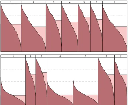
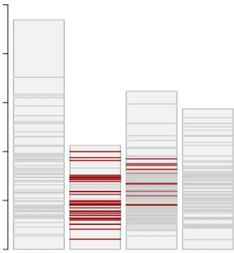
Figure 3 showsshadow plots for both parti-tions. The shadow valuess(x) in each cluster are sorted from high to low and plotted from left to right. To decrease memory consumption the ac-tual values are interpolated for larger data sets. The width of the vertical stripe of each cluster is proportional to the size of the cluster. Clus-ters that are well separated should have many points with small shadow values s(x), and the filled area below the curve should be small. The light rectangle behind the polygon marks the average shadow value of the cluster, hence the area of the rectangle in light color is the same as the area under the shadow line filled with dark color. This visual aid helps a lot to quickly com-pare the areas under the polygon.
The upper panel of Figure 3 shows the shadow plot for the Gaussian data with poor separa-tion. Points are almost uniformly spread be-tween the closest and second centroid, so the curves in all stripes go almost linearly from 1 to 0. The lower panel has 4 clusters with poor sepa-ration (2,3,6,7) looking similar to the shadows in the upper panel. The 3 clusters with good sep-aration (1,4,5) clearly have a different shadow. The curve starts around 0.5 rather than one, the filled area consequently is much smaller.
5 Shadow-Stars
The main reason for our definition of shadow values is that they use the centroids as anchor points and have a geometric interpretation with respect to them. The distribution of the shadow values of all points in Aij and Ajigives an
im-pression how connected or separated clusters i andj are. Points withs(x)≈0 are close to the centroid, while points withs(x)≈1 are equidis-tant to c(x) and ˜c(x). This can be visualized in a new display, the shadow-stars: The cen-troids again are used as nodes in a graph, which are connected by stripe plots of shadow values. If Aij is not empty, then a (virtual) line
seg-ment fromci tocj is drawn. The width of the
line segments is proportional to the size ofAij,
such that larger groups of data can be identified more easily. On the half segment closer to ci
the shadow values inAij are drawn as line
seg-ments similar to the stripes plot. On the other half of the line segment the same is done with the shadow values of the points in Aji. If
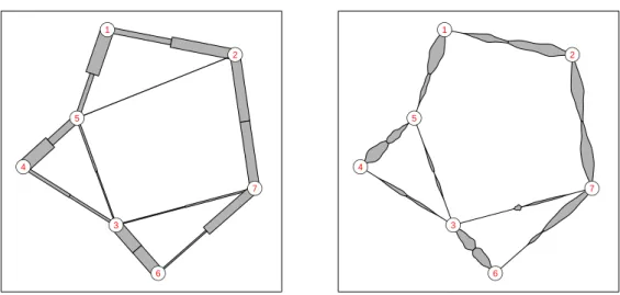
clus-ter i is well separated from clusterj, then the shadow values will be small and the stripes will be concentrated close to the centroid. On the other hand, if the two clusters are not well sep-arated, then the stripes of shadow values will either have an almost uniform distribution or be concentrated close to the middle of the edge. Figure 4 shows shadow-stars for the Gaussian data. The clusters in the left panel are not well separated, the shadow values are distributed over the line segments connecting neighboring clusters. For the well separated clusters in the right panel the shadow values concentrate their mass close to the centroids. It can still be seen from the plot which cluster is next to which other cluster, but it is also obvious that they are far away from each other in terms of cluster separation.
Again, the software implementation is very flexible, and the user can specify arbitrary func-tions which are used to visualize the shadow values on each half-edge of the graph. If we use only the average shadow value as thickness of the edge, we get an asymmetric graph we call a shadow skeleton. If we use violin plots (Hintze and Nelson, 1998) for the distribution of the shadow values, we getshadow violins, see Figure 5.
6 Convex Cluster Hulls
When clustering non-Gaussian data and/or us-ing distances other than Euclidean distance, spanning ellipses or confidence ellipses like in the CLUSPLOT by Pison et al. (1999) can be a misleading representation of cluster re-gions, because clusters may have arbitrary con-vex shapes, where the term concon-vex is with re-spect to the distance measure used. If clus-ters are projected into 2-dimensional space, then bagplots (Rousseeuw et al., 1999) can be used as a nonparametric alternative to ellipses. The main challenge in constructing the equivalent of a box & whisker plot for 2 dimensions is that
R2has no total ordering. Bagplots solve this by
1 2 3 4 5 6 7
1 2 3 4 5 6 7
Figure 3: Shadow plots for the Gaussian data with poor (top) and good (bottom) separation.
●
●
●
●
●
●
●
1 2 3 4 5 6 7●
●
●
●
●
●
●
1 2 3 4 5 6 7●
●
●
●
●
●
●
1 2 3 4 5 6 7●
●
●
●
●
●
●
1 2 3 4 5 6 7Figure 5: Shadow skeleton (left) and shadow violins (right) for the Gaussian data with poor separation.
that the definition of the “inner 50%” of data becomes feasible.
For data partitioned using a centroid-based cluster algorithm there is a natural total order-ing for each point in a cluster (Leisch, 2008): The distance d(x, c(x)) of the point to its re-spective cluster centroid. Let
mk= median{d(xn,ck)|xn∈Ak}
be the median distance of all points in cluster k to ck. We visualize theinner area a cluster occupies by the convex hull of all data points where d(xn,ck) ≤ mk, this corresponds to the
box in a boxplot. After some experimentation we chose to define the outer area of a cluster as the convex hull of all data points that are no more than 2.5mkaway fromck, this corresponds
to the whiskers in a boxplot. Points outside this area are considered as outliers.
Figure 1 compares the convex hulls of the clusters (bottom row) with 95% confidence el-lipses (top row). As the data are a mixture of bivariate Gaussians, confidence ellipses are a “valid” visualization of the clusters, but only if the true number of clusters is known and found. As we have deliberately used a wrong number of clusters, several clusters have a non-elliptical shape, especially those splitting an underlying true cluster into two. To make the inner area more visible we use diagonal shading lines. As a new feature we use an angle of kπ/K for the lines of cluster k, such that overlapping clus-ters can be distinguished more easily, especially when no colors are available. Obviously, this
could be improved upon by selecting orthogonal directions for clusters which are close to each other.
7 Example 1: Automobile
Customer Survey
As first example demonstrating the proposed vi-sualization techniques we use data from an au-tomobile customer survey from 1983. A Ger-man car Ger-manufacturer sent a questionnaire to 2000 customers who had bought a new car ap-proximately 3 months earlier, 793 of which re-turned a form without missing values. The full data set with 46 variables can be downloaded from the Statistics Department of the University of Munich athttp://www.statistik.lmu.de/ service/datenarchiv/. In the following we consider 21 binary variables on the characteris-tics of the vehicle and manufacturer: clearness, efficiency, driving properties, service, interior, quality, technology, model stability, comfort, re-liability, handling, reputation of manufacturer, concept, character, power, resell value, styling, safety, sport, fuel consumption, and space. Each customer was asked to mark the most important characteristics that led him to buy one of the companies cars.
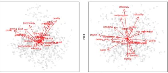
Figure 6 shows biplots of a principal com-ponent (PC) analysis of the data. The left panel gives a scatterplot of all data points projected on PC1 and PC2. There are 2 main directions in the plot, pointing
● ● ● ● ● ● ● ● ● ● ● ● ● ● ● ● ● ● ● ● ● ● ● ● ● ● ● ● ● ● ● ● ● ● ● ● ● ● ● ● ● ● ● ● ● ● ● ● ● ● ● ● ● ● ● ● ● ● ● ● ● ● ● ● ● ● ● ● ● ● ● ● ● ● ● ● ● ● ● ● ● ● ● ● ● ● ● ● ● ● ● ● ● ● ● ● ● ● ● ● ● ● ● ● ● ● ● ● ● ● ● ● ● ● ● ● ● ● ● ● ● ● ● ● ● ● ● ● ● ● ● ● ● ● ● ● ● ● ● ● ● ● ● ● ● ● ● ● ● ● ● ● ● ● ● ● ● ● ● ● ● ● ● ● ● ● ● ● ● ● ● ● ● ●● ● ● ● ● ● ● ● ● ● ● ● ● ● ● ● ● ● ● ● ● ● ● ● ● ● ● ● ● ● ● ● ● ● ● ● ● ● ● ● ● ● ● ● ● ● ● ● ● ● ● ● ● ● ● ● ● ● ● ● ● ● ● ● ● ● ● ● ● ● ● ● ● ● ● ● ● ● ● ● ● ● ● ● ● ● ● ● ● ● ● ● ● ● ● ● ● ● ● ● ● ● ● ● ● ● ● ● ● ● ● ● ● ● ● ● ● ● ● ● ● ● ● ● ● ● ● ● ● ● ● ● ● ● ● ● ● ● ● ● ● ● ● ● ● ● ● ● ● ● ● ● ● ● ● ● ● ● ● ● ● ● ● ● ● ● ● ● ● ● ● ● ● ● ● ● ● ● ● ● ● ● ● ● ● ● ● ● ● ● ● ● ● ● ● ● ● ● ● ● ● ● ●● ● ● ● ● ● ● ● ● ● ● ● ● ● ● ● ● ● ● ● ● ● ● ● ● ● ● ● ● ● ● ● ● ● ● ● ● ● ● ● ● ● ● ● ● ● ● ● ● ● ● ● ● ● ● ● ● ● ● ● ● ● ● ● ● ● ● ● ● ● ● ● ● ● ● ● ● ● ● ● ● ● ● ● ● ● ● ● ● ● ● ● ● ● ● ● ● ● ● ● ● ● ● ● ● ● ● ● ● ● ● ● ● ● ● ● ● ● ● ● ● ● ● ● ● ● ● ● ● ● ● ● ● ● ● ● ● ● ● ● ● ● ● ● ● ● ● ● ● ● ● ● ● ● ● ● ● ● ● ● ● ● ● ● ● ● ● ● ● ● ● ● ● ● ● ● ● ● ● ● ● ● ● ● ● ● ● ● ● ● ● ● ● ● ● ● ● ● ● ● ● ● ● ● ● ● ● ● ● ● ● ● ● ● ● ● ● ● ● ● ● ● ● ● ● ● ● ● ● ● ● ● ● ● ● ● ● ● ● ● ● ● ● ● ● ● ● ● ● ● ● ● ● ● ● ● ● ● ● ● ● ● ● ● ● ● ● ● ● ● ● ● ● ● ● ● ● ● ● ● ● ● ● ● ● ● ● ● ● ● ● ● ● ● ● ● ● ● ● ● ● ● ● ● ● ● ● ● ● ● ● ● ● ● ● ● ● ● ● ● ● ● ● ● ● ● ● ● ● ● ● ● ● ● ● ● ● ● ● ● ● ● ● ● ● ● ● ● ● ● ● ● ● ● ● ● ● ● ● ● ● ● ● ● ● ● ● ● ● ● ● ● ● ● ● ● ● ● ● ● ● ● ● ● ● ● ● ● ● ● ● ● ● ● ● ● ● ● ● ● ● ● ● ● ● ● ● ● ● ● ● ● ● ● ● ●
Principal Components 1 & 2
PC 1 PC 2 clearness efficiency driving_prop service interior quality technology model_stab comfortreliability handling reputation concept character power resell styling safety sport consumption space ● ● ● ● ● ● ● ● ● ● ● ● ● ● ● ● ● ● ● ● ● ● ● ● ● ● ● ● ● ● ● ● ● ● ● ● ● ● ● ● ● ● ● ● ● ● ● ● ● ● ● ● ● ● ● ● ● ● ● ● ● ● ● ● ● ● ● ● ● ● ● ● ● ● ● ● ● ● ● ● ● ● ● ● ● ● ● ● ● ● ● ● ● ● ● ● ● ● ● ● ● ● ● ● ● ● ● ● ● ● ● ● ● ● ● ● ● ● ● ● ● ● ● ● ● ● ● ● ● ● ● ● ● ● ● ● ● ● ● ● ● ● ● ● ● ● ● ● ● ● ● ● ● ● ● ● ● ● ● ● ● ● ● ● ● ● ● ● ● ● ● ● ● ● ● ● ● ● ● ● ● ● ● ● ● ● ● ● ● ● ● ● ● ● ● ● ● ● ● ● ● ● ● ● ● ● ● ● ● ● ● ● ● ● ● ● ● ● ● ● ● ● ● ● ● ● ● ● ● ● ● ● ● ● ● ● ● ● ● ● ● ● ● ● ● ● ● ● ● ● ● ● ● ● ● ● ● ● ● ● ● ● ● ● ● ● ● ● ● ● ● ● ● ● ● ● ● ● ● ● ● ● ● ● ● ● ● ● ● ● ● ● ● ● ● ● ● ● ● ● ● ● ● ● ● ● ● ● ● ● ● ● ● ● ● ● ● ● ● ● ● ● ● ● ● ● ● ● ● ● ● ● ● ● ● ● ● ● ● ● ● ● ● ● ● ● ● ● ● ● ● ● ● ● ● ● ● ● ● ● ● ● ● ● ● ● ● ● ● ● ● ● ● ● ● ● ● ● ● ● ● ● ● ● ● ● ● ● ● ● ● ● ● ● ● ● ● ● ● ● ● ● ● ● ● ● ● ● ● ● ● ● ● ● ● ● ● ● ● ● ● ● ● ● ● ● ● ● ● ● ● ● ● ● ● ● ● ● ● ● ● ● ● ● ● ● ● ● ● ● ● ● ● ● ● ● ● ● ● ● ● ● ● ● ● ● ● ● ● ● ● ● ● ● ● ● ● ● ● ● ● ● ● ● ● ● ● ● ● ● ● ● ● ● ● ● ● ● ● ● ● ● ● ● ● ● ● ● ● ● ● ● ● ● ● ● ● ● ● ● ● ● ● ● ● ● ● ● ● ● ● ● ● ● ● ● ● ● ● ● ● ● ● ● ● ● ● ● ● ● ● ● ● ● ● ● ● ● ● ● ● ● ● ● ● ● ● ● ● ● ● ● ● ● ● ● ● ● ● ● ● ● ● ● ● ● ● ● ● ● ● ● ● ● ● ● ● ● ● ● ● ● ● ● ● ● ● ● ● ● ● ● ● ● ● ● ● ● ● ● ● ● ● ● ● ● ● ● ● ● ● ● ● ● ● ● ● ● ● ● ● ● ● ● ● ● ● ● ● ● ● ● ● ● ● ● ● ● ● ● ● ● ● ● ● ● ● ● ● ● ● ● ● ● ● ● ● ● ● ● ● ● ● ● ● ● ● ● ● ● ● ● ● ● ● ● ● ● ● ● ● ● ● ● ● ● ● ● ● ● ● ● ● ● ● ● ● ● ● ● ● ● ● ● ● ● ● ● ● ● ● ● ● ● ● ● ● ● ● ● ● ● ● ● ● ● ● ● ● ● ● ● ● ● ● ● ● ● ● ● ● ● ● ● ● ● ● ● ● ● ● ● ● ● ● ● ● ● ● ● ● ● ● ● ● ● ● ● ● ● ● ● ●
Principal Components 1 & 3
PC 1 PC 3 clearness efficiency driving_prop service interior quality technology model_stab comfort reliability handling reputation concept character power resell styling safety sport consumption space
Figure 6: Principal component biplots of the automobile data. up & right are quality-oriented variables like
comfort/safety/reliability/etc, pointing up & left are the power-oriented variables technol-ogy/sport/handling/etc. Note that a lot of points are in the lower half of the plot, which basically is the negative direction for almost all variables. This is due to the fact that each con-sumer was asked to choose the most important characteristics, hence there are much more zeros than ones in the data set. The right panel of the plot shows PC1 and PC3: the x-Axis with PC1 is still quality (right) versus power (left), the y-axis with PC3 contrasts efficiency (top) versus styling/comfort (bottom).
Both scatterplots do not indicate the pres-ence of any “natural clusters”, any partition will probably divide the data into “arbitrary clus-ters” (Kruskal, 1977). Nevertheless it makes a lot of sense from a marketing researcher’s point of view to cluster the data in order to partition the market into smaller subgroups of consumers which subsequently can be addressed by mar-keting actions tailored for the respective market segment. E.g., Mazanec et al. (1997) do not as-sume the existence of natural segments claiming that distinct segments rarely exist in empirical data sets and redefining market segmentation to be a construction task rather than a search mission for natural phenomena. Of course it is still of interest whether any of the market seg-ments is markedly different from the rest and what their relations in 21-dimensional space are.
We present the results of a 5-cluster solution using the “neural gas” algorithm by Martinetz et al. (1993), because the resulting partition was easiest to interpret after trying several partition-ing cluster algorithms with varypartition-ing number of clusters. As the focus of this paper is on the introduction of new cluster visualization tech-niques, the exact choice of algorithm and num-ber of clusters is not really important.
Neural gas is similar to k-means, but up-dates in each iteration not only the closest cen-troid, but also the second-closest: It repeatedly chooses a random observation, moves the clos-est centroid towards the observation, moves the second-closest centroid a little bit less then the closest etc. How many centroids are moved de-pends on hyperparamters of the algorithm, see the original publication for details.
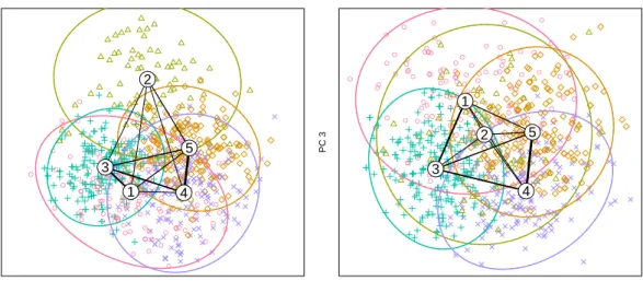
Figure 7 shows the neighborhood graph corre-sponding to the 5 cluster neural gas solution pro-jected into the spaces spanned by PC1 & PC2, and PC1 & PC3, respectively. Colors and plot-ting symbols for the data points are different for each cluster, yet no clear structure can be seen for most parts of the plots. The only struc-ture that can easily be seen is that cluster 2 is “on top” of the left panel. The remaining four clusters all have regions with higher den-sity, but this is not easily seen and the ellipses have large overlapping regions. An obvious (yet overhasty) conclusion would be that the princi-pal component projection obscures the partition
● ● ● ● ● ● ● ● ● ● ● ● ● ● ● ● ● ● ● ● ● ● ● ● ● ● ● ● ● ● ● ● ● ● ● ● ● ● ● ● ● ● ● ● ● ● ● ● ● ● ● ● ● ● ● ● ● ● ● ● ● ● ● ● ● ● ● ● ● ● ● ● ● ● ● ● ● ● ● ● ● ● ● ● ●● ● ● ● ● ● ● ● ● ● ● ● ● ● ● ● ● ● ● ● ● ● ● ● ● ● ● ● ● ● ● ● ● ● ● ● ● ● ● ● ● ● ● ● ● ● ● ● ● ● ● ● ● ● ● ●1 2 3 4 5
Principal Components 1 & 2
PC 1 PC 2 ● ● ● ● ● ● ● ● ● ● ● ● ● ● ● ● ● ● ● ● ● ● ● ● ● ● ● ● ● ● ● ● ● ● ● ● ● ● ● ● ● ● ● ● ● ● ● ● ● ● ● ● ● ● ● ● ● ● ● ● ● ● ● ● ● ● ● ● ● ● ● ● ● ● ● ● ● ● ● ● ● ● ● ● ● ● ● ● ● ● ● ● ● ● ● ● ● ● ● ● ● ● ● ● ● ● ● ● ● ● ● ● ● ● ● ● ● ● ● ● ● ● ● ● ● ● ● ● ● ● ● ● ● ● ● ● ● ● ● ● ● 1 2 3 4 5
Principal Components 1 & 3
PC 1
PC 3
Figure 7: Neighborhood graph for the automobile data with 95% confidence ellipses for the clusters. and a better projection is necessary to see the
data structure (if possible at all).
Figure 8 shows the same neighborhood graph with convex hulls of the clusters and no point symbols. The shaded areas correspond to the convex hulls of the inner 50% of each cluster, the dashed lines to the convex hull of all points within 2.5 median distance from the centroid. Again, the left panel basically differentiates be-tween cluster 2 and the rest. In the right panel the convex hull of cluster 2 has been omitted because it is in the middle and overlaps with all other clusters. It can clearly be seen that the re-maining four clusters divide the space spanned by PC1 and PC3 into 4 regions approximately corresponding to high/low values on x- and y-axis. There is overlap due to projection, but there are also large “pure” regions. Together with the projected axes of the original variables from Figure 6 one could now proceed to con-struct a perceptual map for marketing purposes. Of course, the overlap of the ellipses in Fig-ure 7 can be reduced by only using 50% confi-dence regions, and not plotting point symbols would also make for a “clearer picture”. How-ever, Figure 8 shows that the confidence regions of the clusters are not elliptical and that espe-cially the centroids are nowhere near the “mid-dle” of their clusters. So smaller ellipses would have less overlap, but they would simply shade the wrong region in the plot.
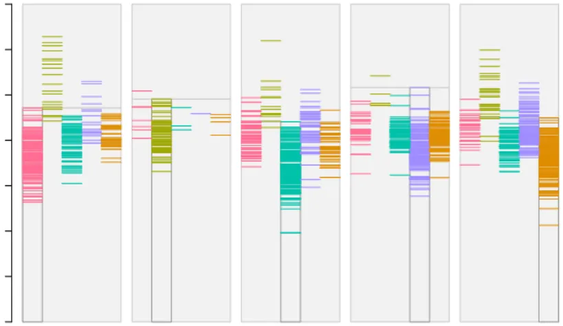
Figures 9 and 10 show stripes and shadow
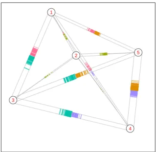
plots for the automobile data, respectively. The interpretation is the same in both cases, all points are “far away” from their cluster cen-troids, none of the clusters is well-separated from the rest. All shadow values are large, the points have similar distances to the closest and second-closest centroid. The shadow star in Fig-ure 11 can be used to identify which segments are more similar to each other than others. All together confirm once more that our grouping is artificial, we have constructed market segments rather than found naturally existing ones.
Note that how the high dimensional data are projected into 2 dimensions is not a focus of this work. We used principal component analysis in this example, but other projection methods like the asymmetric projections by Hennig (2004) would work equally well.
8 Example 2: German
Elec-tions
As second example we use the German parlia-mentary elections of September 18, 2005. The data consist of the proportions of “second votes” obtained by the five parties that got elected to the Bundestag (the first chamber of the Ger-man parliament) for each of the 299 electoral districts. The data set is directly available in R package flexclust. The “second votes” are actually more important than the “first votes”
1 2
3
4 5
Principal Components 1 & 2
PC 1 PC 2 1 2 3 4 5
Principal Components 1 & 3
PC 1
PC 3
Figure 8: Neighborhood graph for the automobile data with convex hulls for the clusters: data points are omitted, the inner convex hull is shaded.
0 0.5 1 1.5 2 2.5 3 3.5
distance from centroid
1 2 3 4 5
Figure 9: Stripes plot for the automobile data, only distances to closest and second-closest centroid are shown.
1 2 3 4 5
●
●
●
●
●
1 2 3 4 5Figure 11: Shadow-stars for the automobile data. because they control the number of seats each
party has in parliament. Before election day, the German government comprised a coalition of Social Democrats (SPD) and the Green Party (GRUENE); their main opposition consisted of the conservative party (Christian Democrats, UNION) and the Liberal Party (FDP). The lat-ter two intended to form a coalition aflat-ter the election if they gained a joint majority, so the two major “sides” during the campaign were SPD+GRUENE versus UNION+FDP. In addi-tion, a new “party of the left” (LINKE) can-vassed for the first time; this new party con-tained the descendents of the Communist Party of the former East Germany and some left-wing separatists from the SPD in the former West Germany. A projection of the data onto the first two principal components is shown in the left plot of Figure 12. The point cloud in the lower left corner mainly correspond to districts in eastern Germany, where support for LINKE was strong, while the upper diagonal cloud cor-responds mainly to districts in western Germany and contrasts the support for the two major par-ties: SPD (up) versus UNION (down). The final outcome of the election was UNION (226 seats in parliament), SPD (220), FDP (61), LINKE (54), and GRUENE (51). UNION and SPD formed a “large coalition” (“große Koalition”), because none of the above mentioned prefer-ences had a majority.
The right panel of Figure 12 shows a four cluster solution from the k-means algorithm.
Cluster 1 captures eastern Germany, while clus-ters 2–4 break western Germany in three parts. The principal component projection shows the structure of the data rather accurate, which makes it easier to relate the new plots intro-duced in this paper to the real structure of the data. The stripes plot in Figure 13 nicely shows the relations between the clusters: cluster 1 is far away from the rest, while cluster 3 is located “between” clusters 2 and 4.
Figure 14 shows another variant of the stripes plot. Here we are not interested in the rela-tive locations of the clusters with respect to each other, but in a categorical background variable. In this case we have highlighted all 45 electoral districts from Bavaria. These are mainly in clus-ter 2, and approx. one quarclus-ter is in clusclus-ter 3. We also see that the Bavarian districts in cluster 3 are not close to the centroid, but have medium distance to it. Finally, Figure 15 shows shadow violins. Again it can clearly be seen that ter 1 is well separated from the rest, while clus-ters 2–4 form a continuum. It also shows that cluster 1 is closer to 3 and 4 than to cluster 2.
Of course, most of the information contained in Figures 13–15 can also be seen in the linear projection in Figure 12 (which is the reason we have chosen this particular example in the first place). However, the stripes plot is independent from the dimensionality of the input space and works also when simple projections of the data like PCA fail.
● ● ● ● ● ● ●●●● ● ● ● ● ● ● ● ● ● ● ● ● ● ● ● ● ● ● ● ● ● ● ● ● ● ● ● ● ● ● ● ● ● ● ● ● ● ●● ●●● ● ● ● ● ● ● ● ● ● ● ● ● ● ● ● ● ● ● ●● ● ● ● ● ● ● ● ● ● ● ● ● ● ● ● ● ● ● ● ● ● ● ● ● ●● ● ● ● ● ● ● ● ● ● ● ● ●●● ● ● ● ● ● ● ● ● ● ●● ● ● ● ● ● ● ● ● ● ● ●● ● ● ● ● ● ● ● ● ●● ● ● ● ● ● ● ● ● ● ● ● ●● ● ● ● ● ● ● ● ● ●● ● ●●● ● ● ● ● ● ● ● ● ● ● ●● ● ● ● ●● ● ● ● ● ● ● ● ● ● ● ● ● ● ● ● ● ● ● ● ● ● ● ● ● ● ● ● ●● ● ● ● ● ● ● ● ● ● ● ● ● ● ● ● ● ● ● ● ● ● ● ● ● ● ● ● ● ● ● ● ● ● ●● ● ● ● ● ● ● ● ● ● ● ● ● ● ●● ●●● ● ●● ● ● ● ●● ● ● ● ● ● ● ● ● ●●● ● ● ● ● ● ● ● ● ● PC 1 PC 2 SPD UNION GRUENE FDP LINKE ● ● ● ● ● ● ● ● ● ● ● ● ● ● ● ● ● ● ● ● ● ● ●● ● ● ● ● ● ● ● ● ● ● ● ● ● ● ●● ● ● ● ● ● ● ● ● ●● ● ● ● ● ● ● ● ● ● ● ● ● ● 1 2 3 4 PC 1 PC 2
Figure 12: Principal component biplot of the German election data (left), and a four cluster solution (right). 0 0.1 0.2 0.3 0.4
distance from centroid
1 2 3 4
Figure 13: Stripes plot for the German election data, only distances to closest and second-closest centroid are shown.
0 0.05 0.1 0.15 0.2 0.25
distance from centroid
1 2 3 4
Figure 14: Stripes plot for the German election data, only distances to closest centroid are shown, districts from Bavaria are highlighted.
●
●
●
●
1 2 3 49 Conclusions
We have extended the CLUSPLOT display by Pison et al. (1999) in two directions: Instead of connecting each cluster centroid with all the oth-ers, we connect only neighboring segments and obtain a graph that is more informative about the relative position of the clusters before pro-jecting them into two dimensions. In addition the line width of the edges are proportional to the number of points that are in between the two clusters, such that thick lines connect clus-ters that are poorly separated from each other. For non-elliptical clusters the convex hulls of inner and outer data points can be used as a 2-dimensional equivalent of a boxplot. Especially for larger data sets and partitions that cannot be easily projected into 2-d, plots can be easier to read if the original data points are only in-cluded in lighter colors or completely omitted. While this complexity reduction step is routine when comparing several samples using boxplots, it is much less common for 2-dimensional visual-izations, because one has to impose an ordering ontoR2. For clustered data a natural ordering
exists through the distance of each point from its cluster centroid.
Shadow values can be used as a computation-ally more efficient approximation to silhouette values. Because shadow values are anchored at the cluster centroids, they allow for the defini-tion of a completely new cluster visualizadefini-tion called shadow-stars. Compared with traditional silhouette plots they give not only information on how well a cluster is separated from the oth-ers, but also to which clusters it is close, if any. A natural question when the silhouette of a clus-ter indicates poor separation is to ask which other clusters are close; shadow-stars can help to efficiently encode this information graphically. A next step will be to investigate how these graphical methods can be used to compare dif-ferent clusterings of the same data set with each other. Do different cluster algorithms and/or distance measures produce solutions with more or less overlap?
References
Becker, R., Cleveland, W., and Shyu, M.-J. (1996), “The visual design and control of trel-lis display,” Journal of Computational and
Graphical Statistics, 5, 123–155.
Everitt, B. S., Landau, S., and Leese, M. (2001),
Cluster Analysis, London, UK: Arnold, 4
edi-tion.
Gordon, A. D. (1999),Classification, Boca Ra-ton, USA: Chapman & Hall / CRC, 2 edition. Hartigan, J. A. and Wong, M. A. (1979), “Al-gorithm AS136: A k-means clustering algo-rithm,”Applied Statistics, 28, 100–108. Hennig, C. (2004), “Asymmetric linear
dimen-sion reduction for classification,”Journal of
Computational and Graphical Statistics, 13,
1–17.
Hintze, J. L. and Nelson, R. D. (1998), “Violin plots: A box plot-density trace synergism,”
The American Statistician, 52, 181–184.
Kaufman, L. and Rousseeuw, P. J. (1990),
Find-ing Groups in Data, New York, USA: John
Wiley & Sons, Inc.
Kohonen, T. (1989), Self-organization and
As-sociative Memory, New York, USA: Springer
Verlag, 3 edition.
Kruskal, J. (1977), “The relationship between multidimensional scaling and clustering,” in
Classification and Clustering, ed. J. V. Ryzin,
Academic Press, Inc., New York, pp. 17–44. Leisch, F. (2006), “A toolbox for k-centroids
cluster analysis,” Computational Statistics
and Data Analysis, 51, 526–544.
Leisch, F. (2008), “Visualizing cluster anal-ysis and finite mixture models,” in
Hand-book of Data Visualization, eds. C. Chen,
W. H¨ardle, and A. Unwin, Springer Verlag, Springer Handbooks of Computational Statis-tics, ISBN 978-3-540-33036-3.
MacQueen, J. (1967), “Some methods for clas-sification and analysis of multivariate obser-vations.” inProceedings of the Fifth Berkeley Symposium on Mathematical Statistics and
Probability, eds. L. M. L. Cam and J.
Ney-man, University of California Press, Berkeley, CA, USA, pp. 281–297.
Martinetz, T. and Schulten, K. (1994), “Topol-ogy representing networks,”Neural Networks, 7, 507–522.
Martinetz, T. M., Berkovich, S. G., and Schul-ten, K. J. (1993), ““Neural-Gas” network for vector quantization and its application to time-series prediction,”IEEE Transactions on
Neural Networks, 4, 558–569.
Mazanec, J., Grabler, K., and Maier, G. (1997),
International City Tourism: Analysis and
Strategy, Pinter/Cassel.
Pison, G., Struyf, A., and Rousseeuw, P. J. (1999), “Displaying a clustering with CLUS-PLOT,” Computational Statistics and Data
Analysis, 30, 381–392.
R Development Core Team (2008), R: A lan-guage and environment for statistical
com-puting, R Foundation for Statistical
Com-puting, Vienna, Austria, URL http://www. R-project.org, ISBN 3-900051-07-0. Rousseeuw, P. J. (1987), “Silhouettes: A
graph-ical aid to the interpretation and validation of cluster analysis,”Journal of Computational
and Applied Mathematics, 20, 53–65.
Rousseeuw, P. J., Ruts, I., and Tukey, J. W. (1999), “The bagplot: A bivariate boxplot,”