ESSAYS IN ENERGY AND ENVIRONMENTAL ECONOMICS
A Dissertation by
JONATHAN BARRETT SCOTT
Submitted to the Office of Graduate and Professional Studies of Texas A&M University
in partial fulfillment of the requirements for the degree of DOCTOR OF PHILOSOPHY
Chair of Committee, Steve Puller Committee Members, Mark Hoekstra
Fernando Luco Reid Stevens Head of Department, Timothy Gronberg
August 2018
Major Subject: Economics
ABSTRACT
This dissertation includes three essays related to energy and environmental economics, with an emphasis on policy. Topics discussed pertain to policies aimed at internalizing externalities, or en-couraging adaptation to climate change. I discuss these topics in the context of the transportation sector, natural disaster insurance, and infrastructure policy.
I analyze consumer behavior in a vehicle arms race—where preferences for safety lead to strategic purchases of large vehicles—as a potential contributing factor to the rise in vehicle sizes in the U.S. First, I test for arms race purchasing behavior by exploiting quasi-random next-door neighbor fatalities in fatal car accidents in order to examine how shifts in preferences for safety impact de-mand for heavy vehicles. I find that households neighboring an individual who dies in an accident respond by purchasing significantly larger and safer vehicles than households neighboring some-one who survives an accident. Second, I explore how gasoline taxes counteract arms race behavior by estimating a discrete choice model of vehicle purchases, allowing for consumer preferences on
relativeweight. My specification allows preferences for vehicle size to vary based on the size of cars in the households’ area. Counterfactual simulations illustrate that an arms race can be reversed with a sufficiently high Pigouvian tax, which will depend on the distribution of vehicle weights, specific to the area.
The next study examines the unintended role government policies can play in discouraging climate change adaptation. Despite the large costs of covering flood losses, little is known about whether flood insurance availability affects the decision to live and stay in more flood-prone areas. In this paper, we present evidence that suggests households in flood-prone areas would have otherwise moved to less risky areas absent flood insurance availability. We identify the effect of flood insur-ance availability on population flows by exploiting the within- and across-county variation in the various programs that the federal government implemented to encourage flood-prone areas to join
the National Flood Insurance Program (NFIP). Results suggest that flood insurance availability caused population to increase by 4 to 5 percent in high flood-risk counties. Furthermore, we find that NFIP causes a 4.4% increase in population per one standard deviation increase in risk.
Finally, I analyze how infrastructure policy may encourage coal plants to convert to clean nat-ural gas energy. The U.S. Environmental Protection Agency’s (EPA’s) Mercury and Air Toxics Standards (MATS) have imposed significant costs on coal-fired power plants in recent years. To many old, inefficient coal plants, high costs of compliance have prompted a trend toward con-versions to natural gas—a much cleaner source of energy. Transportation frictions may inhibit some of these conversions from taking place. In this paper, I analyze the role that the natural gas pipeline infrastructure plays in incentivizing these conversions. Exploiting MATS’ increased pressure on coal electric generating units (EGUs) with capacity 25 megawatts or greater within a triple-differences framework, I estimate that a 10% reduction in pipeline distance produces an additional 6.4% increase in likelihood of conversion for an EGU regulated under MATS. Isolating the impact of pipeline costs within a dynamic model of the plant’s decision to convert (still fully exploiting MATS), I find that pipeline subsidies alone can produce one-third of the conversions as emissions reduction mandates under MATS, and present value of external benefits of $10.1 billion from reduced emissions. In addition, I estimate a marginal benefit of $2.6 million per-mile of pipeline.
ACKNOWLEDGMENTS
I am grateful to my committee chair, Steve Puller, for his continued guidance and support. If not for his valuable advice and encouragement I would not be where I am today.
I am grateful to my dissertation committee: Mark Hoekstra, Fernando Luco, and Reid Stevens for further research advice and support. Additionally, I thank everyone in the applied microeconomics group at Texas A&M for comments throughout countless seminars.
CONTRIBUTORS AND FUNDING SOURCES
Contributors
This work was supported by a dissertation committee consisting of Professors Steve Puller, Mark Hoekstra, and Fernando Luco of the Department of Economics, and Professor Reid Stevens of the Department of Agricultural Economics.
The analysis in Section 3 was conducted in part by Abigail Peralta of the Department of Economics at Texas A&M.
All other work conducted for the dissertation was completed by the student independently.
Funding Sources
Graduate study was supported by assistantships from Texas A&M University, a research fellowship from Strata Policy, and a dissertation research fellowship from Texas A&M University.
TABLE OF CONTENTS
Page
ABSTRACT . . . ii
ACKNOWLEDGMENTS . . . iv
CONTRIBUTORS AND FUNDING SOURCES . . . v
TABLE OF CONTENTS . . . vi
LIST OF FIGURES . . . ix
LIST OF TABLES. . . xi
1. INTRODUCTION . . . 1
2. ARMS RACE DYNAMICS IN VEHICLE PURCHASES. . . 4
2.1 Introduction. . . 4
2.2 Empirical Framework . . . 11
2.2.1 Quasi-experimental Evidence of Purchase Response to Shocks to Prefer-ences for Safety . . . 13
2.3 Data . . . 14
2.3.1 Summary Statistics . . . 16
2.4 Quasi-Experimental Evidence of Arms Race Dynamics . . . 17
2.4.1 Effect of a Neighbor’s Fatality . . . 17
2.4.2 Different Neighbor Samples . . . 19
2.4.3 Dynamic Treatment Effects . . . 19
2.4.4 Placebo Tests . . . 19
2.5 Spillover Effects of Crash Vehicle Weights . . . 20
2.5.1 Results and Robustness . . . 22
2.6 Consumer Preferences in a Vehicle Arms Race . . . 24
2.6.1 The Model . . . 24 2.6.2 Estimation. . . 27 2.6.2.1 Instruments . . . 30 2.6.3 Results . . . 33 2.7 Counterfactuals . . . 35 2.8 Conclusion. . . 40
3. MOVING TO FLOOD PLAINS: THE UNINTENDED CONSEQUENCES OF THE NATIONAL FLOOD INSURANCE PROGRAM . . . 42
3.1 Introduction. . . 42
3.2 Background . . . 46
3.3 Empirical Strategy . . . 48
3.4 Data . . . 52
3.4.1 Population. . . 52
3.4.2 National Flood Insurance Program . . . 53
3.4.3 Other Data . . . 54
3.5 Results . . . 55
3.5.1 First Stage Estimates . . . 55
3.5.2 Graphical Evidence . . . 56
3.5.3 The Causal Effect of NFIP on Population Flows . . . 57
3.6 Effects of NFIP, by Risk Severity . . . 59
3.7 Discussion and Conclusion . . . 61
4. DOES THE U.S. PIPELINE INFRASTRUCTURE PROMOTE CLEAN ENERGY USE? EVIDENCE FROM THE EPA’S MERCURY AND AIR TOXICS STANDARDS . . . 63
4.1 Introduction. . . 63
4.2 Pipeline Infrastructure & Data. . . 71
4.2.1 The U.S. Natural Gas Pipeline Infrastructure . . . 71
4.2.2 Data . . . 72
4.3 Reduced Form Evidence of the Role of Infrastructure . . . 75
4.4 Model . . . 79
4.5 Estimation . . . 83
4.5.1 Identification . . . 88
4.5.2 Model Estimates . . . 89
4.6 Evaluating Counterfactual Infrastructure Policies . . . 90
4.6.1 The MATS Policy . . . 94
4.6.2 MATS, with Pipeline Subsidies . . . 97
4.6.3 Subsidized Pipelines, Independent of MATS . . . 98
4.7 Conclusion. . . 100
5. SUMMARY AND CONCLUSIONS. . . 102
REFERENCES . . . 104
APPENDIX A. FIGURES AND TABLES . . . 112
APPENDIX B. SUPPLEMENTAL CONTENT . . . 143
B.1 Fuzzy Matching Accidents to Owners . . . 143
B.2 Factors Contributing to a Trend Break in the Control Group . . . 144
B.3 Additional Outcomes . . . 145
B.4 An Alternative Control Group . . . 148
B.5 Alternative Mechanisms . . . 149
B.7 Counterfactuals with Equilibrium Prices. . . 154
B.8 Alternative Instrumental Variable . . . 158
B.9 Exogeneity of County Flood Risk . . . 161
B.10 Proof of Proposition 1. . . 164
LIST OF FIGURES
FIGURE Page
A.1 U.S. Average Equivalent Test Weight (ETW) . . . 112
A.2 Effect of Neighbor’s Fatality on Household Vehicle Size . . . 113
A.3 Dynamic Estimates for Weight . . . 114
A.4 Distribution of Placebo Estimates on Household Weight . . . 114
A.5 Distribution of Placebo Estimates: Effect of Crash Vehicle Weights (Same Treat-ment Period, Random Neighbor) . . . 115
A.6 Empirical Weight Distributions (as of Dec., 2008) . . . 115
A.7 Counterfactual Mean County Weights (fuel price = $1.665). . . 116
A.8 Counterfactual Mean County Weights (fuel price = $4) . . . 116
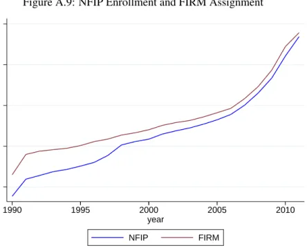
A.9 NFIP Enrollment and FIRM Assignment . . . 120
A.10 Distribution of FHBM Counties . . . 120
A.11 Distribution of Flood Risk Across Counties . . . 121
A.12 Relationship Between FHBM and Flood Risk . . . 121
A.13 First Stage: The Effect of FEMA Intervention on NFIP Enrollment . . . 122
A.14 Event Study Specification of Impact of (Endogenous) NFIP: Naïve Specification . . . . 123
A.15 Event Study Specification of Intent to Treat of NFIP . . . 124
A.16 Placebo Estimates . . . 125
A.17 Heterogeneous Effects of NFIP, by Flood Risk . . . 126
A.18 Coal Generating Unit Initial Year of Operation . . . 130
A.19 Nameplate Capacity (MW) Distribution for Original Coal-Fired Units . . . 130
A.21 Power Plants Under MATS and the Natural Gas Pipeline Infrastructure . . . 132
A.22 Effect of MATS on EGU Conversions . . . 133
A.23 Effect of MATS on Coal EGU Conversions, by Pipeline Proximity. . . 134
A.24 Model Fitted Values of Below/Above Median Distance . . . 134
A.25 Policy Experiment: MATS + Fully Subsidized Pipelines . . . 135
A.26 Policy Experiment: No MATS + Fully Subsidized Pipelines . . . 135
B.1 Effect of Neighbor’s Fatality on Household Vehicle Size, Conditional on Month-of-Sample Fixed Effects . . . 145
B.2 Effect of Neighbor’s Fatality on Other Outcome . . . 147
B.3 Dynamic Estimates for Weight: Treatment Neighbors≥10 as Control . . . 149
B.4 Effect of Neighbor’s Fatality on Fleet Price . . . 151
B.5 Effect of Neighbor’s Fatality on Fleet Price, Conditional on Fleet Size . . . 152
B.6 Optimal Gas Tax to Internalize the Arms Race (fuel price = $1.665) . . . 153
B.7 Optimal Gas Tax to Internalize the Arms Race (fuel price = $4) . . . 154
B.8 Counterfactual Mean County Weights with Equilibrium Prices (fuel price = $1.665) 156 B.9 Counterfactual Mean County Weights with Equilibrium Prices (fuel price = $4) . . . 157
B.10 Log-Difference in CO2/mile Emissions of New Purchases (fuel price = $1.665). . . 158
LIST OF TABLES
TABLE Page
A.1 Summary Statistics . . . 117
A.2 Effect of Neighbor’s Fatality on Household Vehicle Size (two nearest neighbors) . . . . 117
A.3 Effect of Neighbor’s Fatality, by Neighbors . . . 118
A.4 Spillover Effects of Crash Vehicle Weights . . . 118
A.5 Spillover Effects of Crash Vehicle Weights, by Neighbors . . . 119
A.6 Logit Demand Estimates . . . 119
A.7 County Characteristics . . . 127
A.8 First Stage: NFIP enrollment on FIRM and FHBM assignment . . . 127
A.9 Effect of Flood Insurance on Migration (Reduced Form) . . . 128
A.10 Heterogeneous Effects of NFIP on Migration, by Flood Risk . . . 129
A.11 Summary Statistics . . . 136
A.12 Effect of Pipelines on Conversions Under MATS (OLS) . . . 137
A.13 Effect of Pipelines on Conversions Under MATS (WLS) . . . 138
A.14 Maximum Likelihood Estimates . . . 139
A.15 Effect of Converted Capacity on Emissions . . . 140
A.16 MATS Model Predictions . . . 141
A.17 Policy Counterfactual: MATS, with Subsidied Infrastructure . . . 141
A.18 Policy Counterfactual: Subsidized Infrastructure, without MATS. . . 142
B.1 Effect of Neighbor’s Fatality in a Vehicle Accident . . . 148
B.2 Effect of Neighbor Dying on Vehicle Price . . . 151
B.4 Effect of FIRM on Migration . . . 160 B.5 Effect of NFIP on County Floods . . . 162 B.6 Heterogeneous Effects of NFIP on Migration Using Residualized Floods (2SLS) . . . . 163 B.7 Effect of Conversions on Plant Generation Levels . . . 166
1. INTRODUCTION
Externalities are a primary driver of market inefficiencies. These externalities are often produced as a byproduct to consumer, producer, or even government behavior pertaining to market activi-ties. In this dissertation, I study environmental externalities produced by each one of these entiactivi-ties. The emphasis in this research is on policy solutions which would internalize some or all of the external costs produced by these actions. In each of the following chapters, I study and/or offer policy solutions to these environmental externalities, in order to achieve more efficient economic outcomes. This analysis will concentrate on three sectors: transportation, government subsidized flood insurance, and electricity.
In Chapter 2, I examine costly externalities produced by vehicle consumers in the transportation sector. Specifically, I study one potential mechanism which has caused increases in the size of the fleet in the past several decades. This factor—described as a vehicle arms race—occurs when consumers strategically purchase larger vehicles in order to protect themselves from other cars on the road. These strategic responses are, therefore, a function of consumer preferences for safety. The literature on the vehicle arms race is quite sparse, and there is little to no causal evidence of these “arms race"-stylepreferences. In this chapter, I isolate shocks to preferences for safety in the form of household responses to the death of anext-door neighbor in a vehicle accident. Using a unique household-level dataset with exact addresses, I exploit the quasi-random nature of a neigh-bor’s fatality using within household variation in purchases. My estimates suggest that households respond to this shock to preference for safety by increasing their vehicle sizes significantly over time. Since in a vehicle arms race, these preferences for safety are presumably linked to the size of other vehicles on the road—generating feedback loops in fleet size—I directly examine this re-lationship within a discrete choice model of vehicle purchases. Specifying preferences for vehicle size as a function of consumers’ local distribution of vehicle weights in their area allows me to estimate the impact of several counterfactual policy interventions which would serve to internalize
this feedback loop. I examine a Pigovian gas tax and illustrate that with a sufficiently high tax an arms race can be reversed. That is, raising gasoline prices via a tax induces households to purchase more fuel efficient (i.e., smaller) vehicles, which reduces the size of vehicles on the road, and thus induces the next round of purchasers to buy smaller cars.
In Chapter 3, co-author Abigail Peralta and I look at federally subsidized flood insurance from the National Flood Insurance Program (NFIP), and analyze the impact of the poor incentives it produces. In the face of rising sea levels and increased risk of flood, adaptation may be a natu-ral response for households. For example, households might adapt by migrating out of the areas that are more susceptible to flood. However, when faced with highly subsidized flood insurance, being compensated for potential losses could shift households on the margin away from moving out of a flood-zone. We estimate a treatment effect of receiving NFIP on the population of the treated, risk-prone areas of the U.S. In this chapter, we exploit within- and across-county variation in various, plausibly-exogenous, programs that the federal government implemented to encourage flood-prone areas to join the NFIP. We demonstrate that the counterfactual response—in absence of flood insurance take-up—would be a decline in the population of these high flood-risk areas. Specifically, we estimate that NFIP is responsible for a 4 to 5 percent increase in population in high flood-risk counties. In addition, we study the differential effects of subsidized flood insurance availability based on local area’s relative flood risk. We find that NFIP causes a 4.4% increase in population per on standard deviation in risk. This finding suggests that NFIP contributed to a 6.6% increase in costs attributed to hurricane Katrina, and up to a 15% increase in costs associated with hurricane Harvey. The moral hazard produced by the NFIP, and uncovered in this chapter, provides strong evidence that premiums are much too low in the country’s most flood-prone areas.
Chapter 4 of this dissertation studies the costly externalities produced by the country’s coal-fired power plants, and looks to infrastructure as a possible factor that could reduce these external costs. This chapter examines the relationship between the natural gas pipeline infrastructure and natural
gas usage. Newly imposed regulations, such as the Environmental Protection Agency’s (EPA’s) Mercury and Toxics Standards (MATS), have placed significant costs on power plants generating electricity from coal or oil. The primary option for the affected plants is to invest in costly equip-ment to achieve compliance. However, a recent trend is the conversion from coal or oil to natural gas fired-burners. These transitions to natural gas usage have enormous environmental benefits, as burned natural gas emits about half the carbon dioxide of coal. In this chapter, I exploit as-good-as-random variation in MATS treatment—imposed on coal and oil electric generating units (EGUs) of 25 megawatts or greater—in order to estimate the influence that proximity to pipeline has on the plants’ decision to convert an EGU subject to MATS. The estimates presented in this chapter demonstrate that MATS creates significantly larger incentives for coal plants to convert to natural gas when the plant is in close proximity to the pipeline network. Specifically, I find that a 10% reduction in pipeline distance produces an additional 6.4% increase in likelihood of conver-sion for a generating unit subject to MATS. I examine these incentives more thoroughly within a structural framework, which allows me to isolate the contribution of pipeline proximity to a coal plant’s fixed cost of conversion. This dynamic model of the plant’s decision to convert allows me to estimate the impact of infrastructure as a potential policy lever for clean energy use, even in absence of MATS. Model estimates demonstrate large-scale benefits from pipeline subsidies that amount to nearly one-third the benefits of federal mandates through MATS. These results sug-gest that pipeline subsidies alone can lead to present value external benefits of up to $10.1 billion in emissions reductions from coal-to-natural gas conversions. Additional calculations estimate a marginal value of the pipeline infrastructure at $2.6 million per-mile.
2. ARMS RACE DYNAMICS IN VEHICLE PURCHASES
2.1 Introduction
The average size of the U.S. vehicle fleet has risen steadily over the years. According to the Na-tional Highway Traffic Safety Administration (NHTSA), passenger cars have observed a 12.5% increase in weight, and light trucks a 26% in weight from model year 1984 to 2004. This increase in vehicle sizes can be seen in Figure A.1. With vehicles on the road contributing to nearly one-fifth of carbon emissions, and the negative relationship between vehicle size and fuel efficiency, this growth in fleet size has added significantly to the increase in carbon emissions over the years, and has impeded much of the progress in fleet fuel efficiency.
The increased size of the vehicle fleet is driven by multiple factors. Consumers throughout most of this period have experienced growths in income, so an increased willingness to pay for vehicle size might explain a portion of the growth in fleet size. The increase in fleet size may also be driven by relatively low real prices of fuel, reducing the cost of driving these large cars. This paper ex-amines another factor contributing to the growth in fleet size: consumers strategically responding to heavy cars on the road, thereby increasing their purchases of sport utility vehicles (SUVs) and pickup trucks, relative to passenger cars, in order to “protect" themselves from other vehicles on the road. Anderson and Auffhammer (2014) demonstrate that large weight disparities in two-car collisions significantly increase the likelihood of a fatality occurring. Their work documents the fact that “pounds kill," however, no research has shown whether consumers incorporate the fact that “pounds kill" into their purchase decisions. This paper seeks to answer the question of whether consumers know that “pounds kill" and purchase accordingly.
Households may purchase larger vehicles due to preferences for safety. The same household may prefer a larger vehicle if the cars owned by other households in the area are larger. The literature
on the vehicle “arms race” (e.g., White, 2004; Li, 2012) discusses these preferences for safety, wherein consumers buy increasingly large vehicles to protect themselves from other cars on the road. This type of contagion effect, inherent in a vehicle arms race, produces higher emissions and increased risk on the road as vehicles increase in size. Furthermore, these responses create feedback loops that cause the fleet to be heavier than it would otherwise be, absent the strategic motive by households to protect themselves.
The traditional view is that heavier vehicles provide more safety when experiencing an accident (Crandall and Graham, 1989). However, consumers who protect themselves by purchasing pickup trucks and SUVs create an increased risk on the road to other drivers. It is well-documented that large vehicles create an increased risk of fatality to the opposing driver when involved in an acci-dent. For example, Jacobsen (2013) finds that a 1,000 pound increase in the weight of a vehicle involved in an accident increases the number of fatalities in other vehicles by about 46 percent, but reduces own risk by 53 percent. Anderson and Auffhammer (2014) find, conditional on the occur-rence of an accident, a 1,000 pound increase in vehicle weight is associated with a 47% increase in the baseline fatality probability. Evans (2001) finds that the effects of adding mass, in the form of a passenger, adds to the increased risk of fatality in head on collisions. He finds that adding a passenger to a car leads to a 7.5% reduction in driver’s risk of fatality, while increasing the risk of fatality to the other driver by 8.1%. Bento et al. (2017), similar to Anderson and Auffhammer (2014), examine the relationship between weight dispersion and fatalities in accidents, but in the context of CAFE. They find that, though CAFE increased the national fleet’s weight dispersion, the resulting decrease in average weight produced an overall reduction in fatalities.
These types of safety attributes, and the extent to which consumers understand the relationship between size and safety, may create strong preferences forrelativelylarge vehicles. To my knowl-edge, no prior research has provided causal evidence that households respond to heavier vehicles they encounter on the road by purchasing larger cars. I examine this relationship in this paper.
Furthermore, I show that these arms race dynamics are a significant determinant of the increasing fleet size. Finally, I demonstrate how Pigouvian taxes, when accounting for an arms race, may counteract these types of preferences.
The types of incentives uncovered in this paper have significant externalities. For example, because larger cars tend to be less fuel efficient, increased demand for heavier vehicles has a conflicting effect on policies seeking to improve vehicle fuel economy. CAFE standards aim to reduce en-ergy consumption by increasing the fuel economy of the U.S. vehicle fleet through manufacturer targeted minimum fuel efficiency requirements. The CAFE standards have had positive effects on improving average vehicle miles-per-gallon (MPG), however, the vehicle arms race creates an opposing dynamic, reducing the overall potential of CAFE.
Accounting for the dynamic preferences for weight, inherent in an arms race, is especially impor-tant when evaluating Pigouvian taxes. For example, a tax on gasoline which takes into account consumers’ static preferences for large vehicles ignores how these preferences might change in response to other cars on the road. In an arms race, consumers favor large cars increasingly more as the fleet size around them grows. Not accounting for these dynamic preferences can lead to mis-estimation of a tax. Thus, credible identification of arms race preferences is an important step in improving these policies.
Industry analysts have conjectured that an arms race effect has played a major role in the growth in size of the vehicle fleet presented in Figure A.1. The logic is captured in a New York Times article on the “SUV Arms Race," quoting a consumer saying, “I’m sure the world would be a better place if we all drove Minis, but with so many crazy drivers on the road, I want the biggest vehicle I can get."
credible evidence that this type of behavior actually exists. A primary reason is the difficulty in identifying such an effect using naturally occurring field data. The thought experiment would be to randomly assign households in some region with large vehicles and another region with small vehicles, and observe the weights of future car purchases. Such an experiment would isolate con-founding factors such as common shocks and unobserved characteristics that are common across households, and also reveal preferences for vehicle size. Random assignment would also mitigate concerns of simultaneity bias; we would be able to properly identify the causal direction of the treated households impact on other households. However, such large scale experiments are often infeasible in practice.
In this paper, I exploit a source of quasi-random variaton in treating households with a salient shock to consumers’ preceptions about vehicle safety. Specifically, I compare the behavior ofnext-door
neighbors of households that were involved in a serious accident. To explain, consider a two-car collision, in which the driver of one car dies and the driver of the other car survives. This accident is a salient information shock to acquaintancesof the drivers involved in the accident, and may impact the future vehicle purchase behavior of those acquaintances. To proxy for unobserved ac-quaintances in these crash victims’ networks, I compare the subsequent vehicle purchase behavior of the next-door neighbors of the drivers who died to the purchase behavior of the next-door neigh-bors of the drivers who survived.
I use a difference-in-differences empirical strategy to measure the impact of this salient preference shock. To implement this strategy, I use a rich administrative database of vehicles registered in Texas from 2004-2010, matched to a census of all vehicle accidents in Texas. Using a panel of household-level vehicle purchase data, I study the changes in the weights of the neighbors’ vehicle purchases after the accident. I find that prior to the accident, the next-door neighbors purchased vehicles with extremely similar weights. However, after the accident, the next-door neighbors of the driver who died in the accident owned vehicles that were 20-30 pounds heavier than the
next-door neighbors of the driver who survived (see Figure A.2). This amounts to roughly one in ten treated households upgrading from a sedan to a mid-sized SUV.
I exploit another source of quasi-random variation to verify these vehicle purchase dynamics. I study two-car accidents, where it has been shown that increases in weight of the striking vehicle will increase the fatality risk of passengers in the smaller vehicle (Anderson and Auffhammer, 2014). I show that when a victim is quasi-randomly hit by a heavy vehicle, and the victim is driving a smaller vehicle, the next-door neighbor responds by purchasing a larger car, following the accident. This exercise provides further evidence that a salient shock to preferences for safety results in higher demand for large vehicles.
I consider these responses by consumers to be evidence of information shocks to their perceptions of vehicle safety. This is primarily due to the salient information that these households are treated with. That is, a household now becomes aware of an acquaintance’s fatality in an accident. This type of information evidently creates an adjustment in preferences for vehicle attributes related to safety. The primary determinant of these changes in preferences is plausibly due to a change in beliefs about the safety of their current vehicles.
In this paper, I do not take a stand on potential behavioral mechanisms that could be driving these changes in preferences. One can speculate that these responses may be a result of projection bias (Lowenstein et al., 2003; Conlin et al., 2007; Busse et al., 2014), anchoring heuristics (Slovic, 1967; Tversky and Kahneman, 1974; Crandall and Graham, 1989; Furnham, 2011), or other as-similative biases. Identifying any behavioral mechanisms that may be driving these responses is not feasible given the information that I have. Furthermore, I cannot reject the possibility that consumers are simply rationally updating beliefs from incorrect priors.
race dynamics affect vehicle purchases. It is important to understand how these preferences will impact the evolution of the vehicle fleet over time, and how policies might operate to internalize an arms race. To do so, I use a discrete choice model to directly estimate revealed preferences for vehicle size, as a function of the vehicle fleet around a consumer. This model allows me to simulate the long-term effects of an arms race feedback loop under various counterfactual policy schemes.
I estimate a discrete choice logit model of vehicle purchase that allows tastes for vehicle weight to vary based on the distribution of vehicle sizes in a consumer’s local area. This model directly estimates consumer preferences, and thus, I will be able to place a dollar value onrelativevehicle weight. That is, I consider how shifts in vehicle sizes within an area change how consumers value their own vehicle size. In order to estimate this model, I need to account for the possibility that unobservered preferences for weight are correlated with the weight distribution in a consumer’s area. To do so, I devise a unique instrument based on the variation in past gasoline prices, in-ternalized by consumers at past times of purchase, as well as beliefs about future gasoline prices (Anderson et al., 2012). Results indicate that a consumer’s value of an additional pound of weight increases by $0.02 following a one pound increase in average county vehicle size. This implies a consumer would value a Jeep Cherokee (SUV) about $3,200 more than a Honda Accord (sedan), when treated with a county driving all Ford Explorers (heavy county), compared to a county driv-ing all Ford Fusions (light county).
Finally, I use the model to calculate the impact of counterfactual events, such as a sustained pe-riod of very low, or very high gas prices. This exercise provides insight into the impact of static Pigouvian taxes in an arms race. I find that, with sufficiently high gas prices, an arms race can be reversed. That is, if consumers find it too costly to increase vehicle size, weight distributions shift downward, and thus, consumers are less endangered by the relatively lighter vehicles on the road. With high gas prices sustained for long periods of time, consumers have a lower likelihood of be-ing harmed by the previously purchased, smaller vehicles on the road, and therefore benefit from
reducing vehicle sizes further. This creates a downward spiral in vehicle sizes with large environ-mental benefits. However, when gas prices are low, the arms race feedback loop is exacerbated, which leads to substantial increases in fleet size. Since consumers internalize their preferences for weight and preferences for safety—which depend on the size of their local fleet—the optimal Pigouvian tax to internalize an arms race will ultimately depend on the local weight distributions.
These exercises illustrate the importance that optimal tax calculations take into account consumers’ dynamic preferences for vehicle size. Taxing schemes may differ based on the policy objective; however, I examine a tax to fully internalize an arms race feedback loop. Simulation results indi-cate, to fully internalize an arms race, in many instances, it is most efficient to stimulate a reduction in vehicle size with an initial tax rate increase, kick-starting a reverse arms race, then following up with a tax reduction. The initial tax increase serves to replace many of the large cars on the road with smaller cars, due to the increased price of driving large vehicles. This ultimately shuts off much of the feedback loop, as consumers grow less concerned for safety when the vehicles around them drop in size. Once the arms race has been neutralized, estimates indicate it is efficient for taxes to drop.
The evidence of a vehicle arms race I present in this paper provides new evidence of a major factor driving the increases in fleet size over the years. These preferences exist even in the presence of government standards, such as CAFE, that aim to improve fuel efficiency, and thus, place down-ward pressure on the size of the fleet. These types of strategic responses by consumers therefore identify a new dynamic which policy efforts must account for when designing policy.
No policy would be able to eliminate the type of preferences that I uncover in this paper. How-ever, internalizing some of the externalities produced in an arms race can significantly weaken the growth in fleet size produced by this feedback loop. This paper specifically looks at a gas tax as a potential policy lever to moderate the growth in vehicle size. When it becomes too costly to drive
trucks and SUVs, consumers will respond by purchasing smaller, more fuel efficient cars, which weakens the best response mechanisms of subsequent purchasers. Though not directly examined in this paper, a feebate—some combination of fees and rebates—implemented in the market for new vehicles may also produce a more efficient outcome. It is important to note, that any policy addressing the costly externalities produced by arms race preferences, must take into account the feedback loops generated when consumers respond in purchases to other vehicles on the road.
The paper proceeds as follows: In Section 2.2, I lay out the groundwork for my empirical identifi-cation strategy. In Section 2.3, I discuss the data and dataset construction. In Section 2.4, I present my primary estimation results of the effect of neighbor’s fatality and a series of robustness checks. In Section 2.5, I provide further quasi-experimental evidence of an arms race by examining the additional impact of large vehicles in vehicle accidents. In Section 2.6, I introduce and estimate a model of consumer choice in an arms race. In Section 2.7, I use the estimated model to calculate the magnitude of an arms race in different Pigouvian scenarios. In Section 2.8, I conclude my paper with a brief discussion of the implications of my findings.
2.2 Empirical Framework
This paper has two specific research questions that will address two distinct aspects of a vehicle arms race. First, I examine how consumer preferences for vehicle safety can drive demand for large cars. That is, I study whether consumers behave in a manner consistent with an arms race, or have arms race-stylepreferences. To identify these responses, I exploit vehicle accidents as an exogenous shifter of preferences for safety. Second, I examine how consumer preferences for ve-hicle size change as a function of the size of veve-hicles on the road, and policies that can internalize arms race externalities. This approach will require a model of vehicle choice, where preferences depend on local distributions of vehicle sizes.
To study consumer preferences for safety in an arms race, I narrow my focus to salient outcomes which large vehicles produce in accidents. Specifically, I studynext-doorneighbors of individuals
involved in fatal accidents. Among those involved in an accident with a fatality, some will live and others will die. Thus, some of the next-door neighbors will be “treated” with the knowledge that someone who they likely knew died in a vehicle accident. I view this treatment as an information shock to consumers’ perception of vehicle safety, which is most likely influenced by the size of the vehicles involved in the accident.
To illustrate how this shock to perceived preferences for safety might impact consumer behavior, consider an additive utility function, where consumers place value on the safety associated with a certain vehicle’s weight. In the spirit of Anderson and Auffhammer (2014), suppose this value enters the utility function negatively in the form of a consumer’s belief about the probability of dying in an accident, conditional on the weight of that vehicle and the distribution of vehicle sizes in the population,f(·). Lethi(wj, w)be a functionproportionalto consumeri’s beliefs about the probability of dying in a vehicle,j, of weightwj, when colliding with another vehicle of weightw (i.e., P r(die in an accident|wj, w)enters utility linearly). Suppose consumer ichooses a vehicle subject to a budget constraint, with the price of a numeraire good normalized to one. Leti’s indirect utility function for vehiclej be described by the following.
uij =αi(yi−pj) +xjβi− Z
hi(wj, w)f(w)dw+εij (2.1)
whereαi describes consumeri’s marginal utility of income,yiisi’s income,pj is the price for car
j, βi are preference parameters on various attributes,xj (may include vehicle size), and εij arei’s unobserved preferences for vehiclej. Suppose consumeriupdates their beliefs ofhi(·)following the death of a neighbor in an accident tohi(wj, w|neighbor_diedi). That is, a neighbor’s fatality increases the saliency of the role that weights play with respect to safety.
or flat in weight (i.e., ∂hi(wj,·)/∂wj = 0 ). Following the neighbor’s death, consumer i up-dates beliefs such that the probability of dying is lower if one is driving a heavier vehicle (i.e.,
∂hi(wj,· |neighbor_diedi)/∂wj <0). Not directly examined in this paper, this updating may be a result of projection bias, incorrect priors, or some other behavioral mechanism. The extent to which the consumer updates these beliefs, conditional on a neighbor dying, governs the extent to which the consumer changes their preferences for safety.
2.2.1 Quasi-experimental Evidence of Purchase Response to Shocks to Preferences for Safety
Evidence of an increased preference for safety following a neighbor’s death can be directly ob-served through the consumers’ revealed preferences for weight. The extent to which consumers adjust these preferences according to the distribution of vehicle sizes on the road, w ∼ f(·), (as in Equation 2.1) is examined directly in Section 2.6. The key focus of the first part of this paper, however, is in isolating these shocks to consumers’ preference for safety.
My empirical strategy to isolate these shocks to preferences for safety is to implement a difference-in-differences estimator of the treatment effect of neighbor’s fatality on household choice of vehicle size. The key identifying assumption is that subsequent vehicle purchasing behavior of the treated group would have followed a parallel pattern of the control group, absent treatment. I test if the two groups are parallel, absent treatment, by testing if trends in outcomes were similar prior to the accident. Specifically, I estimate the following fixed effects regression:
weightit =αi+λt+β·neighbor_diedit+εit (2.2)
whereweightitis the average curb weight of householdi’s fleet in month-of-samplet, andneighbor_diedit is an indicator which equals one if householdidied in a vehicle accident in some periods≤t, and
treated (ATET). As I observe multiple purchases from the majority of households in my sample, I control for household level and month-of-sample fixed effects,αi andλt, respectively.
I will estimate Equation 3.2 using, as my control group, households neighboring an individual who was involved in a fatal accident (at least one crash victim died), but who survived it. The intuition is that this group of individuals will likely behave similar to the treatment group on average. It is likely that the control group had larger vehicles on average than those of the treatment group. This might be the case because of the correlation between vehicle size and likelihood of fatality in an accident, as well as the correlation in characteristics among neighbors. This alone does not violate the identifying assumption. It is only required that these differences remain fixed over time, prior to the accident.
Using the neighbors of the survivorsas the control group could lead to smaller estimates than if the control group included households who had no neighbor experience a car accident at all. This could be the case if the control group was affected (in the same direction) by their neighbor’s ac-cident too, even though that neighbor survived. However, using thesurvivorsas the control group should provide robust estimates because of the presumed similarity they have with the treatment group, but with a distinguishing feature (i.e., surviving) that will help disentangle the effects of a neighbor’s death.1
2.3 Data
The data for this paper are derived from vehicle registrations and accident records. For vehicle accidents, I use information on accidents involving at least one fatality. These data come from the
1One could argue that using thesurvivorsas my control group may make the effect seem larger than it actually is.
This could be the case if the neighbors of these survivors decided to purchase smaller vehicles following the accident. Therefore, to lead to an over-sized estimate of the effect on the treatment group, the control households would need to be unrealistically conscious of the accidents and willing to reduce the size of their vehicle to “save” others’ lives. I view this social utility hypothesis as unlikely to be the case, and thus, posit that my estimates will be a lower-bound of the true effect of treatment. With that said, in the Online Appendix B.4 I explore an alternative control group and demonstrate that my choice of control group does not significantly alter my estimates.
Fatality Analysis Reporting System (FARS) and are supplemented with a Texas A&M Transporta-tion Institute (TTI) dataset, which is a census of police accident reports forallTexas accidents. All accidents data are observed over the years 2006 through 2010. For household vehicle ownership, I use confidential administrative records maintained by the Texas Department of Motor Vehicles (DMV). These data include all registration records for 2004 through 2010.
In this paper, a majority of the analysis will be conducted on neighbors of crash victims. This requires identifying the victims of these crashes in the registrations data. The DMV data provide the exact addresses of these households, given their last vehicle registration. Once I have these addresses, I can locate physical next-door neighbors, by finding households located within the nearest distance, and on the same street.
For each household neighboring a crash victim, I decode the vehicle identification numbers (VIN) for their entire fleet using a database obtained from DataOne Software. These data allow me to merge in various characteristics of each vehicle, such as make, model, year, weight and MSRP. The majority of the analysis in this paper focuses on the size of the households’ vehicle fleets.
Due to an absence of VIN or household-level information in the FARS dataset, I make use of addi-tional information in the TTI data to “fuzzy” match fatal vehicle accident victims to households in the DMV dataset. This process involves two layers of “fuzzy” matching, in which I first match key TTI information to FARS observations, and then match fatal accident victims to vehicle owners in the DMV data. Combining these two datasets provides me with (non-unique) 12-digit substrings of 17-digit VINs, dates of crashes (which provide information on ownership times), as well as the drivers’ first and last name. I proceed by using this information to “fuzzy” match to ownership records in my DMV data.
have information from the DMV dataset such as vehicle ownership and addresses. I locate the neighbors of these households, and their corresponding ownership histories. It is important to recognize that this matching procedure will most likely lead to some measurement error in the treatment variable. That is, I may incorrectly identify a household as being involved in a fatal accident. Estimated treatment effects may, therefore, be attenuated.
For the purpose of estimating the effect of a neighbor’s fatality on nearby neighbors, I will restrict the set of neighbors to those located on the same street as the individual involved in the accident, and within 100 meters. I primarily focus on the two nearest neighbors, but will show robustness through other samples.
2.3.1 Summary Statistics
Summary of statistics are presented in Table A.11. Each column in the table corresponds to a differ-ent sample containing a differdiffer-ent number of nearest neighbors. These are thekclosest households neighboring the individual who experienced a vehicle accident. Note that the sample size is not exactly proportional to the number of nearest neighbors included. This is either the result of miss-ing data, small streets, or neighborhoods with spaced out houses (as only houses on the same street and within 100 meters are included in my dataset).
About 56% of households in my sample are treated with a neighbor fatality. The average vehicle curb weight in this sample is about 3,700 pounds. This is about the mass of a medium-sized SUV. About 67% of households in the sample own at least one passenger car, as opposed to owningall
light trucks.
Another key characteristic of this sample is that the average household purchases just over two vehicles over the course of the seven years of my registrations data (2004-2010). Because of these quite infrequent purchases, any adjustment to household vehicle characteristics will most likely be a slow and gradual process. Note that the fixed-effects estimators in this paper will fully absorb
one-car purchase households, and will only exploit the variation coming from households who purchase multiple vehicles within the time-frame of my data.
2.4 Quasi-Experimental Evidence of Arms Race Dynamics
2.4.1 Effect of a Neighbor’s Fatality
In this section, I look at the effects of these information shocks on various outcomes. Specifically, I test whether a neighbor’s fatality in a vehicle accident has an effect on the revealed preferences for vehicle size.
I examine consumer behavior at the household-level, on a monthly-level panel and estimate Equa-tion 3.2, where the outcome is a snapshot of the size of the household fleet at a given month in time. Note that the characteristics of a household fleet will only change when the household purchases a new vehicle. For these new purchases I observe the exact date, however for simplicity, I collapse these into monthly observations.
Evidence of a treatment effect on neighbor’s death can be seen in Figure A.2. This figure plots the average vehicle size for the treatment and control groups on months away from treatment. I have included only the two nearest next-door neighbors in this figure, though I check the robustness across different samples of neighbors in Section 2.4.2. As expected, the neighbors of those who died tend to track well against the neighbors of the survivors in the periods preceding treatment. At the treatment period, their paths begin to diverge. This figure illustrates that the treatment group begins to increase the relative size of their vehicles following neighbor’s death.
It is apparent that the control group breaks trend around the time of the accident. Note that this should not bias my estimates, so long as my identification strategy is valid—that is, as long as the treatment group would have continued to follow the same trend with the control group, absent a neighbor’s fatality. In Online Appendix B.2, I show that this trend break is entirely generated by
time specific factors2, and thus should not bias my estimates. I also examine an alternative control group in Online Appendix B.4 and confirm similar results.
The parallel paths of the treatment and control groups in Figure A.2 provide strong evidence that I can accurately predict the treatment group’s counterfactual path, absent treatment. Table A.2 presents the least squares estimated treatment effect on household average vehicle weight. The sample includes the nearest two neighbors to the individual involved in the accident.
Column 1 estimates the treatment effect using the traditional difference-in-differences estimator, which controls for a post-accident indicator, as well as a treatment group indicator. In Column 2, I control for time-invariant census tract-level demographic variables, such as median income, percent white, percent black, and median age. Column 3 includes month-of-sample fixed effects, and in Column 4, I estimate Equation 3.2. This includes a full set of household and time fixed effects. Note that these estimates fully absorb any variation coming from households who have no new purchases during the time-frame of my sample. This may explain the decrease in the size of these point estimates after including household-level fixed effects. In the last column, I include a county-specific linear time trend, allowing each county to follow differing trends.
These estimates indicate that households residing near a neighbor who died in an accident, increase their average vehicle size by about 20 to 30 pounds following a neighbor’s fatality. This implies that, for a two-vehicle household purchasing only one new car in the post period, this vehicle should on average be about 40 pounds heavier. This is equivalent to a 400 pound upgrade for one in ten two-car neighbors—roughly the same as a switch from a sedan to a mid-sized SUV.
These estimates suggest that a neighbor’s fatality in a vehicle accident makes vehicle weight salient to these households. This type of behavior is consistent with preferences in a vehicle arms race,
2The median crash time in my data is June 2008. This was a period experiencing very high gas prices—one factor
where the neighbor’s death in a car crash serves as a quasi-random shock to preferences for safety.
2.4.2 Different Neighbor Samples
Next I estimate these treatment effects using different samples of nearest neighbors. In each spec-ification, I include the nearest one throughk nearest next-door neighbors (on the same street), as listed in Table A.3. These estimates serve as a falsification, as one would expect the estimates to become attenuated as I add neighbors who live further away—who are less likely to be acquain-tances with the crash victims.
Examining the results in Table A.3, the two neighbor sample appears to capture the largest effect in terms of household vehicle weight (though not statically different from the three neighbor sample). These neighbors are more likely to be acquaintances with the crash victims than neighbors further away. The estimates show a gradual decay in size following the second neighbor. The effect of neighbor’s fatality is no longer significant by the ten nearest neighbors sample.
2.4.3 Dynamic Treatment Effects
Next, I estimate a fully dynamic version of Equation 3.2. In the regression, I include six leads and twenty-four lagged indicators of treatment. The final lagged term is an indicator for 24 or more months post-fatality—it reflects the remaining time-span of the data. The leading terms serve as placebos, as I should not expect future fatalities to impact current household vehicle sizes. This formally tests the parallel trends assumption, as displayed in Figure A.2. The dynamic treatment effects presented in Figure A.3 also illustrate the gradual effects of neighbor’s fatality on the av-erage weight of the households’ vehicle stock overtime. These estimates indicate that, a year out from the treatment period, treated households are driving vehicles roughly 20–25 pounds heavier.
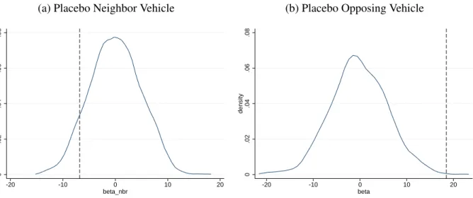
2.4.4 Placebo Tests
I further check the robustness of the findings in Table A.2 by estimating the treatment effect for a series of placebo estimates. This procedure is similar to the one outlined by Bertrand et al. (2004).
Using the same sample as in Table A.2 (two neighbor sample), I randomly assign each of 15,723 households to the treatment or control group, with the same frequency of treatment as the empirical probabilities. I randomly assign a treatment period to each household from the periods in which the household was observed. For most households, I observe their vehicle stock for the duration of the accidents data, which begins in 2006 and ends in 2010. I proceed by estimating Equation 3.2 for these placebo treatments. I repeat this process 1,000 times and record the estimates for each.
This process leaves me with a distribution of placebo estimates. In a manner similar to that of synthetic control methods (e.g., Abadie et al., 2010), I calculate one-tailed p-values for my esti-mates in Table A.2 from the resulting distribution. A kernel distribution of the placebo estiesti-mates is presented in Figure A.4.
As expected, this distribution is centered on zero, which indicates a mean zero effect for a randomly assigned placebo treatment. My estimate for the effect of neighbor’s fatality on average household vehicle weight ranks at the top of the distribution, with a corresponding p-value of 0.3%. This implies that less than half a percent of placebo treatements resulted in a greater estimate than my estimate of 19.95 (from Table A.2), suggesting it is highly unlikely that an effect of this size was estimated by chance.
2.5 Spillover Effects of Crash Vehicle Weights
In this section, I provide further evidence of arms race-stylepreferences by examining how house-holds neighboring crash victims respond indirectly to the size of vehicles involved in the accidents. The idea is that a larger striking (or opposing) vehicle, and a smaller vehicle driven by a neighbor, produces more severe and salient outcomes (Anderson and Auffhammer, 2014). The household neighboring the victim then directly responds to these salient outcomes—a direct function of the crash weights.
Identification of indirect responses to the size of the vehicles involved in these accidents come from the as-good-as-random timing of the accidents. Neighboring households may directly respond to each other’s vehicle size by means of social norms. I will not be able to identify these baseline
effects, but rather, identify the additionalresponse to a victim’s vehicle size following the acci-dent. I estimate these indirect responses from a household to both the neighbor’s and the opposing vehicle’s weight in a two-car collision.
To identify the spillover effects of the vehicle sizes involved in an accident, I estimate the following equation:
weightit=αi+λt+γ·post_crashit+β1 ·weightnbri ×post_crashit
+β2·weightoppi ×post_crashit+εit
(2.3)
whereαi andλtare household and month-of-sample fixed effects, respectively. Household fixed effects will absorb any baseline sizes of the two vehicles involved in the accident that the house-hold may respond to prior to the accident. In some specifications I will simply control for these baseline weights, rather than household fixed effects (which absorb all one-purchase households in my data).post_crashitis an indicator fori’s neighbor incurring a vehicle accident at some time
s ≥ t, and εit is the unobserved error. β1 estimates the additional response to the weight of the
neighbor’s vehicle involved in the accident,weightnbr
i . β2estimates the additional response to the
weight of the opposing vehicle’s weight,weightoppi , which hit the neighbor.
Note that β1 < 0 implies that a smaller neighbor’s vehicle involved in the accident on average
produces a more severe outcome, leading the household to purchase a heavier vehicle. An estimate ofβ2 > 0 implies that a larger vehicle hitting the neighbor’s car creates a more severe outcome,
2.5.1 Results and Robustness
The least squares estimates of Equation 2.3 are presented in Table A.4. These estimates report the effect of each 1,000 pounds of the crash vehicles’ weights. The first two columns estimate the effect of victims’ vehicle weights on neighbor fatality, using a linear probability model. This is simply the cross-section of vehicle-by-accidents. The results indicate that a 1,000 pound increase (decrease) in opposing (neighbor’s) vehicle weight increases the probability of neighbor fatality by about 6-7%. In the second column, I include census tract-level demographics, such as median income, median age, percent white, and percent black.
Because the weight effects not only risk of fatality, but also the severity of accident (and poten-tially other salient factors), using these crash weights as an instrument for neighbor fatality would violate the exclusion restriction. Therefore, inference should only be made from the reduced form effects of crash weights on neighbor of victim weight. These estimates are presented in Columns 3-7 of Table A.4.
There is a similarity in the estimates reported in Columns 1-2 of Table A.4 and the estimates re-ported by Anderson and Auffhammer (2014). They find that an additional 1,000 pounds of the striking (or opposing) vehicle generates about a 0.109 percentage point increase in risk of fatality. Note that I should not expect to get the same estimate, as my sample conditions on accidents in-volving at least one fatality, whereas Anderson and Auffhammer’s dataset also include accidents involving no fatalities.
The coefficients in Table A.4 were estimated using the two-neighbor sample. The results for the effect of opposing vehicle size indicate a statistically significant estimate of about 16-18 pounds. That is, a 1,000 pound increase in the opposing vehicle’s weight causes household ito increase their average fleet weight by 16-18 pounds.
The effect of the neighbor’s vehicle size represents the converse of the opposing vehicle’s size. That is, the smaller the neighbor’s car, the larger the response. Columns 3-4 illustrate a similar-in-magnitude response as the impact of oppsing vehicle. The inclusion of household fixed effects aborb much of this effect. Though estimates with and without household fixed effects are not statistically different from each other, conditioning on household fixed effects seems to eliminate statistical significance.
The reduced-form estimates of opposing vehicle weight offer corroborating evidence of arms race dynamics using another plausible source of quasi-random variation. The opposing vehicle is matched to the neighbor as-good-as-randomly, and the likelihood that these two victims were acquaintances is therefore small. I am also exploiting the as-good-as-random timing of the acci-dent for these estimates—the only source of (plausibly) random variation in estimating the effect of the neighbor’s fleet weight, post-crash.
I present the estimates for samples containing differing numbers of nearest next-door neighbors. These results are presented in Table A.5. Similar to previous results, these estimates become at-tenuated as I include neighbors further away. However, the estimates for opposing vehicle do not fully converge to zero in the 10 neighbor sample. This result differs from the estimates in Table A.3, where the estimates on weight converge to zero quickly.
In the event that these estimates remain positive for neighbors very far away, one should be con-cerned with the potential influence of confounders, such as common shocks. To mitigate these concerns, I could look at neighbors located on a street behind the household, as these households are less likely to be acquaintances with the crash victims. The process of finding neighbors a block over is very tedious. The simpler approach is to randomly assign neighbors to opposing vehicle weights from the sample. This is similar to the permutation approach in Section 2.4.4, except per-formed in one dimension. That is, I maintain the same crash time (the true crash time), which is a
source of random variation, but randomly re-assign a crash vehicle pair from the sample of two-car crashes. If I am picking up confounding factors common across all vehicles, I would expect to see effects not only from the opposing vehicle hitting the neighbor, but also other opposing vehicles in the sample.
I randomly draw, with replacement, victims of vehicle accidents and re-assign them to households. That is, I re-assign neighbors, collecting the weights from both vehicles in the accident. I make this re-assignment 1,000 times, estimating the coefficients in each permutation, and plot the dis-tribution of these placebo estimates. Using this approach resulted in a one-tailed p-value of 0.082 for the effect of neighbor’s weight, and 0.001 for the opposing vehicle. The distribution of the placebo estimates are presented in Figure A.5. These results suggest that it is highly unlikely that the estimates in Tables A.4 and A.5 are the outcome of common shocks.
2.6 Consumer Preferences in a Vehicle Arms Race
In this section, I develop a model of consumer choice in a vehicle arms race. By directly estimat-ing consumer preferences, I evaluate in dollar terms how much consumers value relative weight. An additional benefit of estimating this model is that it will allow me to estimate counterfactual scenarios of policies aimed at “undoing” the arms race feedback loop. Specifically, I examine a targeted Pigouvian tax on gasoline.
2.6.1 The Model
I develop a simple static discrete choice model of vehicle purchases in order to evaluate the long-run effects of a vehicle arms race. One may be concerned with the precision of the parameter estimates when assuming static demand in the context of durable goods. It is true in the vehicle market that consumers may substitute consumption intertemporally. Their purchase decisions may depend not only on current prices, but also expected future prices. Ignoring dynamics could, there-fore, bias price elasticity estimates significantly (e.g., Hendel and Nevo, 2004). Assuming static
demand may be a problem, particularly in an arms race, where vehicle size decisions may depend on future expectations of the size of vehicles on the road. In this context, one would presume that static estimates would underestimate a consumer’s choice of vehicle size. Parameter estimates under static demand assumptions, therefore, must be interpreted with caution. Nevertheless, this simple model allows me to illustrate the long-run effects of arms race purchase behavior.
I specify indirect utility for some vehiclej to be a linear function of the price and product attributes of that vehicle. I model preferences for vehicle size in an arms race by allowing utility for weight to vary based on county-level weight distributions. Let the following be consumeri’s indirect utility in countycfor vehiclej:
uicj =αi(yi−pj) +xjβi+ ¯hic(wj) +εicj
=νicj+εicj
(2.4)
where I omit time, t, subscript for simplicity. αi is the consumer-specific marginal utility of in-come,yiis consumeri’s income, andpjis the price of carj. Various product attributes are included in vector,xj, with preference parameters,βi. εicj captures the idiosyncratic tastes for vehiclej.3
I specify preferences for weight to enter utility according to a consumer-county specific function
¯
hic(·). This function allows preferences for vehicle size to vary based on the distribution of weights in the county. To explain, suppose consumeri’s preferences for vehicle weight,wj, vary depend-ing on the size of another vehicle on the road,w. Let these preferences be dictated by the function
hi(wj, w). For example, Anderson and Auffhammer (2014) propose that consumers’ preferences for weight vary depending on the probability of dying in a two-vehicle accident, conditional on the weight disparity between the two vehicles involved in the accident. That is,hi(wj, w)may be a
3In this simple model, a household chooses to purchase a vehicle as a function of that vehicle’s price,
characteris-tics, and the weight of the nearby fleet. In recent work, Archsmith et al. (2017) study another important and nuanced form of decision-making in which a household’s choice of a new car depends on attributes of other vehicles in that household’s portfolio.
function proportional toP r(die in an accident|wj −w).
Because consumer preferences for vehicle size vary not just on one other vehicle on the road, but plausibly all the vehicles on the road, preferences enter as the expectation ofhi(wj, w)conditional on the distribution of vehicle sizes in an area. For simplicity, I specify preferences for vehicle sizes as a function of the county-level weight distribution. That is, consumeri’s preferences for weight,
wj, in countyc, are dictated by the following function:
¯
hc(wj) = Z
h(wj, w)fc(w)dw
wherefc(·)is countyc’s weight probability density function.
I specify weight preferences at thecounty-level because most consumers drive within close proxim-ity to home. This is also consistent with Anderson and Auffhammer’s specification, which depends on the probability of fatality in a car accident, since most car accidents occur close to home. In fact, a 2001 Progressive Insurance Survey found that 52 percent of car crashes occur within five miles or less from home, and 77 percent occur within 15 miles from home.
I assume that consumers purchase the vehicle that maximizes their expected utility. When unob-served preferences, εicj, are distributed independent and indentically from the Weibull (or type I extreme value) distribution, the choice probabilities have a closed form solution. That is, given a set ofJ alternatives, the probability that the consumer chooses carj is:
sicj =
exp(vicj) P
k∈Jexp(vick)
2.6.2 Estimation
To estimate the model, I use the same registrations data from earlier parts of this paper. For com-putational simplification, I restrict the sample to purchases of new model year vehicles made by households residing in six counties in the Houston Metropolitan Statistical Area (MSA).4 These
counties provide significant variation in vehicle sizes, as preferences presumably vary over these urban and rural areas.
In estimating preferences for weight that vary based on the county weight distribution, I do not impose a non-linear structure on h(·). That is, I do not restrict h(·,·) to the probability of dying in an accident, as consumers may respond to surrounding weights by other aversion metrics. For simplicity, I specifyh(·,·)to be linear in weights, identifying my key parameter off of variation in mean county weights.5 That is,
¯
hic(wj) =γ0wj +γ1iwj ·w¯c
wherew¯c is the mean weight in countyc. In this specification, I assume a fixed parameter onwj, however, I allow for a random coefficient on the interaction to account for a heterogenous belief structure of vehicle weights. Therefore, a simplified approximation of Equation 2.4 can now be written as:
4I define a new vehicle purchase as any vehicle bought in a year less than or equal to that of the model year. 5Identification of preference parameters of interest in this paper will not hinge on the non-linear form which county
weights (w∼f(·)) enter utility, and thus, will not hinge on identification ofh(·). I see a linear specification ofh(·)as a reasonable approximation in attaining the expected marginal utilities of interest.
uicj =−αipj+xjβ+ ¯hic(wj) +εicj
=−αipj+xjβ+γ0wj+γ1iwj·w¯c+εicj
=νicj +εicj
(2.6)
Until now I have omitted the time dimension for convenience. My data are not merely a cross-section, but a panel. In estimation, I collapse purchase times (observed at the exact day) to a month-of-sample, t. I also allow consumers’ preferences for weight to vary based on the mean weights at that point in time (w¯ct). As I am only looking at new vehicle purchases, I restrict the choice set at any point in time to that of the model year. That is, a consumer purchases thej∗ ∈Jτ that maximizes their utility for that choice set’s model yearτ.6 I define a vehicle,j, as a unique make-model in the dataset. Of course there is entry and exit of make-models throughout my time-frame, soJτ will vary over model years.7
Estimation of Equation 2.6 will proceed by Maximum Simulated Likelihood Estimation (MSLE). Purchases are observed at the consumer-level, and thus, estimation will maximize the likelihood of observing those individual purchases. Let the observed purchase of consumeribe noted asyi. The likelihood of consumeriin countycmaking purchaseyi is:
sicyi =
exp(−αipyi+xyiβ+γ0wyi +γ1iwyi·w¯c)
P
k∈Jexp(−αipk+xkβ+γ0wk+γ1iwk·w¯c)
(2.7)
I allow consumers to have random coefficients on prices (distributed log-normal) and on the in-teraction termwj·w¯c(distributed normal). That is, for log-normal random variableα˜, with mean parameterα˜0, and standard deviation parameterσα˜, a random draw from a standard-normal
dis-6Whereas I have been notating indirect utility with subscriptsicj, utility also varies across dimensionstandτ.
Therefore, the correct notation for indirect utility should be written asuicjtτ.
tribution, vr, generates a random draw, αr; i.e., αr = −exp( ˜α0 +σα˜vr). Similarly, a random draw forγ˜1is constructed using an additional draw from the standard-normal distribution,vr0. That is, γ1r = γ10 +σγ1v0r where γ10 and σγ1 are the mean and standard deviation of the interaction term’s coefficient, respectively. I assume (vr, v0r) come from two independent standard-normal distributions,φ(·). In this manner, I simulate the integral over the vector(vr, v0r)fromRiiddraws, such that the likelihood of consumeri in countycmaking purchaseyi, unconditionalon random coefficients(αi, γ1i)becomes: sicyi = Z Z exp(−α ipyi +xyiβ+γ0wyi+γ1iwyi ·w¯c) P k∈Jexp(−αipk+xkβ+γ0wk+γ1iwk·w¯c) φ(vi)φ(vi0)dvidv0i ≈ 1 R R X r=1 exp(−αrpyi+xyiβ+γ0wyi+γ1rwyi ·w¯c) P k∈Jexp(−αrpk+xkβ+γ0wk+γ1rwk·w¯c) (2.8)
I estimate the parameters of the model by maximizing the log-likelihood fuction, over all obser-vations. For random draws of(vr, v0r), I use 100 (R = 100) Halton draws. I choseR = 100due to the large number of observations, as well as the large choice sets. Halton draws are a popular method for variance reduction, and have been shown provide precise integration with even a small number of draws (e.g., Spanier and Maize, 1991). Bhat (2001) found that 100 Halton draws pro-vided more precise integration than 1000 random draws. Several authors (Train, 2000; Munizaga and Alvarez-Daziano, 2001; Hensher, 2001) have confirmed similar results using different datasets.
My primary specification uses the average transaction price for a particular make-model,j, model year,τ, observed in that county, c(i.e., pjτ c). I include horsepower andprice-per-mile8 as addi-tional product attributes. price-per-mile is used rather than vehicle fuel efficiency, to allow con-sumer preferences for fuel efficiency to depend on the current gas prices. Including the price of driving in preferences for vehicles will allow me to simulate the arms race feedback loop under different fuel prices. Note that I do not take into account consumer expectations of future vehicle
8I computeprice-per-mile as the current price of gas divided by the vehicle miles-per-gallon. Gas prices are