Roland Tóth
2004
Department of Automation
Faculty of Information Technology
THESIS
Implementation of a Speed Sensorless
Induction Motor Control on TMS320F243
Roland Tóth
Supervisor: Dénes Fodor Dr.
2004
Department of Automation
Faculty of Information Technology
H-8200 Veszprém, 10 Egyetem St., Hungary Tel.: +36(88)422022 Fax: +36(88)427633
24th March 2004, Veszprém
DIPLOMA TOPIC
For Roland Tóth
3rd year Electrical Engineering student Title of the thesis:
Implementation of a Speed Sensorless Induction Motor Control on TMS320F243
Induction motors are widely used in the industry due to their simple structure, low cost, and high reliability. Although they are the horsepower of industry, their control is significantly more challenging than of dc motors. Nowadays, therefore, there is a great interest in developing high performance control devices to enhance the operation of induction drives in all fields of applications. Especially, these efforts concentrate on controllers that do not need speed sensors to operate, which greatly reduces costs and maintenance. The goal of this diploma thesis is to implement a speed sensorless controller on a TMS320F243 DSP based VSI-fed induction motor drive.
Thesis work assignments:
• study the existing speed sensorless techniques (observer based, MRAC, DTC, Sliding mode) and the modern inverter related control technologies (space vector PWM, sync. PWM,…)
• present the selected speed sensorless algorithm and the mathematical and physical considerations of its design
• develop the implementation of the algorithm on a TMS320F243 EVM and realize the closed loop drive with the direct control of a DigitalSpectrum inverter fed induction motor.
• Irányítástechnika (Control Techniques) • Digitális áramkörök (Digital Circuits)
• Szabályozott villamos hajtások (Control of Electrical Drives)
………. ...………..
Dénes Fodor Dr. József Vass Dr. Supervisor Head of the Department
Alulírott Tóth Roland, diplomázó hallgató, kijelentem, hogy a szakdolgozatot a Veszprémi Egyetem Automatizálás Tanszékén készítettem el főiskolai villamosmérnök diploma (Bachelor of Electrical Engineering) megszerzése érdekében.
Kijelentem, hogy a szakdolgozatban foglaltak saját munkám eredményeit, és csak a megadott forrásokat (szakirodalom, eszközök, stb.) használtam fel.
Tudomásul veszem azt, hogy a szakdolgozatban foglalt eredményeket a Veszprémi Egyetem, valamint a feladatot kiíró szervezeti egység saját céljaira szabadon felhasználhatja.
Veszprém, 2004. május 15.
………..…………. Tóth Roland
Mindenekelőtt szeretném megköszönni Szüleimnek, hogy lehetővé tették számomra egyetemi tanulmányaimat.
Szeretnék továbbá köszönetet mondani témavezetőmnek, Dr. Fodor Dénesnek, valamint a Veszprémi Egyetem Automatizálás Tanszékének, amiért munkámat magas szintű technikai feltételek mellett végezhettem, továbbá Dr. Szederkényi Gábornak és Bognár Endrének a szakmai segítségért.
Külön köszönöm Salekovics Ádámnak a nyelvi nehézségek leküzdésében nyújtott kitartó segítséget.
Hálás vagyok még kedvesemnek és barátaimnak, akik biztatásukkal és türelmükkel nagyon sokat segítettek.
A szakdolgozat az aszinkronmotor robusztus fordulatszám-érzékelő nélküli szabályozását megvalósító rendszer implementációját mutatja be egy TMS320F243 processzor vezérlet feszültség betáplálású inverter (VSI) által üzemeltett laboratóriumi hajtáson.
A szabályozás és rendszer elmélet ezen területén fellelhető modern elméletek (mint a politopikus rendszer reprezentáción történő LPV H∞-szabályozó és -megfigyelő szintézis, a súlyozott érzékenységű struktúrák, a kis erősítések tétele és a kiterjesztett Kálmán szűrők (EKF) teóriája) alapján megtervezett és bemutatásra kerülő szabályozó a motor direkt fluxus és fordulatszám szabályozását teszi lehetővé a teljes 4/4-es elméleti hajtási tartományon zajos ipari környezet hatásit is figyelembe véve. Az eredményül kapott hajtás képes alkalmazkodni a motor tengelyén fellépő nyomatékváltozásokhoz és teljesíti a manapság egyre növekvő villamos hajtásokkal szemben támasztott ipari elvárásokat, mint a fordulatszám érzékelő nélküliség (csak a fázis áramok mérése), robusztus stabilitás és a zaj érzéketlenség. A fenti elméleti ismeretek alapján tervezett zárt szabályozó kör Matlab/Simulink környezetében készült implementációját is ismertetjük melyen elvégzett szimulációk eredményei alapján a struktúra az elvárásoknak megfelelően működött.
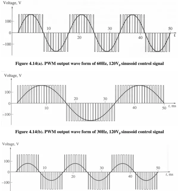
A dolgozatban bemutatásra kerülnek a jelenleg iparilag használt fordulatszám érzékelő nélküli szabályozást biztosító megoldások, mint a referencia motormodellek, adaptív megfigyelők, MRAS, DTC, és vektor alapú technikák, melyek összehasonlításra kerülnek az általunk adott szabályzási struktúrával. Ezenkívül, a mai aszinkronmotoros hajtások elvi és gyakorlati felépítését is megvizsgáljuk a gerjesztés előállítására szolgáló impulzus szélesség modulációs (PWM) technikák bemutatása mellet.
Az implementáció alapjául szolgáló mikrokontroller vezérelt térvektor (SV)-PWM VSI betáplálású hajtásláncot részletesen elemezzük az általunk tervezett szabályzó megvalósítási lehetőségeinek függvényében, és az implementáció által a Code Composer fejlesztői környezetben létrehozott ANSI C programot valamint a hajtásban felhasznált aszinkronmotor paraméter identifikációját is ismertetjük. A dolgozatot a mérések és a szimulációk alapján kapott eredmények vizsgálata zárja a hajtás jóságára, hatékonyságára, robusztusságának és stabilitására vonatkozó következtetések és a továbbfejlesztési lehetőségek ismertetése mellett.
The thesis shows the implementation of a robust control structure for the speed sensorless vector control of the induction motor (IM) on a TMS320F243 processor controlled voltage source inverter (VSI) driven laboratory induction motor drive.
The designed robust controller whose design is based on the modern achievements of Control and Systems theory (such as the politopic system representation based H∞ controller and observer synthesis, the mixed sensitivity structures, small gain theorem, and the theory of extended Kalman filters (EKF)) is presented which makes possible the direct control of the flux and speed on the full 4/4 operation range of the motor with torque adaptation in highly noisy industrial environment. In this way the produced structure fulfills the recently growing expectations for industrial drives as the control without speed sensors (with the measurements only of the phase currents), robust stability, and noise attenuation. The designed closed loop control system is tested by intensive Matlab/Simulink simulations that are presented in the thesis to prove the goodness of the solution, which according to the results shows good dynamic and robust performance.
In this paper the recently used speed sensorless techniques in the industry, such as the direct reference models, adaptive observers, MRAS, DTC, and vector control based methods are shown and compared to the designed controller structure. Moreover, the theoretical and practical concepts of the modern IM drives and the pulse width modulation (PWM) based the power feed generation methods of these devices are also presented.
The microcontroller driven space vector (SV)-PWM VSI fed drive, which is used for the implementation of the controller, is analyzed in details with respect to the concepts of the controller realization. The implementation resulted ANSI C program in the Code Composer development environment is also explained with the parameter identification of the applied motor of the laboratory drive. The experienced measurement and simulation outcomes of the implementation are evaluated in terms of effectiveness, robustness, and stability and the obtained conclusions are drawn. Finally, possible improvements of the control structure and future applications are pointed out as well.
Key words: induction motor, H∞,LPV,EKF, mixed sensitivity, speed sensorless control, TMS320F243 EVM, DTC, MRAS, vector control, SV-PWM
Table of contents
Abbreviations... vi
1. Introduction... 1
2. The mathematical model of the induction motor... 4
2.1. Basic concepts of operation ... 4
2.2. Modeling conditions ... 6
2.3. General mathematical description ... 6
2.3.1. Voltage and flux equations ... 9
2.3.2. The dynamical motion equation ... 11
2.3.3. Approximation of rotor resistance variation... 12
2.4. Model representation in rotating reference frame ... 13
2.4.1. General reference orientation ... 15
2.4.2. Rotor flux oriented representation ... 16
2.5. The linear parameter variant motor model ... 17
2.6. General dynamic properties of the model... 20
3. Existing speed sensorless techniques... 22
3.1. Constant Volts per Hertz control ... 22
3.2. Machine models... 26
3.2.1. Direct reference models ... 27
3.3. Adaptive observers & filters ... 29
3.3.1. Full order nonlinear observer... 29
3.3.2. Sliding mode observer ... 31
3.3.3. Extended Kalman Filter ... 32
3.3.4. H∞ based LPV observer ... 34
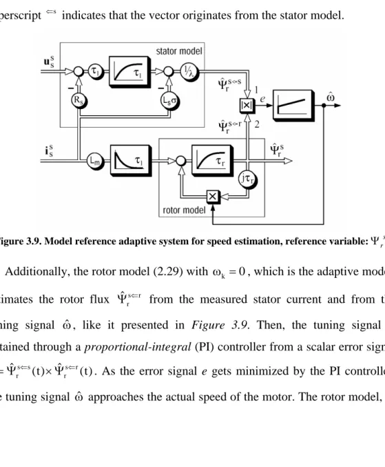
3.3.5. Model reference adaptive systems... 36
3.4. Direct torque control... 38
3.5. Vector control ... 44
3.6. Fuzzy control ... 46
4. Operation of induction motor drives... 49
4.1. Classical power feed generation concepts ... 49
4.1.1. Rectifier ... 50
4.1.2. DC link... 52
4.1.3. Inverters ... 52
4.1.4. Inverter control circuitry... 53
4.1.5. The microcontroller ... 54
4.2. The PWM inverters... 54
4.2.2. The mechanism of PWM-VSI inverters ... 55
4.2.3. Different techniques of the 3-phase PWM generation on VSI-PWM inverters ... 62 4.2.3.1. Synchronous symmetric PWM ... 62 4.2.3.2. Synchronous asymmetric PWM ... 62 4.2.3.3. Asynchronous PWM... 62 4.2.3.4. Space vector PWM ... 63 4.2.3.5. Overmodulated PWM... 65
5. The experimental laboratory drive... 67
5.1. The induction motor ... 68
5.2. The Spectrum Digital inverter ... 70
5.2.1. Specifications of the inverter module ... 70
5.2.2. Capabilities of the inverter module ... 71
5.2.3. Sensors ... 72
5.2.4. Built in protections ... 73
5.3. The Inverter Interface Card ... 73
5.3.1. Specifications of the interface module ... 74
5.3.2. I/O signal conditioning ... 74
5.3.3. Inverter Digital Interface ... 75
5.3.4. Shield of the drive... 76
5.4. The TMS320F243 Evaluation Module... 76
5.4.1. Specifications of the EVM... 77
5.4.2. Considerations of controller implementation ... 78
5.4.3. Chip of many things... 78
5.4.3.1. Speed and memory ... 79
5.4.3.2. Interrupts and peripherals ... 80
5.4.3.3. Digital I/O pins ... 82
5.4.3.4. Event manager (EVM2)... 82
5.4.3.4.1. Timers ... 82
5.4.3.4.2. PWM generation ... 84
5.4.3.4.3. Deadband unit ... 87
5.4.3.4.4. Capture units ... 87
5.4.3.4.5. Quadrature Encoder Pulse (QEP) Circuit... 88
5.4.3.4.6. Analog to digital converter (ADC) ... 89
5.4.3.5. Communication interface... 90
5.4.3.5.1. Serial Communications Interface (SCI) ... 90
5.4.3.5.2. Serial Peripheral Interface (SPI)... 91
5.4.3.5.3. Controller are network interface (CAN)... 91
5.4.4. Heart and soul of the drive... 92
5.5. The PC ... 93
5.5.1. The XMS510P Plus JTAG driver ... 93
5.5.2. The Code Composer environment ... 93
5.5.3. The operator interface... 94
6. Implementation of the controller ... 95
6.1. The theoretical structure of control... 96
6.1.1. The H∞ controller module... 98
6.1.2. I/O linearization based reference transformation ... 99
6.1.3. Rotor flux orientation and flux angle tracking ... 101
6.1.4. The structure of estimation ... 102
6.1.5. The H∞ observer... 103
6.1.6. The EKF... 104
6.1.7. Estimation of the load torque... 106
6.1.8. Tuning parameters ... 106
6.2. Simulation results ... 107
6.3. The identification of the motor ... 114
6.3.1. Method of identification ... 115
6.3.2. Measurements ... 118
6.3.3. Results of the identification ... 120
6.3.4. Validation of the model ... 121
6.4. The program of the DSP ... 121
6.4.1. Flow chart of the program ... 122
6.4.2. The hardware boot up ... 123
6.4.3. System initialization and hardwired constants ... 124
6.4.4. Control loop ... 125 6.4.5. Process of ADC ... 125 6.4.6. Processes of estimation... 127 6.4.7. Process of control ... 128 6.4.8. Process of PWM generation ... 128 6.4.9. Additional features... 129 6.5. Speed considerations ... 129 7. Conclusion ... 132 References... 134
Table of notations
n(t) rotor speed [revolution/sec] Rsx stator side resistance of phase x [Ω] 0
n synchronous frequency [Hz] Rs stator side 3 phase resistance [Ω] 0
f input synchronous frequency [Hz] Rr rotor side 3 phase resistance [Ω]
p number of pole pairs R0 initial value of Rr[Ω]
ω(t) angular speed of the rotor [rad/sec] Ls lumped stator 3 phase induc. [H] 0
ω sync. angular speed [rad/sec] Lr lumped rotor 3 phase induc. [H]
k(t)
ω angular speed of rotating reference
frame [rad/sec] Lm lumped mutual 3 phase induc. [H] rflux(t)
ω ang. speed of rotor flux [rad/sec] ls stator winding phase inductivity [H]
ref(t)
ω ref. signal of rotor speed [rad/sec] lr rotor winding phase inductivity [H]
s(t) slip lf field inductivity [H] sx
F ( , t)α current density distribution in phase
x [A/rad] lm mutual inductivity [H] sx
i (t) stator current in phase x [A] C capacity [F]
sx
u (t) stator voltage in phase x [V] ρ(t) angle between the stator fixed and the rotor fixed reference frame [rad]
Ψ magnetic flux [Wb] ρk(t)
angle between the stator fixed and the rotating reference frame [rad]
i
ϕ init. ang. of stat. current vec. [rad] Pmech(t) mechanical power [W]
u
ϕ init. ang. of stat. voltage vec. [rad] Wmech(t) mechanical energy [J]
a three-phase unity vector W (t)e electrical input power [J] s
x space vector in stat. fixed rep. W (t)v resistive power loss [J] r
x space vector in rotor fixed rep. Wfield(t) air gap power of magnetic field [J] fr
x space vect. in rotor field orient. rep. Te(t) electromagnetic torque [Nm] k
x space vect. in rotating ref. frame Tload(t) load torque [Nm]
d
x real part of space vector x in
rotating reference frame τmech mechanical time constant [Nm] q
x imaginary part of space vector x in
rotating reference frame τe electrical time constant [Nm]
xα real part of space vector x in stator
fixed reference frame τs stator time constant (constant)
xβ imaginary part of space vector x in
stator fixed refernce frame τr rotor time constant (constant) nominal
x nominal value of signal x τ m. coupling time constant (constant)
ref
x reference signal of x σ leakage factor (constant)
error
x error signal of x λ notation, def. pp. (constant)
x sa(t)
i space vector describing current
density distribution of phase x [A] J moment of inertia [Nm]
x s(t)
i space vector describing the overall
stator side cur. density distrib. [A] T(t) rotor temperature [K]
x
(t)
x s (t)
Ψ space vec. describing the overall
stator side flux linkage distrib. [Wb] Q(t) heat [kcal]
x r (t)
Ψ space vec. describing the overall
rotor side flux linkage distrib. [Wb] c specific heat ct. Al [J/kgK]
x
(t)
σ
Ψ space vec. describing the overall
leakage flux distrib. [Wb] m weight of the rotor winding [kg]
x s(t)
u space vector describing the overall
stator side volt. density distrib. [V] Kk linear heat convection (constant) x
r(t)
u space vector describing the overall
rotor side volt. density distrib. [V] F fraction (constant)
r eff
i (t) rms value of the rotor phase cur. [A] h discrete time step [sec]
s eff
i (t) rms value of the stator p. cur. [A] t time [sec]
s eff
u (t) rms value of the stator p. volt. [V] ν,α angle [rad]
sp
i (t) active stator current [A] K contr. of general problem definition Ubus inverter bus voltage P
considered system (plant) of the general problem definition
x
u xth switching state of the inverter p parameter vector
x or x 60 ±
u voltage vect. of sector x (SV-PWM) x state vector of the system
in
u (t) control voltage of the PWM G(s) frequency transition func. of the sys.
x ,y
u (t) x or y ref. voltage of the PWM x(k k) estimated state vector based on k
pervious estimations
out
u (t) output voltage of the PWM P(k k) covariance of the error process
out 0
U amplitude of the fundamental
frequency component x error of the estimation mFM frequency modulation value y output vector of the system
mAM amplitude modulation value u control/general system input
Vp peak voltage value v vector of measured output signals
Vpp peak to peak voltage value z system output vector (optimization)
x( )ωˆ
S complex gain factor w input disturbances of the system
f(x,u) state function (non linear state space
sys. description ) e error signals of the system
f(x) state func. of an input-affine model R covariance of measurement noises
fd(x) discretised state function Q covariance of system noises
h(x) output function (non linear state
space sys. description ) γ optimal H∞gain
hd(x) discretised output function v1, v2 virtual inputs
g(u) input func. of an input-affine model xˆ predicted / normalized value
gd(u) discretised input function δ scaling step size/Re. of comp. freq.
Ξ sequence of measured values T1, T2 Modulation times in the SV-PWM
θ parameter values αu angle of stator voltage vec. [rad]
(.)
G first order gradient vector ∆ change / error of a given variable
2(.)
G second order gradient vector λfilter gain of the exponential filter
Abbreviations
AC Analog Current/Voltage MIPS Million Instructions Per Second ACG Automated Code Generation MOSFET Metal Oxide Semiconductor Field
Effect Transistor
AI Artificial Intelligence MRAS Model Reference Adaptive Control
AS Asymmetric Synchronous NL Nonlinear (system) CAN Controller Area Network NMI Non Maskable Interrupt
CPU Central Processing Unit NRZ Non Return to Zero DC Direct Current/Voltage PC Personal Computer
DSP Digital Signal Processor PIC Programmable Integrated Circuit DTC Direct Torque Control PID Proportional, Integrational,
Derivational (control) EC External Commutation PWM Pulse Width Modulation EKF Extended Kalman Filter QEP Quadrature Encoder Pulse EVM Evaluation Module RAM Random-Access Memory EVM2 Event Manager ROM Read-Only Memory
FIFO First In First Out (data storage) RTDX Real-Time Data Exchange FLC Fuzzy Logic Control SC Self Commutation
GEL General Extension Language SCI Serial Communication Interface GP General Purpose SPI Serial Peripheral Interface IDE Integrated Development
Environment
SS Symmetric Synchronous
IGBT Isolated Gate Bipolar Transistor SV-PWM Space Vector based Pulse Width Modulation
JTAG Joint Test Action Group (IEEE 1149.1)
TI Texas Instruments
LPV Linear Parameter Variant (system)
UART Universal Asynchronous Receiver/Transmitter LQG Linear Quadratic Gaussian
Control
UML Unified Modeling Language
LTI Linear Time Invariant (system) VSI Voltage Source Inverter LTV Linear Time Variant (system) WD Watch Dog
1.
Introduction
Induction motors are widely used in the industry due to their simple structure, low cost, and high reliability. Although they have become dominant only in the past decades on the field of variable speed electrical drives, their economical importance is noteworthy with more than 12 billion US$ world market volume, of which the annual growth rate is 15%. [18]
The construction of the first induction motor (IM) was a significant breakthrough in the field of electrical machines. In 1888, Tesla received half a million dollars from the Westinghouse for the patent of his invention. Unfortunately, this was followed by 60 years of banishment, because it quickly turned out that the control of this electrical machine is a challenging task [31]. Difficulties had risen because of its highly nonlinear nature and the low technology level of Power Electronics. The nonlinear dynamic behavior of this system, which is even effected by parameter disturbances, prevented the effective use of the analog control methods. Moreover, the extremely important strength and orientation of the magnetic field, described by the magnetic flux (Ψ), can be only expensively and inaccurately measured, so its control needs mathematical estimation. Furthermore, some of the parameters of the IMs, like the variation of the rotor resistance (Rr), introduce large uncertainties into the system behavior.
These were the reasons for the golden age of DC motors which provide easy controllability and power management with a more complicated construction [19]. By the improvement of technology, like the evolution of control and system theories and the important results in Power Electronics, as the isolated gate
bibolar transistor (IGBT) and the cheap, reliable, and high frequency inverters,
the induction drives have slowly overtaken this field and become the horsepower of the industry, providing more than 90% of today’s industrial drives. The success of the IMs can be explained by their simple structure and the need of less maintenance because of the absence of graphite brushes.
Only in those fields which need simple control and high precision preserved the DC motors their leading role. Nowadays, therefore, there is a great interest in
developing high performance and robust controllers to make induction drives unbeatable in all fields of applications. Especially, these efforts concentrate on controllers that do not need speed sensors to operate, which greatly reduces costs and maintenance. Modern industrial drives also need to be insensitive for the heavy noises of the industrial environment and be able to adapt to parameter uncertainties related to manufacturing.
Motivated by this goal and based on modern mathematical methods and physical considerations, we show the implementation of a robust, speed sensorless controller on a TMS320F243 digital signal processor (DSP) controlled induction motor drive that gives the opportunity of fast control of the motor speed and the magnetic field associated with the rotor flux (Ψr = [Ψrα, Ψrβ]T) on the full 4/4
operation range of the motor. The voltage feed of the IM is generated by a voltage
source inverter (VSI), which is connected with an interface card to the DSP. The
full operation of the drive is shown with the steps of the implementation of the obtained controller. Moreover, as the result of the implementation, the produced DSP program with its unique methods is presented in C as well. According to the theoretical and practical results, this realization holds the possibility of good performance and fulfills the needs of the modern industrial expectations.
To be able to explain the solution of the considered control problem, firstly the dynamic mathematical model of the IM is introduced with the self constructed
linear parameter variant (LPV) system model of the motor. Then, the main
dynamic properties of the given models are analyzed.
In the next section the existing speed sensorless techniques are presented briefly to provide good look out to the most up-to-date techniques used in sensorless IM drives. The usage and effectiveness of the showed methods are analyzed and their disadvantages and applicabilities are pointed out.
In the third section the problem is investigated from the point of view of power systems. The existing techniques to provide the power feed of the drive are presented with the mechanism of the inverters.
Then the self-assembled laboratory drive is focused on, with the description of the physical layout and by the introduction of each hardware element of the drive.
Several issues of implementation are analyzed and the specification of an applicable control structure is given.
In the sixth section the implemented control algorithm is introduced and investigated from both theoretical and practical aspects. The results of the numerically simulated performance are presented in the case of intensive and dynamic changes of the operation environment to prove the effectiveness of the algorithm. The nonlinear parameter identification of the motor model is also analyzed, based on the results of measurements and on the theory of the gradient method. Furthermore, the self-written DSP program, which makes possible the implementation of the presented algorithm in C is also given and analyzed in the point of view of optimality.
Finally, the results of the implemented drive are given and compared with other published results in this field. Furthermore, at the end, the further possibilities of improvements of the system are considered with the ongoing research efforts.
2.
The mathematical model of the induction motor
2.1.
Basic concepts of operation
In the the following section, the structure of the induction motors and their main features of functioning are introduced based on [6, 12, 20, 21, 26, 32].
The structure of the IMs can be divided into two parts, namely the stator and the rotor, as it can be seen in Figure 2.1. The stator, which is built up from good flux conducting plates, is held together by a cast-iron hull. In the other part, the voltage powered stator winding is situated in the shaft-oriented rabbets on the inner side cylinder of the plated motor hull. This stator winding is usually mathematically modeled by an infinitely fine coil continuously wrapped around the inner side cylinder of the stator. The three-phase AC voltage, which is applied to this winding, serves as the power source of electrical torque that produces the mechanical motion. The other part, which is called the rotor, has mechanical connection only through bearings with the stator and it is crafted from iron plates. The three-phase winding of the rotor is situated in similar rabbets around the surface like the stator winding. In those motors of which the rated power is less then 10kW, these rotor coils are usually built from aluminum bars, which are connected by conducting rings on the front side of the plated body. This type of design is called squirrel-cage motor and it is very typical in most of the applications of the IM. In the following section, this type of the IM is considered.
In Figure 2.1, the schematics of the motor can be seen, where an air gap separates the previously mentioned stator and rotor parts. The existence of this air gap is important, because through it, the rotor is connected only magnetically to the stator. Based on this, the two parts can be modeled by the primer and secunder sides of a rotating transformator which is described by complex quantities due to the rotation. Similarly to the properties of a transformator, the magnetic coupling through the air gap provides the flow of energy between the two electrical subsystems, and therefore has a significant role in the overall efficiency of the IM.
The mechanism of the motor is briefly the following: when three-phase AC voltage is applied to the evenly distributed coils around the cylinder of the stator, a rotating magnetic field is built up inside the machine, which produces sinusoidal current inside the rotor winding based on the induction phenomena. This inducted current also produces a rotating magnetic field around the rotor which tries to extinct the effect that brought it to existence. Thus, it tries to line up to the magnetic field of the stator in strength and in orientation as well, but because of the field of the stator rotates and the induction in the rotor lessens when the two magnetic fields approach closer, the field of the rotor can never align with the field of the stator. After the transients an equilibrium state is reached when the two fields rotate with the same speed, which is called synchronous frequency, but the field of the rotor always lags behind the field of the stator. Moreover, the interaction between the two magnetic fields produces a electromagnetic force
(emf), whose effect is orthogonal to the shaft and forces the rotor to rotate. The speed of the rotor is noted by n(t), which is usually given in angular speed:
(t) 2 n(t)
ω = π⋅ , and the synchronous speed of the magnetic field can be described as follows:
0 0
f input frequency
n ,
p number of pole pairs
= = (2.1)
which is usually given in angular frequency: ω = π0 2 n0. Furthermore, the normalized difference of the two speed is the slip (s) of the motor:
0 0 n n s . n − = (2.2)
The slip is directly related to the load torque and it describes the equilibrium state of the electromagnetical interaction. s(t)∈
(
0,1]
(in motoric operation range) Based on the direction of the energy flow, the IM can be operated as a motor and a generator as well, although it is barely used as a generator because of efficiency related issues. In this paper, only the motoric operation of the IM is going to be described.2.2.
Modeling conditions
In the next sections, the squirrel-cage type IM is considered whose physical layout parameters are already included in the synchron frequency of the magnetic field and in the mechanical time constant of the machine. Beside this, the following assumptions are made, which are widely common in mathematical investigations of this physical phenomena [32]:
The permeability of the iron body of the rotor is assumed to be infinite with linear magnetic properties, so the saturation phenomena do not affect the magnetic coupling.
The iron core is assumed to be homogeneous, thus circular parasite currents are not produced inside the core which would lessen the induction. Slotting effects, like deep bar and end effects are also neglected.
The spatial distribution of the phase currents in the stator winding is considered to be sinusoidal, which describes two half moons shape density distribution rotating along the cylinder of the stator.
The three-phase star connection of the stator coils has symmetric electrical parameters, and the input excitation is also a perfectly symmetric three-phase voltage or current feed.
2.3.
General mathematical description
By applying the above mentioned assumptions and neglecting the described loss effects to the description of the motor, the instantaneous spatial distribution of one phase current can be given as Figure 2.2. In the following, the mathematical description of the motor is investigated through the space vector
theory introduced in [26] to be able to use the possibilities provided by this approach. If it is assumed that the current of the stator is the input excitation of the machine, than the F ( , t)sx α spatial distribution along the stator of the x phase current can be described by the issx(t) complex vector whose orientation is determined by the direction of the respective phase axis and the current polarity [18]. In the presented case the positive phase current issa(t) in stator winding phase a creates a sinusoidal current density distribution that leads the winding axis
a by 90°, having therefore its maximum in the direction of the imaginary axis.
Figure 2.2. Current density Figure 2.3. Stator side current distribution of phase a density distribution
The total magnetomotoric force (mmf.) inside the motor is obtained as the superposition of the current density distributions of all three phases. This produces again a sinusoidal distribution of the overall stator current density wave indicated
by Figure 2.3. The iss(t) space vector, which describes this overall current
distribution, can be given by the superposition of the space vectors of each phase as it can be seen in Figure 2.3. Furthermore, iss(t) can be also computed from the positive successive representation of the symmetric phase currents:
0 i sa sb sc j t s 0 2 s 2 s sa sb sc eff ( t ) ( t ) ( t ) 2 (t) i (t) i (t) i (t) 2 i (t) e , 3 π ω + +ϕ = ⋅ + ⋅ + ⋅ = ⋅ ⋅ i i i i a a a (2.3)
{ }
s{
2 s}
{
s}
sa s sb s sc s i (t)=Re i (t) , i (t)=Re a ⋅i (t) , i (t)=Re a i⋅ (t) , (2.4)where 2 j 3 e π =
a is the complex unity vector that describes the phase lags and the space orientation of the current density distributions to each other along the stator. For completeness, equation (2.4) provides the inverse transformation of (2.3). So
s(t)
i , the stator current space vector, represents the sinusoidal spatial distribution of the total mmf. wave created inside the machine by the three phase currents that flow from the outside of the machine. The mmf. wave has its maximum in an angular position that leads is(t) by 90° as illustrated in Figure 2.3. The amplitude of this mmf. is proportional to is(t) . Furthermore, the scaling factor 2/3 presented in the equation (2.3) reflects the fact that the total density distribution is obtained as the superposition of the density distributions of the three phase windings, while the contribution of only two phase windings, spaced 90° apart, would have the same spatial effect with the phase currents properly adjusted. Therefore, it provides the scaling factor from three-phase description to the two-phase based complex representation. This approach is called energy invariant representation and it is used in the following to construct the model of the IM.
The excitation produced flux density distribution in the air gap is obtained by spatial integration of the current density wave along the cylinder of the stator. Therefore, it is also a sinusoidal wave, and it lags the current density wave by 90° as illustrated in Figure 2.4.
Figure 2.4. Stator side overall flux linkage distribution
It is convenient to choose the flux linkage wave, as a system variable instead of the flux density wave as the former contains added information on the winding
geometry and the number of turns of the coil. By definition, a flux linkage distribution has the same spatial orientation as the pertaining flux density distribution, therefore the stator flux linkage distribution presented in Figure 2.4
can be described by the space vector Ψss(t). Based on same reasons, the Ψrr(t) space vector can be also introduced to represent the rotor flux linkage distribution. In the individual stator windings, the rotating flux density wave induces voltages. Since the winding densities are sinusoidal spatial functions, therefore the induced voltages are also sinusoidally distributed in space. The same is true for the resistive voltage drop in the windings. Thus, the overall distributed voltages in all phase windings can be represented by the uss(t) stator voltage space vector, which is a complex variable and can also be computed from the positive successive representation of the stator phase voltages:
0 u sa sb sc j t s 0 2 s 2 s sa sb sc eff ( t ) ( t ) ( t ) 2 (t) u (t) u (t) u (t) 2 u (t) e , 3 π ω + +ϕ = ⋅ + ⋅ + ⋅ = ⋅ ⋅ u u u u a a a (2.5)
{ }
s{
2 s}
{
s}
sa s sb s sc s u (t)=Re u (t) , u (t)=Re a u⋅ (t) , u (t)=Re a u⋅ (t) . (2.6)2.3.1. Voltage and flux equations
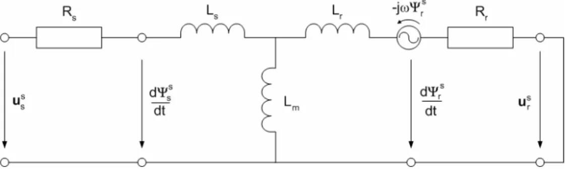
If we consider the primer side of the complex transformator (Figure 2.5) as the stator of the IM, then equation (2.7) describes the connection between the introduced stator side space vectors:
s s s s s s s d (t) (t) (t) R , dt = ⋅ + u i Ψ (2.7)
where iss(t) R⋅ s is the resistive voltage drop and Rs =Rsa =Rsb =Rsc denotes the resistance of the symmetric stator phase windings. The induced voltage vector, represented by the last term of (2.7), is the back electromagnetic force (emf.).
Figure 2.5. Complex transformator that describes the model of the IM
By considering the secunder side of the complex transformator, it can be concluded that the same relationship is true to the rotor side space vectors, but because of the short circuited rotor winding, in this case urr(t)=0, t∀ ∈ , thus
r r r r r r r d (t) (t) (t) R . dt = ⋅ + = u i Ψ 0 (2.8)
Equation (2.7) and (2.8) describe the electromagnetic interaction as the connection of first order dynamic subsystems. Because four complex variables:
s r s r
s(t), r(t), (t), (t)s r
i i Ψ Ψ are presented in these two equations, (2.9) and (2.10) flux equations are needed to complete the relationship between them.
s s r j ( t ) s(t) s(t) Ls r(t) Lm e ρ =i ⋅ +i ⋅ ⋅ Ψ , (2.9) r s j ( t ) r r(t) s(t) Lm e r(t) Lr − ρ =i ⋅ ⋅ +i ⋅ Ψ , (2.10)
where the presented (t)ρ angle describes the position of the rotor compared to the axis of the stator, while 3 3
2 2
r r f
L = l + l , 3 3
2 2
s s f
L = l + l are the three-phase inductances and l , l are the inductances of a stator and a rotor phase winding, s r
f
l is the self inductance, and 3 2
m m
L = l is the mutual inductance between the stator and the rotor [32]. In order to eliminate the (t)ρ angle from the model equations transformation of rotor side vectors into the reference frame of the stator is needed. Thus, by applying the following substitutions: isr(t)=irr(t) e⋅ j ( t )ρ and
s r j ( t )
r(t) r(t) e
ρ
= ⋅
s s s s(t)=is(t) L⋅ s+ir(t) L⋅ m Ψ (2.11) s s s r(t)=is(t) L⋅ m +ir(t) L⋅ r Ψ (2.12)
equations provides the flux connections in the model, while, because of the consistence of the transformations, (2.7) and (2.8) do not change.
2.3.2. The dynamical motion equation
Based on the concept of energy considerations, the electromagnetic torque of the motor can be derived easily [26]. For the mechanic power Pmech(t) of the system, the following is true:
mech mech dW (t) P (t) , dt = (2.13)
where the mechanical energy Wmech(t) in case of rotating systems can be given by
mech
e
dW (t)
T (t) (t).
dt = ⋅ω (2.14)
However, it is also true that the mechanical energy can be presented in the form of
e mech v field W (t)=W (t)+W (t)+W (t), (2.15) where
{
}
s s* s s* e s s r r dW (t) 3 Re ,dt = 2 u i⋅ + ⋅u i is the input electric power,
{
}
2 2 s r v s s r r dW (t) 3 Re R R ,dt = 2 i + i is the resistive power loss, s s s* s* field s r s r dW (t) 3 d d Re , dt 2 dt dt = + i i Ψ Ψ
is the air gap power.
Here, the complex conjugation was noted by *. By substituting the above equations into (2.14), it can be concluded that:
s s m mech e r s r L 3 P T (t) (t). 2 L = ⋅ω = ωΨ ×i (2.16)
From (2.16) the electromagnetic torque of the motor can be expressed in case of a p polyphase machine: s s m e r s r L 3 T (t) p (t) (t). 2 L = Ψ ×i (2.17)
It must be noted that (2.17) can also be given as a product of any two of the
s r s r
s(t), r(t), (t), (t)s r
i i Ψ Ψ state variables by appropriate scaling. Furthermore, for the mechanical subsystem of the motor, the dynamical motion equation is as follows: mech e load d (t) T T F (t), dt ω τ = − − ω (2.18)
where τmech =J / p is the mechanical time constant, J is the moment of inertia, load
T is the load torque, and F (t)ω is the energy loss due to friction. Based on (2.18), the differential equation, describing the change of ω, the angular speed of the rotor, can be derived as follows:
(
)
e 2 s s load m r s r mech 1/ T (t) F (t) 3p L d (t) (t) (t) . dt 2JL τ + ω ω = ⋅ × − τ i Ψ (2.19)2.3.3. Approximation of rotor resistance variation
Because the parameter uncertainties have great impact on the overall system dynamics, the most significant rotor resistance variation has to be modeled somehow for an accurate description of the system. However, it is not rewarding to give very detailed description of this change, because the value of R is unique r for every IM and its dynamic properties strongly depend on the layout and the built-in materials of the motor and on other uncertain parameters [40]. Thus, only an approximation of the real description is needed to model the most important dynamics of the uncertain parameter variations. It is known that the resistance change to heat of a given aluminum body with linear heating characteristics is as follows: r 0 0 R (t) R R , T(t) T 245 T − = − + (2.20)
where R is the rotor resistance at 0 T normal temperature, and 245 is the specific 0 constant of the aluminum. Furthermore, the heat produced by the electrical energy can be given by (2.21).
(
)
0 t 2 r eff r t Q(t)=0.86⋅∫
i (t) ⋅R (t)dt. (2.21) By considering the heating properties of materials:0
Q(t)= ⋅ ⋅m c (T(t) T ),− (2.22)
is also true, where c is the specific heat, m is the weight of the aluminum bars. Based on equations (2.20), (2.21), and (2.22) it can be concluded that
(
)
(
)
(
)
T 0 2 r 0 r eff k r 0 0 R 0.86 R dR (t) i (t) R(t) K R (t) R , dt 245 T m c ⋅ = ⋅ ⋅ − − + ⋅ ⋅ (2.23)if it is assumed, that the heat dissipation to the environment depends only on the energy leaking caused by convection, which is linear and it is described by the rate constant K . k
2.4.
Model representation in rotating reference frame
The representation of the motor model in a rotating reference frame, introduced by Blaschke, Hasse, and Leonard more than 20 years ago, has completely changed the field of controller synthetisation for asynchronous motors [41]. They formed the basic idea of the space vector based direct torque control, which has been recently the most widely used method for IM drives. This basic idea is the following: introduce such a new coordinate system, which rotates with ωk angular speed against the previously used stator fixed reference frame.
On this way, at any time instant, if the angle between the real stator axis and the real axis of the new reference frame is ρk, then the flux space vectors in this representation (see Figure 2.6) can be given in the following form:
Figure 2.6. Rotating two-phase coordinate system
(
)
k k k j ( t ) k s k s j ( t ) k j ( t ) s s k s d (t) e d (t) d (t) d (t) e j (t) e dt dt dt dt ρ ρ ρ ⋅ ρ = Ψ = ⋅ + ⋅ ⋅ Ψ Ψ Ψ (2.24) ( )(
)
( ) ( ) k k k j ( t ) ( t ) k r r r k j ( t ) ( t ) k j ( t ) ( t ) r k r d (t) e d (t) dt dt d (t) d (t) d (t) e j (t) e dt dt dt ρ −ρ ρ −ρ ρ −ρ ⋅ = = ρ ρ = ⋅ + − ⋅ ⋅ Ψ Ψ Ψ Ψ (2.25)where the vectors presented with index k are the transformed vectors of the rotating reference frame, k
k d (t)
(t) dt
ρ
= ω is the angular speed of the reference rotation, and d (t) (t)
dt ρ
= ω is the angular speed of the rotor. By applying the reference transformation to all of the space vectors, equation (2.7) and (2.8) are reformed as follows: k k k s j ( t ) j ( t ) j ( t ) k s s s s s s s k k s k s s k s d (t) (t) (t) e (t) e R e dt d (t) (t) R j (t) . dt − ρ − ρ − ρ = ⋅ = ⋅ ⋅ + ⋅ = = ⋅ + + ω u u i i Ψ Ψ Ψ (2.26) ( ) ( ) ( )
(
)
k k k r j ( t ) ( t ) j ( t ) ( t ) j ( t ) ( t ) k r r r r r r r k k r k r r k r d (t) 0 (t) (t) e (t) e R e dt d (t) (t) R j (t) . dt − ρ −ρ − ρ −ρ − ρ −ρ = = ⋅ = ⋅ ⋅ + ⋅ = ⋅ + + ω − ω u u i i Ψ Ψ Ψ (2.27)By the consistency of the transformation, (2.11) and (2.12) preserve their original forms.
2.4.1. General reference orientation
Let equations (2.11), (2.12), (2.26), and (2.27) are considered in a general reference frame rotating with the angular speed of ωk. In this case, any two of the
k k k k
s(t), r(t), (t), (t)s r
i i Ψ Ψ space vectors can be chosen to state variable during the formulation of the model, but for decoupled control of the flux and speed, it is worth choosing isk(t) and Ψrk(t) for the states of the system. On this way, from (2.11) and (2.12): 2 k s r m k m k s s r r r L L L L (t) (t) (t), L L − = ⋅i + ⋅ Ψ Ψ (2.28)
can be formulated with
(
)
k k k r m r r s k r r r d (t) L R R (t) j (t), dt L L = − + ω − ω i Ψ Ψ (2.29) from (2.27) and 2 k 2 2 k k s r m s m s r m s 2 r s k s r r r k m r m r 2 r r L L L d (t) L L L L (t) R R j (t) L dt L L L R L j (t), L L − ⋅ = − + + ω ⋅ − ⋅ + − ω⋅ ⋅ i u i Ψ (2.30)from (2.26). Also, the exact state equation can be derived from (2.29) and (2.30). If we decompose our complex variables to their real (d) and imaginary (q) parts, and suppose that the rotor resistance varies, then the following input-affine state space equations system, which is nonlinear in ω ω, k, and Rr, describes the model.
( ) ( ) k r m k r r k rd m k k r r rq k sd r s k k r sq r s k r ( , ,R ) L 1 (t) 0 (t) (t) (t) 1 L (t) 0 (t) (t) (t) d i (t) ( (t) ) dt (t) (t) i (t) ( (t) ) (t) (t) ω ω − ω − ω τ τ Ψ − ω − ω − Ψ τ τ = τ ω ⋅τ − λτ + τ ω σ⋅ τ σ σ −ω ⋅τ τ −ω − λτ + τ σ σ⋅ τ σ A k rd k k rq sd k k s sd sq k sq s 0 0 (t) 0 0 (t) 1 u (t) 0 L i (t) u (t) i (t) 1 0 L Ψ Ψ ⋅ + σ ⋅ σ B (2.31)
where σ = 1 – (Lm)2 / (Ls · Lr), λ = (Lm)2 / Ls, τ = Lm / (Ls · Lr), τr(t)= Lr / Rr(t), τs = Ls / Rs. Besides (2.31) the k k k k rd sq rq sd load e mech (t) i (t) (t) i (t) T (t) F (t) d (t) , dt Ψ ⋅ − Ψ ⋅ + ω ω = − τ τ (2.32)
motion and the
(
)
2 2 k k k k rq m sq rd m sd r T0 k r 0 r r (t) L i (t) (t) L i (t) dR (t) R R(t) K R (t) R , dt L L Ψ − Ψ − = ⋅ + ⋅ − − (2.33)rotor resistance nonlinear differential equations complete the description of the system by defining the variance of the parameters of the state matrix
k r
( ,ω ω , R )
A , from which ω and R are representation independent parameters r of the (2.31) motor model, while ωk defines the representation of the model. If
k 0,
ω = then the real part of the state variables is indexed with α and the imaginary part is with β.
2.4.2. Rotor flux oriented representation
Nowadays, there are several representations of the motor model used in the field of IM drives, based on the value chosen for ωk. From these possible representations, only the field oriented approach is considered in the following section, because as it is going to be shown, this orientation makes possible the design of an efficient controller with ease. By this approach, a new reference frame is introduced, where the real axis is bounded to the rotating Ψrk(t) vector, thus ω = ωk rflux. In this case, k
r (t)
Ψ has no imaginary component, which fact implies the reducement of the state variables by letting out Ψrqk(t) from the model. Moreover, because at steady state all of the stator side electrical quantities
(Figure 2.7) in the stator fixed reference frame rotate with the same synchronous
frequency of the flux fields, these field-orientated variables are constants. So in this way, ωrflux = ω0, and (2.31) is transformed into the following form:
Figure 2.7. Rotor field orientation in two phase rotating reference frame m fr r r fr rd rd fr sd fr r s fr sd rflux sd r s fr fr sq sq r s rflux s L 1 0 (t) (t) 0 0 (t) (t) u ( (t) ) d 1 i (t) i (t) 0 dt (t) L i (t) i (t) ( (t) ) 1 0 (t) L − τ τ Ψ Ψ λτ + τ τ = − ω ⋅ + ⋅ σ⋅τ σ σ τ λτ + τ −ω ⋅ −ω − σ σ σ fr sq (t) u (t) (2.34)
BecauseΨfrrq(t)=0, thus from (2.31), it involves that: fr sq m rflux fr r rd i L (t) (t) . (t) ω = ω + ⋅ τ Ψ (2.35)
Since (2.35) ensures the correct orientation, the form of (2.19) must be also modified. fr fr rd sq load e mech (t) i (t) T (t) F (t) d (t) . dt Ψ ⋅ + ω ω = − τ τ (2.36)
In this way, the problem is reformulated brilliantly, because fr rd(t)
Ψ can be
directly controlled by i (t) , while (t)frsd ω is controlled with i (t)sqfr , without any cross-effect. This idea, which provides the decoupling of the control, is going to be used in the controller to be designed.
2.5.
The linear parameter variant motor model
Today, because the LTI system theory is well worked-out and supports several efficient and robust control methods, great portion of the nonlinear control problems are solved, by attributing them to a linear time invariant (LTI) form, even in the case of highly sophisticated and reliability-needed areas, such as the
done through the linearization of the system model, although the global linearization for most of the nonlinear models produces great loss in the description of the real dynamics of the system. Thus, for those cases where the system has strong dynamical properties, the easiest way to solve this dilemma is to locally linearize our system point by point on a parameter space to produce locally LTI systems. If we choose the linearization points to be infinitely close to each other, then the system description of the model can be imagined as a locally LTI system moving in a n dimensional system space. These type of systems are called LPV systems, where the model is linear with respect to the states, inputs, and outputs, and the state space matrices A(.)…D(.) are dependent on a p(t) n
dimensional bounded parameter vector. If we suppose that the parameters are smooth and changing slow enough, then it is possible to use the LTI control theories to design in every point of the parameter space an LTI controller for the locally linear LPV system. This method is called gain scheduling and it was introduced by Packard [30] and Apkarian & Gahinet [2] based on the small gain
theory. Recently, more and more of such nonlinear control problems, which can
be transformed to an LPV form, have been solved by the help of this method [7, 16, 22, 28, 31]. However, this approach does not always give better results than the common ad-hoc methods.
Because the model of the IM is highly nonlinear with strong dynamical properties, this method has to be considered at the first place. Thus, let the field oriented system description of the IM transformed into an LPV form based on the previously mentioned idea. The result of this transformation is a parameter-affine LPV model dependent on the ω ω, rflux, and Rr parameters:
inv ( (t)) (t) = ⋅ + ⋅ + ⋅ x A p x B u B ε (2.37) mes(t) = ⋅ ⋅ y C x + C ε (2.38) where fr rd fr sd fr sq (t) i (t) i (t) Ψ = x , fr sd fr sq i (t) i (t) = y , 1 3 + 2 r 3 rflux p (t) (t) (t): p (t) R (t) p (t) (t) + ω → = = ω p
sa fr sd sb fr sq sc Park & Clark transformation
u (t) u (t) 1 3cos (t) 3 sin (t) 2 3 sin (t)
u (t) u (t) 3 3sin (t) 3 cos (t) 2 3 cos (t)
u (t) ρ ρ ρ = = ⋅ − ρ ρ ρ u 2 m 2 r r s 2 2 3 r r s 2 1 3 r p (t) L p (t) 0 L L p (t) p (t) ( (t)) p (t) , L L p (t) p (t) p (t) L − τ⋅ λ ⋅ τ = − + ⋅σ ⋅σ σ λ ⋅ τ τ − ⋅ − − + σ ⋅σ σ A p s s 0 0 1 0 , L 1 0 L = σ σ B 0 0 0 0 1 0 0 0 1 = C .
It can be seen that the state matrix can be given in the form ofA p( (t))=A0+A1(p (t))1 +A2(p (t))2 +A3(p (t))3 , which property is called
parameter affinity. Furthermore, the input affinity of the original model is also
preserved in the LPV state equation system. In this way, the strongly nonlinear (2.34) differential equation system can be handled as a purely LTI description. New elements are introduced to the model as well, like εinv(t), the pulse width
modulation (PWM) resulted error of the inverter which produces the input voltage
feed of the motor and εmes(t), the measurement noise of the sensors. While εinv(t) can be modeled as a band limited white noise effect, the εmes(t) is perfectly described by a high frequency dominant filtered white noise.
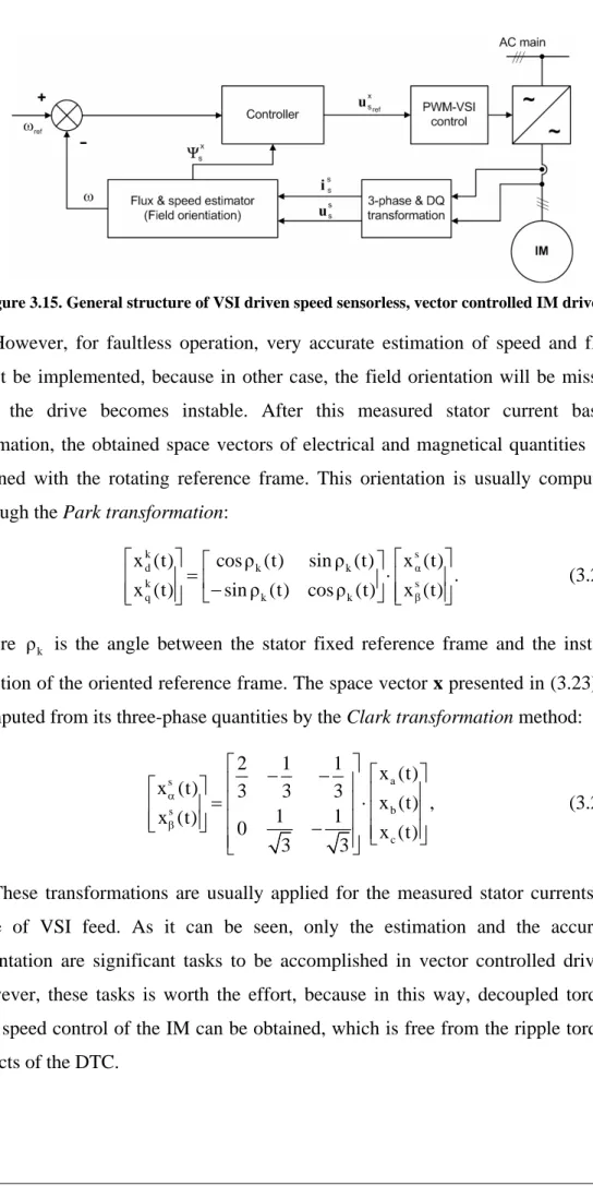
The transformation of the three phase quantities to a two-phase coordinate system and the field orientation is calculated through the Clark and Park transformations, whose details will be explained in the later sections.
2.6.
General dynamic properties of the model
The dynamical analysis of the motor model needs large spectrum of investigations which should cover another full paper in this topic. However, these investigations must be done before the true designing of the controller begins. For this reason, the full nonlinear analysis of the model has been completed in [38], but here only the main results and conclusions are mentioned.
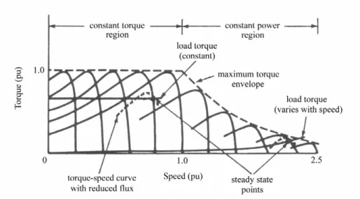
From equation (2.31), it is clear that the model is built up from first order subsystems. Thus, by considering each of these subsystems separately, the state variables tend to their equilibrium point without any overshoot and fluctuation, as well as their transition functions have purely exponential decrease. However, the inner cross effects caused by the multiplications between the state variables introduce high nonlinearities into the system, which cause oscillations in the dynamic behavior of the model. Moreover, the whole system dynamics can be separated into two operation interval: such as the startup and the steady state, in which the behavior of the model is different in terms of stability. During startup, the system shows instability till the electromagnetic torque
( )
Te has not reached a specific value called the pullout torque. This phenomenon exists, because a magnetic field has to be built up inside the motor to provide an adequate energy flow between the rotor and the stator subsystems. Thus, a high current impulse has to be provided to the motor, which quickly builds up the needed magnetic field and has enough energy to overcome the moment of inertia of the rotor. The difference in dynamic behavior of the two intervals can be seen in Figure 2.8 [18], where the interaction between the normalized T and e ω is plotted. It is clearly shown that during the direct startup, the function of torque / speed has large oscillations at first, which are dumped slowly till the system asymptotically reaches the equilibrium point(
)
nom nom, Te
ω as in the case of the steady state change. This plotted function also describes the step response of the transition function between the torque and speed.
It is another important fact that the relative degree between any inputs and any outputs of the system is not greater than 3. Based on this reason, the I/O
linearization of the model can be given easily in most of the cases, but for the load torque a very complicated virtual input and output functions have to be chosen for the linearization, which cause the accumulation of numerical error in practice. The effect of this property is analyzed in later sections. The zero dynamics of the system in contrast of the previous facts is stable for ω that makes possible to hold
load
T with the motor at 0 speed and control the full 4/4 operation range of the IM drive.
3.
Existing speed sensorless techniques
Today, several methods are known for the speed sensorless control of the induction drives, but each of these solutions has its own disadvantage beside its strong sides. In the past, there were arduous attempts to extract the speed or the position signal and to estimate the strength and the orientation of the flux field of an induction machine [18]. However, the first attempts have been restricted to techniques which are only valid in the steady state. These can be used in low-cost drive applications, not requiring high dynamic performance. But as the raging competition of the drive manufacturing companies has shaken this field up, a lot of new methods have been introduced which are applicable for high-performance applications in vector and direct torque controlled drives.
It is a common feature of the sensorless techniques that they depend on machine parameters, like the temperature of the motor, rotor resistance variations, frequency, etc. To compensate the parameter variations, various parameter adaptation schemes have been proposed in the literature. Unfortunately, conventional techniques are not suitable to achieve stable, very low speed operation in speed sensorless drives because the rotor speed directly based on the applied torque and the estimation of this fine balance is very problematic in this case, due to the parameter mismatch and noise. This task can only be solved by very difficult models that utilize various effects like the rotor slot harmonics, saliency, etc.[18]. This is the reason why beside the existing techniques there is a great search for new methods, like the controller whose implementation is the topic of this paper, which makes possible the control with a simple model that has smaller computational load than the recently used solutions in high performance drives. In the following parts, the most popular methods will be discussed briefly to have an outlook on the field of applied control of induction drives.
3.1.
Constant Volts per Hertz control
One way of dealing with the complex and nonlinear (NL) dynamics of the IM in adjustable speed drives is avoiding excitation at the eigenfrequency of the
frequency command as shown in Figure 3.1. The band limited stator frequency command signal then generates the stator voltage reference magnitude
ref s s
u while
its integral determines the phase angle
( )
ref ss .
u
Figure 3.1. Constant volt per hertz control
By examining the real voltage / rotor speed (given in frequency) characteristic of the motor presented in Figure 3.2, it can be clearly seen that during a large interval of the operation range, the relationship between ω and the applied voltage is linear in the case of constant load [20].
Figure 3.2. Voltage / frequency characteristic of the IM
It is also possible to effect the mmf. of the motor by changing the synchronous frequency of the voltage feed trough the PWM modulation of the inverter. Moreover, the T /e ω characteristics of the motor can be directly shifted along the frequency axis with the changing of the synchronous frequency, of course this is
only true theoretically, because the layout effects deform this relationship if the input frequency is too large or too low [5]. This is shown by Figure 3.3.
Figure 3.3. Torque / speed characteristics of the IM at different synchronous frequencies
The above mentioned properties can be derived mathematically as well. From (2.7), equation (3.1) is derived, by neglecting the resistive voltage drop s
s s
R i and, in view of band limited excitation, by assuming steady state operation with
s s dΨ / dt≈0. This yields s s s(t)= ωj s(t)⋅ s(t), u Ψ (3.1) or ref s s /ω =s const.
u (or v/f = const.) when the stator flux is maintained at its nominal value in the base speed range. Field weakening is obtained by maintaining
ref max
s
s =us =const.
u , while increasing the stator frequency beyond its nominal value. At very slow stator frequency, a preset minimum value of the stator voltage is programmed to account for the resistive voltage drop, which can be seen in Figures 3.1 and 3.2.
The signals ref s s u and
( )
ref s su are obtained to constitute the reference vector ref
s s
u of the stator voltage, which in turn controls a PWM modulator to generate the switching sequence of the inverter.
Since v/f drives operate purely as feed forward systems, the produced drive is absolutely robust, however, the mechanical speed ω differs from the reference
speed ωref when the machine is loaded. The difference is the slip frequency equal to the electrical frequency of the rotor currents. The maximum speed error is determined by the nominal slip, which is most commonly 3-5% for low power machines and less for high power. To compensate this, a load current dependent scheme can be employed to reduce the speed error [1].
If the system equations are derived in the stator fixed reference frame, letting
k 0 ω = . The result is s s s s s m s s r s r d (t) 1 L (t) (t) (t) , dt L = − − στ u Ψ Ψ Ψ (3.2) s s s s r m r r r r s s d (t) L (t) j (t) (t) (t). dt L στ ⋅ Ψ + Ψ = ω ⋅στΨ + Ψ (3.3)
From the (2.11) and (2.12) flux equations it can be clearly seen that
s s m s s s r s r L 1 (t) (t) (t) , L L = − σ i Ψ Ψ (3.4)
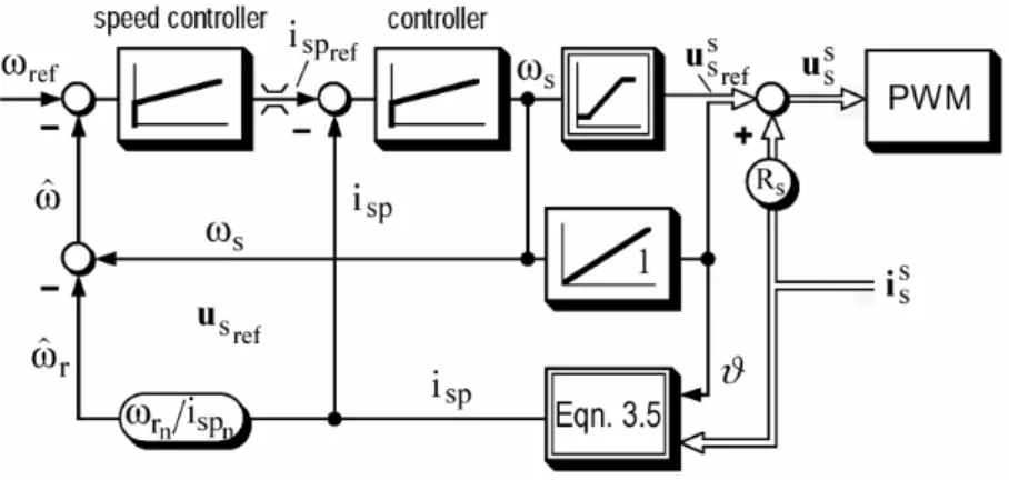
and the stator flux vector is directly generated by the integral of uss−Rs sis. The key quantity of this control concept is the active stator current i which is sp
ref ref ref s s s s s s sp s s s s s s (t)
i (t) (t) i (t) cos( ) i (t) sin( ), where ( (t)).
(t) α β
=u ⋅ i = α + α α = u
u (3.5)
It can be derived that i is proportional to the torque, thus if at the sp
nominal r
ω nominal slip the magnitude of the active iss is known, which is nominal sp
i then
the slip to be compensated can be estimated as:
nominal nominal r r sp sp (t) i (t). i ω ω ≈ ⋅ (3.6)
Based on this, the control structure demonstrated on Figure 3.4. provides favorable dynamic behavior by making the trajectory of the stator flux independent from of the stator current and the load.
Figure 3.4. v/f controller with slip compensation
Constant v/f control ensures robustness at expense of reduced dynamic performance which is adequate for applications like pump and fan drives. Their particular attraction is their extremely simple control structure which favors an implementation by a few highly integrated electronic components. These cost saving methods are specially important for applications at power below 5kW, but at high power, when the power components themselves dominate the cost, the implementation of more sophisticated control methods becomes available.
3.2.
Machine models
In practice, machine models are usually used to estimate the motor shaft speed to avoid the need of encoders or tacho generators and, in high performance drives with field oriented control, to identify the time varying angular position of the flux vector. In addition to this, the magnitude of the flux vector is estimated as well to ensure the effective operation of the drive.
Different machine models are employed for this purpose, and they are implemented in different manner to compute the unknowns depending on the problem at hand. Sometimes, by only the measured signals based solution of the differential equations of the model, with implemented real time numerical computation on a microprocessor, provides adequate performance, but in case of high expectations in optimality, these models are somehow enhanced by creating mathematical methods, called observers, which can improve the quality of the estimation of the desired values greatly. By applying these methods, the common
non speed sensorless control approaches become available to provide speed sensorless operation of the drive.
3.2.1. Direct reference models
Direct reference models are derived from the differential equations of the motor model either in stator fixed or field oriented representation. The accuracy of these models depends on the degree of coincidence which can be obtained between the model and the modeled system. Coincidence should prevail both in terms of structures and parameters. While existing analysis methods permit establishing of appropriate model structures in case of the IM, the parameters of such model are not always in good agreement with the corresponding machine data. Parameters may significantly change with temperature, or with the operating point of the machine. On the other hand, the sensitivity of a model to parameter mismatch may differ, depending on the respective parameter, and the particular variable estimated by the model, but it is always true that the slight computational load and easy structure of the reference machine models can guarantee only limited achievable performance.
Rotor models are derived from the relationship of the rotor winding either in stator (2.12) or in field coordinates (2.29). By example, in the stator fixed representation, the following equation gives possibility to compute the rotor flux:
s s s s r r r r r m s d (t) (t) j (t) (t) L (t). dt τ Ψ +Ψ = ω ⋅ τ Ψ + i (3.7)
If the previous differential equation is numerically solved, for example by the Euler method, then the desired value of Ψrs can be obtained to provide the rotor flux orientation by computing the angle of the rotor flux trough
s r s s s r r r s r s s r r 0, if (t) 0 (t) , if (t) 0 and (t) 0 (t) atan , (t) , if (t) 0 and (t) 0 α β α β α α β Ψ ≥ Ψ π Ψ < Ψ > ρ = + Ψ −π Ψ < Ψ < (3.8)
(
) (
2)
2s s s
s(t) = Ψrα(t) + Ψrα(t) .
Ψ (3.9)
Another important example is the stator approach, where from the (2.7) stator voltage equation (3.10) can be obtained.
(
)
t s s s s s s s 0 (t)=∫
u ( ) Rν − i ( ) dν ν Ψ (3.10)Equations (2.11) and (2.12) can be used to determine the rotor flux linkage vector Ψrs and the leakage vectorΨσs from which the penetrating field angle, and the magnitude of the flux linkage can be obtained:
(
)
(
)
t s r s s s r s s r s s s s s s m 0 m L L (t) ( ) R ( ) d L (t) (t) (t) . L L σ = ν − ν ν − σ = − ∫
u