DENSITY-BASED CLUSTERING OF HIGH-DIMENSIONAL DNA FINGERPRINTS FOR LIBRARY-DEPENDENT MICROBIAL
SOURCE TRACKING
A Thesis presented to
the Faculty of California Polytechnic State University, San Luis Obispo
In Partial Fulfillment
of the Requirements for the Degree Master of Science in Computer Science
by Eric Johnson December 2015
c 2015 Eric Johnson
COMMITTEE MEMBERSHIP
TITLE: Density-Based Clustering of
High-Dimensional DNA Fingerprints for Library-Dependent Microbial Source Tracking
AUTHOR: Eric Johnson
DATE SUBMITTED: December 2015
COMMITTEE CHAIR: Alexander Dekhtyar, Ph.D. Professor of Computer Science COMMITTEE MEMBER: Zoe Wood, Ph.D.
Professor of Computer Science COMMITTEE MEMBER: Christopher Kitts, Ph.D.
ABSTRACT
Density-Based Clustering of High-Dimensional DNA Fingerprints for Library-Dependent Microbial Source Tracking
Eric Johnson
As part of an ongoing multidisciplinary effort at California Polytechnic State Uni-versity, biologists and computer scientists have developed a new Library-dependent Microbial Source Tracking method for identifying the host animals causing fecal con-tamination in local water sources. The Cal Poly Library of Pyroprints (CPLOP) is a database which stores E. coli representations of fecal samples from known hosts acquired from a novel method developed by the biologists called Pyroprinting. The research group considers E. coli samples whose Pyroprints match above a certain threshold to be part of the same bacterial strain. If an environmental sample from an unknown host matches one of the strains in CPLOP, then it is likely that the host of the unknown sample is the same species as one of the hosts that the strain was previously found in. Clustering is a computer science technique for finding groups of related data (i.e. strains) in a data set. In this thesis, we evaluate the use of density-based clustering for identifying strains in CPLOP. Density-based clustering finds clusters of points which have a minimum number of other points within a given radius. We contribute a clustering algorithm based on the original DBSCAN algo-rithm which removes points from the search space after they have been seen once. We also present a new method for comparing pyroprints which is algebraically related to the current method.The method has mathematical properties which make it possible to use Pyroprints in a spatial index we designed especially for Pyroprints, which can be utilized by the DBSCAN algorithm to speed up clustering.
TABLE OF CONTENTS
Page
LIST OF TABLES . . . viii
LIST OF FIGURES . . . ix
CHAPTER 1 INTRODUCTION . . . 1
2 BACKGROUND . . . 7
2.1 Microbial Source Tracking (MST) . . . 7
2.1.1 Library-Dependent MST . . . 8
2.1.2 Representations . . . 10
2.2 Pyroprinting . . . 10
2.2.1 Pyrosequencing . . . 11
2.2.2 Gene Repetition and ITS regions . . . 12
2.2.3 Pyroprints . . . 14
2.2.4 Pearson Correlation . . . 15
2.2.5 Statistical Analysis and Strain Definition . . . 15
2.3 CPLOP: Cal Poly Library of Pyroprints . . . 17
2.4 Clustering . . . 19
2.4.1 OHClust!: Ontological Hierarchical Clustering . . . 19
2.4.2 DBSCAN: Density-Based Spatial Clustering of Applications with Noise . . . 20
2.5 Spatial Indexes . . . 22
2.5.1 Space Partitioning . . . 25
2.5.2 Bounding Volume Hierarchy . . . 27
2.5.3 Hybrid Spatial Index . . . 28
3 DESIGN . . . 29
3.1 Motivation And Goals . . . 29
3.2 Overview . . . 30
3.2.1 Speeding Up MST . . . 30
3.2.3 Scaling With a Growing Database . . . 31
3.3 Isolate Comparison . . . 33
3.3.1 Euclidean Distance of Pyroprint Z-Scores . . . 33
3.3.2 Considering Multiple DNA Regions . . . 36
3.4 Spatial Index . . . 37
3.4.1 Optimizations for use with DBSCAN . . . 38
3.4.2 Data Characteristics . . . 39
3.4.3 Construction . . . 40
3.4.4 Storage . . . 42
3.4.5 Algorithms . . . 44
3.5 Clustering . . . 47
3.5.1 Modified DSBCAN Algorithm . . . 49
4 IMPLEMENTATION . . . 54
4.1 Language and Libraries . . . 54
4.2 Overview . . . 55 4.3 Data Types . . . 56 4.4 Indexes . . . 58 4.5 DBSCAN . . . 60 4.6 Evaluation . . . 61 5 EVALUATION . . . 63 5.1 Evaluation Plan . . . 63 5.1.1 Performance Evaluation . . . 63 5.1.2 Strain Correctness . . . 64
5.1.3 Similarity to Current Method . . . 67
5.2 Isolate Sets . . . 69
5.3 Clustering Parameters . . . 70
5.3.1 DBSCAN . . . 70
5.3.2 Agglomerative Clustering and OHClust! . . . 71
5.4 Clusters Statistics . . . 71
5.5 Evaluation Results . . . 73
5.5.1 Performance Evaluation . . . 74
5.5.3 Similarity to Current Method . . . 79
6 CONCLUSION . . . 83
6.1 Future Work . . . 84
6.1.1 E. coli Strains . . . 84
6.1.2 Performance . . . 85
6.1.3 Additional Analysis Opportunities . . . 86
6.1.4 Correctness . . . 87
6.1.5 Applications . . . 88
LIST OF TABLES
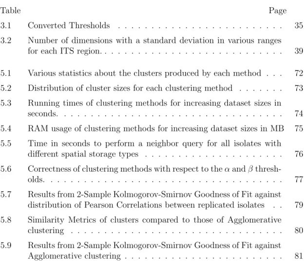
Table Page
3.1 Converted Thresholds . . . 35 3.2 Number of dimensions with a standard deviation in various ranges
for each ITS region. . . 39 5.1 Various statistics about the clusters produced by each method . . . 72 5.2 Distribution of cluster sizes for each clustering method . . . 73 5.3 Running times of clustering methods for increasing dataset sizes in
seconds. . . 74 5.4 RAM usage of clustering methods for increasing dataset sizes in MB 75 5.5 Time in seconds to perform a neighbor query for all isolates with
different spatial storage types . . . 76 5.6 Correctness of clustering methods with respect to theαandβ
thresh-olds. . . 77 5.7 Results from 2-Sample Kolmogorov-Smirnov Goodness of Fit against
distribution of Pearson Correlations between replicated isolates . . 79 5.8 Similarity Metrics of clusters compared to those of Agglomerative
clustering . . . 80 5.9 Results from 2-Sample Kolmogorov-Smirnov Goodness of Fit against
LIST OF FIGURES
Figure Page
2.1 A sample pyrogram, the result of pyrosequencing. . . 11
2.2 The rRNA operons in E. coli are present in seven copies, each of which has two Internal Transcribed Spacer (ITS) regions . . . 13
2.3 Beta distribution for pyroprints from the same isolate for ITS region 16-23 . . . 17
2.4 Example density-based cluster with MinPts=3 . . . 21
2.5 Pseudocode for the DBSCAN algorithm. . . 22
2.6 Pseudocode for the DBSCAN algorithm . . . 23
2.7 Binary Search Tree example . . . 24
2.8 Example KD-Tree . . . 26
2.9 Example R-Tree . . . 26
3.1 Pseudocode for the algorithm that constructs our spatial index. . . 45
3.2 Pseudocode for our range query algorithm . . . 46
3.3 Pseudocode for our range query algorithm . . . 47
3.4 Pseudocode for our range query algorithm . . . 47
3.5 Pseudocode for our modified DBSCAN algorithm . . . 52
3.6 Pseudocode for our modified DBSCAN algorithm . . . 53
4.1 SQL query for extracting isolates from CPLOP. . . 57
4.2 SQL query for finding the distribution of pairwise Pearson correla-tions from replicates in CPLOP. . . 62
5.1 The ontology definition used by OHClust! to generate clusters for the evaluation . . . 72
CHAPTER 1 INTRODUCTION
Clean sources of water are important for preventing the spread of diseases, and for maintaining the environment. One of the undesirable contaminants often found in bodies of water is feces[17]. The bacteria found along with fecal matter can make animals, including humans, sick. Environmental and Resource agencies are interested in finding the sources of fecal contamination. If the origin of contamination can be ascertained, then actions can be taken to remove or reduce the amount of fecal matter in the water.
The study of identifying and discriminating fecal bacteria in the environment is called Microbial Source Tracking (MST). MST techniques usually look for fecal indicator bacteria (FIB) in environmental samples[19]. These FIB are bacteria found in the digestive tracts of animals, called hosts, that sometimes leave the animals along with fecal matter. Investigators can look at the quantity of FIB in an environmental sample to estimate the amount of fecal contamination in the sampled environment[17]. Additionally, they can examine individual bacteria found in the sample and try to determine what host species they came from[17]. Generally, investigators are not interested in finding the exact individual host from which the bacterium came, but instead are satisfied with knowing the species of the host.
At the intersection of the fields of Computer Science and Biology lies a method of MST called library-dependent MST[19]. Library-dependent MST works off the assumption that there exist subgroups of an FIB species, called strains, which are only found in certain host species[17]. The method starts with the collection of a large number of bacteria samples from fecal matter from a known host species. Representations of these bacteria are stored in a database along with the information
about their provenance. Once the database is established, MST is performed by comparing environmental samples from unknown hosts to the samples stored in the database with the hope of finding a match. If matching bacteria are found, then researchers can look up the host species of the matching sample in the database and use that as evidence that the unknown sample came from the same host species.
Simply determining that two bacteria are of the same species is not necessarily enough to determine that two samples of FIB came from the same host species. In fact, a common FIB species used for MST,Escherichia coli (E. coli), is found in the guts and fecal matter of many host animals[17]. Instead, researchers must determine that the bacteria both came from the same subgroup of the species. The idea is that the more closely related two individuals are, the more recently they came from a common ancestor and thus the more likely they came from the same host species. Any meaningful subdivision of bacteria beyond species like this is called a strain. MST research groups formally define their notion of a strain by picking a metric of similarity and a threshold at which they are confident that bacteria are as closely related as their metric can determine; maximizing the probability that the bacteria came from a common ancestor and thus the same host.
Many methods can be used to measure the similarity between two bacteria cul-tures. The methods can be classified by whether they look at the phenotypes of the bacteria or the genotypes. Phenotypic comparison looks at appearance or behavior of the bacteria, for example their reaction to a certain chemical[17]. Genotypic compari-son on the other hand looks at the actual DNA of the bacteria. Comparing genotypes can be more expensive but is generally more discerning[19], as similar appearance or behavior can be produced by different sequences of DNA.
As part of an ongoing multidisciplinary effort at California Polytechnic State Uni-versity, biologists and computer scientists have developed a new library-dependent
MST method. The Cal Poly Library of Pyroprints (CPLOP) is a database developed by the computer scientists to support a novel, cost-effective genotype representa-tion method for bacteria comparison developed by the biologists called Pyroprinting. CPLOP uses E. coli as it’s FIB, storing representations acquired by running this Pyroprinting method on E. coli samples. To increase discrimination ability of the method, each E. coli sample’s DNA is pyroprinted in two separate locations. The research group considers E. coli samples which match in both locations with a sim-ilarity above a certain threshold to be part of the same strain. If that strain has only been seen in one host species then they have good evidence that environmental samples matching bacteria in that strain are also from the same host species.[20]
The number of samples stored in the database for library-dependent MST in-fluences the confidence in matches found with unknown samples. As the size of the database increases, so does the time to search for matches. In the case of the naive search method, an unknown sample must be compared to every sample in the database. At the time of this writing, MST in CPLOP[13] still relied on this method. If the notion of strains were to be stored in the database, then unknown samples could be compared to groups of bacteria in the database instead of every individual bacterium, speeding up the search. Storing strains in the database would also facili-tate other kinds of research. Longitudinal studies, such as that performed by Emily Neal[15], look at strains observed in an individual over time and look for changes or patterns. Transference studies, such as that performed by Josh Dillard[7], look at samples from different hosts for strains found in both hosts.
The desire for a method of identifying strains from the set of bacteria in the database is clear. Clustering is a computer science technique for finding groups of related data (i.e. strains) in a data set. There are different definitions of which data is part of the same group, or cluster. This is similar to the variation in definition of a strain in biology. Thus the choice of clustering method must match the biologist’s
idea of what constitutes a strain for their research.
In previous work for CPLOP, Aldrin Montana developed a method of clustering called OHClust![14]. OHClust! is based on agglomerative hierarchical clustering and utilizes information about the provenance of samples to allow efficient addition to the known clusters through incremental updates. Unfortunately, OHClust! cannot run on the CPLOP servers which have meager memory resources. In addition, in his evaluation of the clusters identified by OHClust!, Montana was unable to determine if the clusters matched the biologist’s notion of strains.[14]
The work presented in this thesis provides an alternate solution for identifying strains which hopes to address the limitations of OHClust!. It evaluates density-based clustering for the use in identifying E. coli strains from pyroprints. Density-based clustering, as defined by DBSCAN[9] finds clusters where points have a minimum number of other points within a given radius. The DBSCAN algorithm can find clusters like this very efficiently, especially if the points are stored in a spatial index.
The contributions of this thesis are the following:
• A modified DBSCAN algorithm: This is the first time density-based clus-ters have been tried with CPLOP. The original algorithm for finding density-based clusters was DBSCAN. Many researchers have provided modified versions of this algorithm suited for different purposes. This thesis modifies DBSCAN, allowing for the removal of points from the search space after they have been seen once. This modification results in a 2x speedup for our use case.
• A faster method for comparing pyroprints: Prior to this work, pyroprints in CPLOP were compared with Pearson Correlation. Pearson correlation ig-nores certain differences in the pyroprints which are due to inconsistencies in the physical pyroprinting process. This thesis presents a new method for com-paring pyroprints which is algebraically related to the old method, allowing
reuse of previous statistical analysis. In addition we precomputed some inter-mediate values which speeds up comparisons with both the old method and the new method. The new method was chosen such that it has mathematical properties which make it possible to treat the pyroprints as if they were points in multidimensional space.
• A spatial index that works with E. coli pyroprints: The DBSCAN al-gorithm can take advantage of storing data in a special way to increase the efficiency. If the points being clustered are points in space, then they can be stored based off their position in space. This is called a spatial index. Spatial in-dexes can be searched quickly for points near another point. This thesis presents a spatial index tailored for the needs of the data in CPLOP. It supports dense, high-dimensional data, by partitioning the search space with multidimensional planes as well as storing bounding volumes for groups of data. It also supports multiple regions for each data point with separate search radii.
• Better evaluation metrics of clusters for CPLOP: Finally, this thesis contributes an evaluation of the clusters generated by this work as well as those generated by OHClust!. This evaluation was more thorough than that provided in Montana’s Thesis, and is able to quantify how well the clusters match the Biologist’s notion of a strain. Unlike Montana’s evaluation, this evaluation goes beyond measuring the similarity of clusters to those produced by another clustering method.
The rest of this document is organized as follows. Chapter 2 provides detailed background information about both the biology and computer science sides of the problem context. Chapter 3 provides a detailed explanation of the design for the solution presented along with this thesis, as well as rational for design decisions. Chapter 4 provides relevant details about the solution implementation along with
the benefits or limitations of particular implementation choices. Chapter 5 outlines the evaluation performed on the solution followed by the results of the tests and analysis of those results. Finally, Chapter 6 concludes the paper and suggests areas of improvement as well as ideas for other related avenues of research.
CHAPTER 2 BACKGROUND
This chapter provides context for the work presented with this thesis. Faculty from the Biology department at California Polytechnic University (Cal Poly) in conjunc-tion with Computer Scientists from Cal Poly have developed a new method of mi-crobial source tracking. This method is library-dependent and utilizes a novel DNA fingerprinting technique, called pyroprinting, developed at Cal Poly. The Biology de-partment has a desire to identify bacterial strains in the library. The work presented in this thesis fulfils that desire using clustering and spatial indexes. It is an alternate solution to OHClust! created by Aldrin Montana[14].
2.1 Microbial Source Tracking (MST)
The pyroprinting technique was developed by Biologists at Cal Poly as a tool for microbial source tracking (MST)[5]. MST is the study of identifying and discriminat-ing bacteria in the environment. Usually, the bacteria in question are found in fecal matter contaminating environmental resources such as bodies of water. MST tech-niques usually look for fecal indicator bacteria (FIB) in environmental samples[19]. These FIB are bacterial species found in the digestive tracts of animals, called hosts, that sometimes leave the animals along with fecal matter. Investigators can look at the quantity of an FIB in an environmental sample to estimate the amount of fecal contamination in the sampled environment[17]. Additionally, they can examine indi-vidual bacteria found in the sample and try to determine what host species they came from[17]. Generally, investigators are not interested in finding the exact individual host from which the bacterium came from, but instead are satisfied with knowing the
species of the host. The waste from a single animal has a minimal impact on the cleanliness of a body of water, while the waste from a whole group can have a large impact.
2.1.1 Library-Dependent MST
The MST method developed by the Biologists at Cal Poly is classified as library-dependent. Library-dependent MST lies at the intersection of the fields of Computer Science and Biology. Library-dependent MST works off of the assumption that there exist subgroups of an FIB species which are only found in certain host species[17]. The method starts with the collection of a large number of bacterial samples from fecal matter of a known host species. Representations of these bacteria are stored in a database along with the information about the samples provenance. Once the database is established, MST is performed by comparing environmental samples from unknown hosts to the samples stored in the database with the hope of finding a match. If matching bacteria are found, then researchers can look up the host species of the matching sample in the database and use that as evidence that the unknown sample came from the same host species.
Library-dependent MST is typically organized as follows:
1. Collection: The first step is to collect microbial samples from fecal matter of known origin. When collected, the host species of the fecal matter is recorded. Additional information such as location where the fecal matter was found, and date of the collection can be recorded if desired for additional analysis oppor-tunities, but is not necessary for MST.
2. Isolation: A sample of fecal matter contains many individual bacteria. Library-dependent MST uses individual bacterial cultures, or isolates, taken from these samples. The process used by the biologists at Cal Poly to isolate E. coli
bacteria from the rest of the sample is described by Black et al.[5]. Multiple isolates can be taken from the same sample. The isolates can be cultured and frozen to replicate them for future experiments.
3. Digital Representation: After a single bacterium is isolated, researchers must then obtain a digital representation of the isolate. These representations are meant to be compared to each other in order to determine whether the isolates they match can be distinguished from each other. There are many different methods of obtaining these representations, and different types of represen-tations that can result. Some examples are discussed in Section 2.1.2. The pyroprinting technique developed at Cal Poly is one of these methods.
4. Addition to Library: Next, the DNA representation is added to the library along with metadata about the isolate it represents. The metadata includes the information recorded in step 1, especially the host species of the origin sample. Additionally, information about the isolate, and parameters for the representation can be stored for bookeeping purposes, and to ensure consistency. 5. Forensics: Once the library has grown sufficiently large (through multiple iterations of the previous steps), the system can then be used for MST. An en-vironmental sample is collected and processed according to steps 2-3 to produce an E. coli isolate from an unknown host. The resulting representation of this isolate is then compared against the representations of isolates in the library. If it matches any isolates in the library, then researchers look up the metadata of those isolates. It is up to the researches to come to a conclusion based on the amount and variety of host information from matching isolates about what host the environmental isolate likely came from.
2.1.2 Representations
Many methods can be used to measure the similarity between two bacteria. The methods can be classified by whether they look at the phenotypes of the bacteria or the genotypes. Comparing genotypes can be more expensive but is generally more discerning[19], as similar appearance or behavior can be produced by different sequences of DNA.
Phenotypic comparison looks at appearance/behavior of the bacteria. The idea is that bacteria from the same host species have adapted their behavior for survival in the particular environment encountered in the guts of the host species. Exam-ple representations that capture these traits include, results from biochemical tests, antibiotic resistance, and profiles of the proteins found on the outer membrane.[17]
Genotypic comparison on the other hand looks at the DNA sequence from the bacteria. The idea is that the more closely the DNA of two individuals are, the more recently they came from a common ancestor and thus the more likely they came from the same host species. A naive representation would simply be the full DNA sequence of the bacteria, however that would be expensive and impractical for both creation and comparison of the representations. Instead, researchers take shortcuts like measuring the size differences of DNA fragments related to a specific location (ribotyping), or by sequencing only a small part of the DNA which is highly variable[19].
2.2 Pyroprinting
Pyroprinting is a novel method of bacterial representation developed at Cal Poly by Michael W. Black, Jennifer VanderKelen, Anya Goodman, and Christopher L. Kitts[5]. They created the technique to address the problem they saw of researchers needing to choose between representations with good discrimination, and
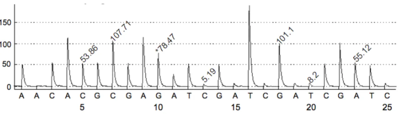
represen-Figure 2.1: A sample pyrogram, the result of pyrosequencing. Values represent the heights of peaks.
tations that were cheap/convenient to generate. Pyroprinting bridges the gap by providing both features. They are currently using pyroprints for MST with E. coli.
2.2.1 Pyrosequencing
Cal Poly’s pyroprinting method is based off of the DNA sequencing method called pyrosequencing. The method is popular because it is a cheap and efficient way to sequence short DNA fragments.
Pyrosequencing works on short sequences of DNA called regions. The region of DNA is determined by primers. A primer is a short fragment of DNA that binds to a specific complimentary DNA sequence, opening up the double helix. Two primers are needed, one to bind to the start of the region of interest and the other binding to the end. Once the primers are in place, DNA is copied from only that region. Pyrosequencing needs lots of copies of this region, so the region is repeatedly copied, or amplified, using the Polymerase Chain Reaction (PCR)[5].
Pyrosequencing is performed by a pyrosequencer machine which takes an amplified region of DNA and outputs a vector of data called a pyrogram as shown in Figure 2.1. This pyrogram can be used to reconstruct the sequence of nucleotides present in the sequenced region.
Pyrosequencing works by building a copy of the DNA strand and measuring the light given off by the resulting chemical reactions. Along with the DNA, the re-searchers provide a primer. The primer binds to a specific part of the DNA, and the DNA is copied sequentially starting from that location. The DNA is copied in stages called dispensations. One type of nucleotide is added per dispensation. Machines can usually run for around 100 dispensations. The machine records the amount of light emitted which is proportional to the number of nucleotides added to the copy during that dispensation. The resulting pyrogram is a graph of light emitted at each stage of the dispensation.
2.2.2 Gene Repetition and ITS regions
In order to be able to use pyrosequencing results to compare pyrograms between different isolates, the same region needs to be sequenced every time. This means the same primers need to be used every time. Primers are specific to specific DNA which means the sequenced region has to start with the same DNA sequence for every bacteria in the species. These regions exist in the DNA, and are called conserved regions. They are regions of DNA that are important genes which if mutated would result in the death of the cell, and thus those mutations would not be passed on to progeny. However, if only the conserved region is sequenced, all isolates would get the same representation. Ideally, the sequenced region would be highly variable, one which has little or no effect on the life of the bacteria. Regions between genes, or Internal Transcribed Spacers (ITS), as shown in Figure 2.2 fit this criteria. The way to get a representation from a region that is highly variable but is in the same place for different isolates is start pyrosequencing at the end of a conserved gene, then continue sequencing into the ITS region. The research group is interested in 2 ITS regions: ITS1 and ITS2. In the remainder of the thesis, each ITS region is referred to as the genes which surround it: ITS1 = 16-23 and ITS2 = 23-5.
Figure 2.2: The rRNA operons in E. coli are present in seven copies, each of which has two Internal Transcribed Spacer (ITS) regions. Thus PCR amplification of an ITS region will generate a population of mixed products to be pyrosequenced for generating a pyroprint. ITS1 and ITS2 are also referred to as the genes surrounding them: ITS1 = 16-23 and ITS2 = 23-5. Figure taken from [5].
E. coli, as well as many other bacteria, have multiple copies of certain genes located throughout their DNA for redundancy. Each copy is located at a specific location, called a locus (multiple loci). These replications mean that primers binding to these genes will actually bind to multiple different parts of the DNA. This means PCR will not replicate a single DNA region, but instead, in the case of E. coli, 7 different regions, as shown in Figure 2.2. While the conserved genes are identical in each of these loci, the ITS regions can differ between the loci. This means a single bacterial isolate can have different versions of the ITS mixed together when input to the pyrosequencer.
2.2.3 Pyroprints
Pyroprints are what the biologists at Cal Poly call the result of pyrosequencing a region of DNA with multiple loci. Because pyroprinting uses pryosequencing, the output of pyroprinting is a pyrogram. These pyrograms have different properties from pyrograms of true DNA sequences, and so are named pyroprints to differentiate the two. Specifically, pyroprints cannot be used to determine the DNA sequence of the region. This is because a pyroprint represents multiple variations (loci) of a given region. There is no way of knowing with this method whether all loci are the same, each is different, or something in between. Therefore, when examining a dispensation of a pyroprint, it is impossible to determine the distribution of added nucleotides among the loci. This property is why the biologists needed novel software and algorithms to perform MST with pyroprints.
In order to digitize a pyroprint, the biologists decided to take the maximum peak height from each dispensation. Other options were peak width and peak area. For-mally, the result is a vector ~pof length D
~
p= (p1, p2, . . . , pD−1, pD)
whereDis the number of dispensations of the pyroprint and eachpi is a positive real
number.
To increase discrimination ability of the method, each E. coli sample’s DNA is pyroprinted in two separate locations, 16S-23S and 23S-5S. In order to be considered indistinguishable, the representations of two isolates must match for both regions. Formally, an isolate’s representation is:
2.2.4 Pearson Correlation
Because pyroprints don’t translate to a specific DNA sequence, determining if a pair of pyroprints represents the same DNA is more difficult. Pyrograms have to be compared to pyrograms instead, and variations in hardware, PCR, and technician all result in different offsets and scales for each pyrogram. Comparisons require a metric that normalizes these variations. The metric used for comparing two pyroprints ~x and ~y is the Pearson Correllation ρ
ρ(~x, ~y) = 1 D D X i=1 (xi−µx)(yi−µy) σxσy
where D is the number of dispensation, and µx and σx are the mean and standard
deviation of the values of ~x at every dispensation respectively. µx = 1 D D X i=1 xi σx = v u u t 1 D D X i=1 (xi−µx)2
Pearson correlation returns a value between -1 and 1, where 1 is a perfect match, -1 is perfectly inverted and 0 means the pair is unrelated. For the purposes of MST, the research team is only interested in (non-inverted) matches. Because pyroprints are non-negative, Pearson correlations between them are always ≥0.
2.2.5 Statistical Analysis and Strain Definition
Due to noise in the pyrosequencing process, and by variations in the ratio of loci produced by PCR, two pyroprints will never match exactly. As such, the research team needed to determine a threshold of Pearson correlation above which 2 pyroprints are considered a match. Diana Shealy, a statistics student at Cal Poly, performed statistical analysis to determine thresholds for each ITS region[18].
In order to get a set of pyroprints which are supposed to match, the biologists made repetitive pyroprints of multiple isolates. They then took pairwise Pearson correlation values of pairs of pyroprints from the same isolate. This set of Pearson correlations was a sample of the distribution of Pearson correlations between pyroprints with the same DNA in the ITS regions.
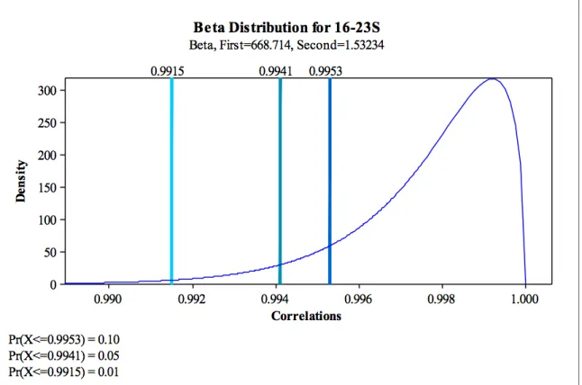
First, Shealy analyzed the effect of dispensation count on the Pearson correlation values. Pyrogram values get more noisy in later dispensations, because in the py-rosequencer machines, chemicals and proteins are not completely removed between each dispensation. So on one hand, using more dispensations decreased the Pearson value for isolates that are supposed to match. On the other hand, using less dispen-sations decreased the ability of Pearson correlation to capture differences between pyroprints from truly different sources. The research group decided to only use 95 and 93 dispensations of the pyrogram for the ITS regions 16-23 and 23-5 respectively. Shealy then fit a beta distribution to the sample distribution. Figure 2.3 shows the beta distribution fit to the pairwise Pearson correlations of pyroprints of the ITS region 16-23. From the beta distribution, Shealy calculated the percentages of false negatives at various Pearson correlation thresholds. Thresholds and false negatives for pyroprints of 16-23 are shown in Figure 2.3.
The choice of threshold affects the definition of a strain for the research group. The chance for false negatives (from higher thresholds) needed to be balanced with the chance for false positives (from lower thresholds). Shealy noted that:
“With pyroprints, we are more concerned with false positives, two pyro-prints that are said to be from the same E. coli strain when in fact they are not. We are less concerned with false negatives, or stating two pyro-prints are from different E. coli strains when they are actually from the same strain. The reason we are less concerned with false negatives is that hopefully any false negatives will be caught by a clustering algorithm and the false negative will then be appropriately classified.”[18]
Figure 2.3: Beta distribution for pyroprints from the same isolate for ITS region 16-23. Taken from [18].
Based on this analysis, the biologists chose two thresholds of for pyroprinting. Two isolates with a Pearson correlation above the α threshold 0.995 in both ITS regions are considered definitely similar. Two isolates with a Pearson correlation below theβ threshold 0.99 in either ITS region are considered definitely dissimilar. Isolates with a Pearson correlation between theα andβ thresholds may or may not be similar.[14]
2.3 CPLOP: Cal Poly Library of Pyroprints
The MST library created by the Computer Science and Biology departments at Cal Poly is called the Cal Poly Library of Pyroprints1 (CPLOP)[20]. CPLOP started as a prototype in a class at Cal Poly. After the class, Kevin Web, one of the students
from the class, completed CPLOP as his senior project. Later, Jan Soliman made extensive upgrades to CPLOP dubbed CPLOP 2.0[20].
CPLOP stores pyroprints and the provenance metadata associated with them in a relational database. The work of this thesis integrates with CPLOP. It takes its input from the pyroprint database, and stores its output there.
The primary use for CPLOP is microbial source tracking. MST is discussed in depth in Section 2.1. Other uses for CPLOP include facilitating longitudinal and transference studies. Longitudinal studies, such as that performed by Emily Neal[15], look at strains observed in an individual over time and look for changes or patterns. Transference studies, such as that performed by Josh Dillard[7], look at samples from different hosts for strains found in both hosts. Currently all use cases can and have been performed with the help of CPLOP. However, they are not convenient.
The first inconvenience is that MST tasks are slow. The forensics step of library-dependent MST (see step 5 in Section 2.1.1) requires finding all isolates with rep-resentations matching that of an isolate of unknown origin. The naive method of finding these matches compares the representation against every representation in the database. Pearson correlation is an expensive computation, especially with over 90 dimensions, and there are thousands of isolate representations in CPLOP. At the time of this writing, the latest MST algorithms used for CPLOP[13], still relied on this naive matching.
The inconvenience for longitudinal and transference studies is that strains are not integrated into CPLOP. Every time a researcher wants to look into a certain strain or a group of strains which are often seen together, the biologists must ask the computer scientists to run a clustering algorithm for them.
It is clear that storing strains in CPLOP would allow biologists to access them for longitudinal and transference studies without having to wait for computer scientists.
Additionally, storing the strains in a relational database (like CPLOP) would allow researchers to more easily view the isolates and metadata from strains with relational queries. Finally, storing strains in CPLOP would also enable faster MST forensics. Strains could have single representation[20] and unknown isolates would only need to be compared to each strain instead of each isolate, resulting in many fewer expensive Pearson correlation calculations.
2.4 Clustering
With the desire for storing strains of E. coli in CPLOP established, we now discuss methods for identifying them. Section 2.2.5 discusses the definition of a strain for pyroprinted E. coli arrived at through statistical analysis. Isolates whose represen-tations match above a certain threshold are considered members of the same strain. However, this threshold has false negatives, so strains must also include some isolates for which some pairwise comparisons are below the threshold.
Data clustering is the computer science task of grouping similar data together into clusters. It takes as input a set of data points, in this case pyroprints. The result of the task is a set of clusters and an N to 1 mapping from the input points to the resulting clusters. There are many different notions of a cluster and algorithms to create them.
2.4.1 OHClust!: Ontological Hierarchical Clustering
In previous work, Aldrin Montana created a clustering algorithm called OHClust! which addressed the need for strain identification[14]. OHClust! is based on agglom-erative hierarchical clustering. Agglomagglom-erative clustering starts with every point as its own cluster. Then at every step it combines the two closest clusters. This pro-cess ends when all clusters have been combined into a single cluster. The propro-cess
of combining clusters at each step produces a hierarchical view of the clusters. The hierarchy is cut at the desired level to determine the final clusters. This algorithm has O(N2) steps, and depending on the link type used to measure cluster distance, the overall algorithm can be O(N3). OHClust! uses average-link which uses the av-erage of all pairwise comparisons between two clusters as the distance between the clusters[14]. Average link agglomerative clustering is one of the like types that gives the overall algorithm a complexity of O(N3). OHClust! saw vast improvements in performance over standard average-link agglomerative clustering, but is still bounded atO(N3)[14].
The results and future work sections in Montana’s thesis talk about some of the limitations and issues of OHClust!. The big issue he mentions is a need for more testing and verification of his algorithm. Montana could not prove that the resulting clusters from OHClust! were similar to those of standard average-link agglomera-tive clustering, the algorithm previously used by the research team. Without an-other method of determine cluster validity, the correctness of OHClust! could not be determined[14].
Another limitation of Montana’s approach is the lack of integration with CPLOP. Currently, the biologists require assistance from the computer scientists to perform the clustering. This is because of performance problems with OHClust!. OHClust! needs more RAM than CPLOP’s servers can provide. Another limitation is that the runtime of OHClust! is very long. The work presented in this thesis tries to address these issues by focusing on performance.
2.4.2 DBSCAN: Density-Based Spatial Clustering of Applications with Noise
The work presented in this thesis uses a density-based notion of clusters and a modi-fied DBSCAN algorithm to identify strains. The notion of a cluster used by this work
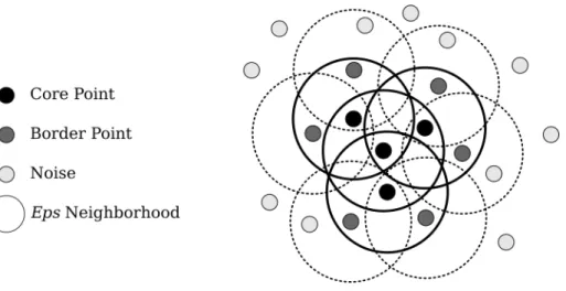
Figure 2.4: Example density-based cluster with MinPts=3
is defined by DBSCAN[9]. An example of a density-based cluster is shown in Figure 2.4. The DBSCAN definition of a cluster has two parameters, MinPts and Eps. It defines a neighbor of a point to be another point within a distance of Eps. Points are classified as either a core point, a border point, or noise. A core point is defined as a point with at least MinPts neighbors. A border point is defined as a point with less than MinPts neighbors but within Eps of a core point. All other points are defined as noise. A DBSCAN cluster is defined as a group of neighboring core points and the group of border points that neighbor that core.
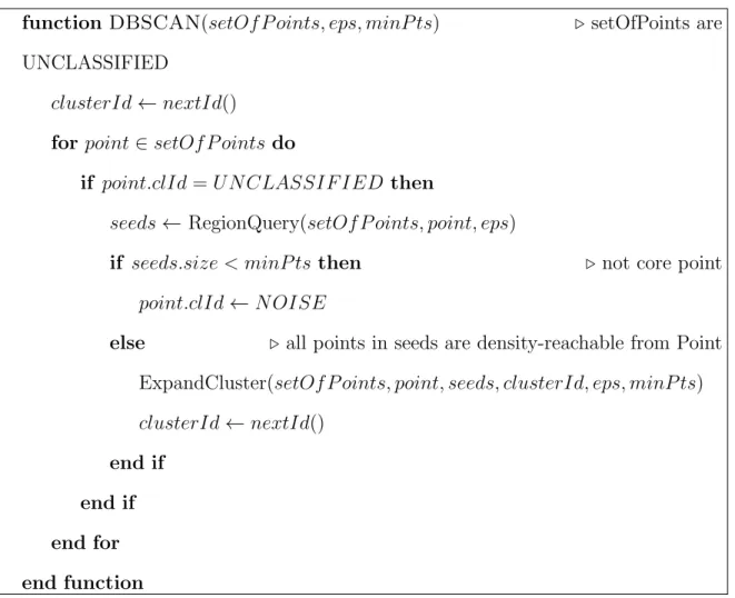
Pseudocode for the algorithm provided with the original DBSCAN paper is shown in Figures 2.5 and 2.6. The algorithm takes values forM inP tsandEps as input and uses that to classify every point into clusters. The algorithm runs in O(NlogN) given an O(logN) RegionQuery()[9].
Since the original paper came out, a few extensions of DBSCAN have been pub-lished. The OPTICS algorithm[1] provides a hierarchical clustering for density-based clusters. It generalizes away the Eps argument and only needs theM inP ts parame-ter. Another algorithm, IncrementalDBSCAN[8] significantly speeds up clustering if most of the points have previously been clustered.
function DBSCAN(setOf P oints, eps, minP ts) . setOfPoints are UNCLASSIFIED
clusterId←nextId()
for point∈setOf P oints do
if point.clId=U N CLASSIF IED then
seeds←RegionQuery(setOf P oints, point, eps)
if seeds.size < minP ts then . not core point point.clId←N OISE
else .all points in seeds are density-reachable from Point ExpandCluster(setOf P oints, point, seeds, clusterId, eps, minP ts) clusterId←nextId()
end if end if end for end function
Figure 2.5: Pseudocode for the DBSCAN algorithm.
2.5 Spatial Indexes
The clustering algorithm DBSCAN, described in Section 2.4.2, performs better with a O(logN) neighbor lookup. Such lookups require the points to be organized in an index optimized for the types of queries. In this case the queries are range-based which implies the use of a spatial index. Spatial indexes organize data to optimize for queries spatial in nature. An example of a query on a spatial index is finding all points within a geometric shape. If the shape is a sphere with radius Eps centered at one of the points, then the resulting points are all points within a distance Eps of the point at the center, ie. its neighbors.
function ExpandCluster(setOf P oints, point, seeds, clId, eps, minP ts) seeds.clId←clId
seeds.delete(point) while seeds6=∅do
currentP ←seeds.f irst()
result←RegionQuery(currentP, eps) if result.size≥minP ts then
for resultP ∈result do
if resultP.clId=U N CLASSIF IEDkN OISE then if resultP.clId=U N CLASSIF IED then
seeds.append(resultP) end if resultP.clID ←clId end if end for end if seeds.delete(currentP) end while end function
Figure 2.6: Pseudocode for the DBSCAN algorithm.
Spatial indexes are a special type of search tree. A search tree, as depicted in Figure 2.7 is composed of nodes. Most nodes have other nodes as children (inner nodes), but some nodes only contain data (leaf nodes). The nodes are arranged in a way such that when searching for certain data, only some children of each node need to be checked. In this case of the example search tree in Figure 2.7, the letter in a node comes alphabetically after all letters stored in the subtree as its left child, and
Figure 2.7: Binary Search Tree example. White nodes are inner nodes. Black nodes are leaf nodes.
alphabetically before all letters stored in the subtree as its right child.
A search is called a traversal and runs in O(logN) time. A traversal of the tree in Figure 2.7 searching for the letter P proceeds as follows. Traversals start at the root node of the tree, in this case M. At each step, the search letter is compared to the letter in the node. P is compared to M, and since P comes after M in the alphabet, the traversal moves to the node’s right child, V. Again, P is compared to V, and sinceP comes beforeV in the alphabet, the traversal moves to the node’s left child, R. Then, P is compared to R and sinceP comes before R in the alphabet, the traversal moves to the node’s left child,P. ThusP is found after only 3 comparisons, as opposed to 8 comparisons, one for each leaf node.
Most spatial indexes organize points by their location in a Euclidean space. This allows for efficient queries based on the Euclidean distance d(~x, ~y) between points.
d(~x, ~y) = v u u t D X i=1 (xi−yi)2
The math for Euclidean space scales to any positive number D dimensions.
points in Euclidean space. However Euclidean distances between these points would not be comparable to Pearson correlation. Section 3.3.1 explains how we can convert pyroprints into different ∼100 dimensional points where euclidean distances between these points are comparable to Pearson correlation of the original pyroprints. This allows us to store the points in normal spatial indexes in order to efficiently find points within a certain Pearson correlation threshold.
When choosing spatial indexes for such data, the curse of dimensionality comes in. Many spatial indexes degenerate into linear searches (searching every point) when the points have more than a few dimensions. The following sections describe some indexes designed specifically for high-dimensional data, while giving examples of some simpler ones.
2.5.1 Space Partitioning
The first class of spatial indexes is space partitioning. The general case is Binary Space Partitioning (BSP). BSP organizes data in a binary tree splitting the tree in half with plane (or hyperplane with more dimensions) each time. As implied by the name, each node of the tree ”partitions” the entire space.
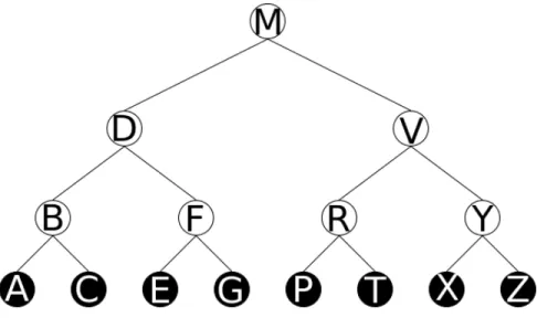
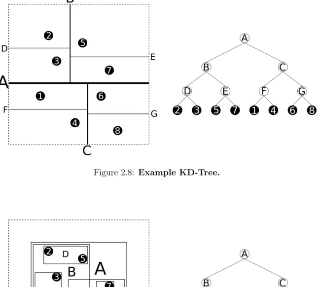
The KD-Tree, depicted in Figure 2.8, is a special case of BSP that partitions space with axis-perpendicular planes. At each node of the tree it partitions a single dimension. The dimension used for a node cycles as you move down the tree. KD-Trees are affected by the curse of dimensionality because partitioning each dimension x number of times requires a treex·Ddeep whereD is the number of dimensions [3]. The PK-Tree is based off the KD-Tree but addresses the issue with a large number of dimensions. It works like a KD-tree but with unnecessary nodes eliminated. Given some mild constraints on the data, the expected height of the tree can be bounded[21].
Figure 2.8: Example KD-Tree.
2.5.2 Bounding Volume Hierarchy
Another class of spatial indexes is a Bounding Volume Hierarchy (BVH). Instead of partitioning space, a BVH organizes data within bounding volumes. Each node in the tree is a volume that bounds all volumes and points in its sub tree. Depending on the shapes used, sibling nodes can have overlapping volumes even if the points they contain are disjoint.
The R-Tree, depicted in Figure 2.9, is a popular BVH that uses only rectangular volumes. The construction of an R-Tree allows for lots of overlap. R-Trees are subject to the curse of dimensionality because overlapping nodes becomes a bigger and bigger problem with more and more dimensions[10].
The R*-Tree is based on the R-Tree which addresses the issue of overlap. The construction of an R*-Tree tries to minimize overlap by reinserting points when a node gets too full[2]. The X-Tree is based on the R*-Tree, and addresses the issue of overlap a step further. X-Trees use supernodes which allow problematic points to be stored in internal nodes instead forcing them into a leaf node which would cause overlap.[4]
An alternative to the R-Tree family is the SR-Tree which uses the intersection of spheres and rectangles for the volumes of its nodes. This is based off the idea that volumes that better fit the points they contain are less likely to overlap with each other[11]. Another alternative is the TV-Tree. TV-Trees address the dimensionality issue by using only a few of the dimensions. They use the additional dimensions only when absolutely needed[12].
2.5.3 Hybrid Spatial Index
Another class of spatial index combines space partitioning and bounding volume hierarchy. An example of this is the Hybrid-Tree. It is based on the KD-Tree but the partitions can overlap requiring the subspaces to be treated as bounding volumes for searching[6].
CHAPTER 3 DESIGN
This chapter describes the algorithms contributed along with this thesis. The al-gorithms are the primary contribution of this thesis. The first section outlines the goals for the solution. Next is an overview of the solution design. Following that is a detailed look at each part of the solution.
3.1 Motivation And Goals
Chapter 2 describes the origin of the Cal Poly Library of Pyroprints (CPLOP), a tool for a new method of Microbial Source Tracking (MST) developed by the biology department at Cal Poly. Section 2.3 explains the benefits of identifying strains of E. coli among the isolates stored in CPLOP.
The algorithms we contributed identify and analyze strains from the pyroprints stored in the CPLOP. The goals for the solution were (1) to allow for faster MST, (2) to allow strain analysis in an easy to understand form, and (3) to scale with the database as it is incrementally updated with new pyroprints.
The ultimate purpose of this thesis is to provide an alternative solution to that provided by Aldrin Montana in his thesis[14]. His solution, OHClust!, described in Section 2.4.1, was motivated by the same original need, and had similar goals. Unfortunately, the meager computational resources allocated to the CPLOP server could not run OHClust!. As such, a secondary goal for the design of this thesis was to have light resource requirements.
3.2 Overview
We started our design with the desire to try density-based clustering for strain iden-tification to see how it compares to an agglomerative approach like OHClust! when applied to the data collected by the biologists at Cal Poly stored in Cal Poly Library Of Pyroprints. Many of the design decisions revolve around ensuring that we can leverage the performance benefits of density-based clustering.
3.2.1 Speeding Up MST
The first goal for our solution was to allow for faster MST. This is very useful, because the naive method of matching isolates for MST, comparing an unknown isolate to every isolate in the database, scales poorly with the growing library of isolates.
As described in Section 4.8 of Jan Soliman’s thesis[20], it is possible to use iden-tified strains to speed up the MST process. By using a representative isolate for each strain, matching an unknown isolate only requires looking at each strain representa-tive instead of every isolate.
This thesis contributes to this speed up by identifying strains and storing them in CPLOP. Section 4.7.2 of Soliman’s thesis[20] describes the relational data model for storing strains in CPLOP.
3.2.2 Allowing Strain Analysis
The second goal for our solution was to provide analysis of strains in an easy to understand form. The purpose of analyzing bacterial strains in the library is to find similarities between bacterial representations. These similarities signify pairs of isolates that have some identical sequences of DNA and likely share a recent common ancestor. This allows the biologists to look for patterns in the metadata of related
isolates. With metadata such as time and location of the samples, the biologists can then ask questions like ”where has this strain of bacteria been seen?” and ”how has that changed over time?”
OHClust! coupled the identification of strains with their analysis. As such, when Montana was unable to verify the validity of the identified strains, the analysis could not be used either. Hoping to avoid a similar fate, and for the sake of simplicity, we decided to decouple strain identification and analysis in our solution. We designed a tool that could be used to analyze strains found by any clustering method. Our solution is to store identified strains in CPLOP, allowing researchers to use SQL queries on CPLOP to analyze those strains.
3.2.3 Scaling With a Growing Database
The third goal for our solution is to grow with the database. The biologists are continually gathering new samples and sequencing them into pyroprints which are added to the database. Montana’s solution for this goal was to make OHClust! incremental. The time to cluster a few new pyroprints in OHClust! is much faster than clustering everything from scratch. For our solution however, we decided not to use an incremental algorithm. This is a simpler solution that we thought would still scale with the database due to the efficiency of the clustering algorithm we chose, DBSCAN.
DBSCAN has a runtime complexity of O(NlogN) compared to agglomerative clustering which has complexity of up toO(N3) (as in the case of OHClust!) depend-ing on the intercluster distance metric used. The O(NlogN) complexity of density-based clustering algorithms depends on the use of spatial indexes withO(logN) range queries.
a spatial index to store our data, we had to find the relationship between Pearson correlation and Euclidean distance. In Section 3.3.1 we derive the following relation-ship:
ρ(~x, ~y) = 1−d(z~x, ~zy) 2
2D
where ~x and ~y are pyroprints, ρ is the Pearson correlation, d is Euclidean distance, ~
zx and z~y are the z-scores of~xand ~y, and D is the number of dimensions.
Using this formula, we converted our α and β thresholds, described in Section 2.2.5, from Pearson correlation to Euclidean distance of Z-scores. Our solution pre-computes the z-scores for each pyroprint. Then during clustering, it calculates the Euclidean distance between pairs of pyroprints and compares the value to the con-verted thresholds.
The next step was to decide on the spatial index to use for our clustering. Spatial indexes are notoriously bad at scaling to high-dimensional spaces. Unfortunately, the 93-95 dispensations of our pyroprints is well within the classification of dimensional. Common aspects of spatial indexes that we needed to avoid for high-dimensional data were having overlaping nodes, and splitting dimensions indepen-dently.
The best spatial indexes designed for high-dimensional data we could find are described in Section 2.5. They were all designed to store that data persistently on disk. Because all of our data should fit in RAM for the foreseeable future, we decided not to persist our index. As such, we did not use the previous solutions and instead designed our own. The index we designed was tailored for our data and the query pattern of the DBSCAN algorithm. It is described in Section 3.4
3.3 Isolate Comparison
There are two components to comparing isolates. First is the comparison of pyroprints from the same DNA region. Second is the way comparisons from all DNA regions are used to come to a decision on similarity.
3.3.1 Euclidean Distance of Pyroprint Z-Scores
Spatial indexes generally operate on data existing in Euclidean space. The pyroprints could be thought of as points in an D-dimensional space where D is the number of dispensations. The distance between two points in Euclidean space can’t be converted to the Pearson correlation between two points which was previously used by those working with CPLOP. The calculation of the Pearson correlation uses the average and standard deviation of the dimensions in a point, but Euclidean distance discards the information needed to find the average and standard deviation. There is a type of spatial indexes called a m-tree which can operate on arbitrary metrics[16]. Unfor-tunately, the Pearson correlation does not fit the criteria of a proper metric which is required by m-trees. Specifically, Pearson correlation violates the triangle inequality property.
The reason the biologists use Pearson correlation, as described in Section 2.2.4, is because it statistically normalizes the data. We needed Euclidean distance for use in a spatial index, and we needed to use statistical normalization for comparison validity. Since the biologists had already determined meaningful thresholds for Pearson corre-lation, we hoped to be able to leverage that by finding a relationship between Pearson correlation and Euclidean distance with statistical normalization. The following is a derivation of that relationship.
We start with the equations for Pearson correlation ρ and Euclidean distance d: ρ(~x, ~y) = 1 D D X i=1 (xi−µx)(yi−µy) σxσy d(~x, ~y) = v u u t D X i=1 (xi−yi)2
where D is the number of dimensions, and µx and σx are the mean and standard
deviation respectively. µx = 1 D D X i=1 xi σx = v u u t 1 D D X i=1 (xi−µx)2
We notice that the inner terms of Pearson correlation are z-score normalizations, z(xi) =
xi−µx
σx
and plug in z(xi) into the distance equation for x and y and simplify.
d(z~x, ~zy) = v u u t D X i=1 xi−µx σx − yi−µy σy 2 = v u u t D X i=1 xi−µx σx 2 −2 xi−µx σx yi−µy σy + yi−µy σy 2 = v u u t D X i=1 xi−µx σx 2! + D X i=1 yi−µy σy 2! −2 D X i=1 xi−µx σx yi−µy σy = v u u t P (xi−µx)2 σx2 + P (yi−µy)2 σy2 −2 D X i=1 (xi−µx)(yi−µy) σxσy
We notice the the sums look like parts of the equations for σ and ρ. Solving the equations for the sums gives us:
D X i=1 (xi−µx)2 =D·σx2 D X i=1 (xi−µx)(yi−µy) σxσy =D·ρ(~x, ~y)
ITS region 23-5 16-23
α β α β
ρ(~x, ~y) 0.995 0.99 0.995 0.99
D 93 95
d(z~x, ~zy) 0.9644 1.3682 0.9747 1.3784
Table 3.1: Converted Thresholds.
and we substitute those back into our d(z~x, ~zy) equation and simplify.
d(z~x, ~zy) = s D·σx2 σx2 + D·σy 2 σy2 −2D·ρ(~x, ~y) =p2D−2D·ρ(~x, ~y) =p2D(1−ρ(~x, ~y)) Thus the relationship between ρ and d is:
d(z~x, ~zy) = p 2D(1−ρ(~x, ~y)) or ρ(~x, ~y) = 1− d(z~x, ~zy) 2 2D
Using this formula, we converted ourα andβ thresholds from Pearson correlation to Euclidean distance of Z-scores, shown in Table 3.1. Because the conversion depends on number of dimensions D, the threshold for distance is different for each region despite being the same for Pearson correlation.
Our solution precomputes the z-scores for each pyroprint. Then during clustering, it calculates the Euclidean distance between pairs of pyroprints and compares the value to the converted thresholds.
3.3.2 Considering Multiple DNA Regions
The biologists realized that pyroprints from a single region of DNA was not enough to be able to determine if two isolates are are the same or not. So for each isolate there are actually two pyroprints, one from each of two different regions. Isolates are considered equal only if the pyroprints from both regions match under the threshold. Because the two regions have different thresholds, the distances can’t be combined into one distance, to be compared against a single threshold. Instead, decisions on similarity need to take into account the distances between every region.
The first idea we considered was to cluster isolates twice, once for each region, then to take intersections of the cross product of both sets of clusters. Isolates that were in the same cluster for each region are in the same cluster of the combined regions. This design would have a couple benefits. First, it would be simple to implement because the comparison for two pyroprints is just distance. Second it could provide additional analysis opportunities for the biologists, who could look for patterns within a single region, or find relationships between strains based on which other strains share one of the region clusters. The primary drawback of this design is additional computation. At first glance, clustering twice would be twice as much work. But on top of that the clustering itself becomes more expensive because the range queries on a single region return a significant portion of our data which results in worst case performance complexity O(N) from the spatial index, making the full algorithm O(N2) instead of O(N logN).
The second idea we considered was to combine the regions and do a single cluster-ing of both regions at the same time. The benefits and drawbacks of this approach are the inverse of those of the first approach. Performance is better because the spatial index has more information on which to trim branches of the tree. Design complexity is higher because calculations and decisions during the query need to take into
ac-count two independent regions. This also means that the query algorithm takes two radii as input, one for each region, instead of the normal one radius.
We decided to use the second approach for this work. While the opportunity for extra analysis would be nice, it wasn’t specifically asked for, while good performance was. Additionally, the analysis would likely be performed infrequently, and thus the extra computation would be wasted most of the time. Perhaps in the future the ability to make such analyses could be added separately from the basic strain identification.
3.4 Spatial Index
All of the design for strain identification revolved around the spatial index. The data was transformed into z-scores and the thresholds converted for Euclidean distance so that a spatial index could be used. Density-based clustering gets its performance from leveraging a spatial index.
Our primary concern with choosing a spatial index is the fact that our data is high-dimensional. Most spatial indexes scale poorly with dimensions. Common aspects of spatial indexes that we needed to avoid for high-dimensional data were having overlapping nodes, and splitting dimensions independently.
The best spatial indexes designed for high-dimensional data we could find are described in Section 2.5. They were all designed to store that data persistently on disk. Because all of our data should fit in RAM for the foreseeable future, we decided not to persist our index. As such, we did not use the previous solutions and instead designed our own.
Because we decided not to have a persistent index, it must be built from scratch whenever we want to cluster the data. Therefore, we must choose a spatial index which can be built quickly. Specifically, the complexity should not be worse than the
complexity of the clustering,O(NlogN), otherwise building the tree would dominate the total runtime as the dataset scales.
Designing our own spatial index allows us to make some optimizations for its use in DBSCAN as well as for the specific characteristics of our data.
3.4.1 Optimizations for use with DBSCAN
In order to be used by DBSCAN, the spatial index needed to provide a range query. A range query takes a query point, and a range as input and returns all data points within range of the query point. The query can be thought of as a hypersphere with it’s center at the query point with a radius of the query range. All points that lie inside that hypersphere are returned.
The DBSCAN algorithm queries the spatial index in a unique pattern. First, all queries are centered at a point in the database, as opposed to an arbitrary point with all queries having the same range. Second, each point is only queried once, and nearby points are processed soon after each other.
Our spatial index query takes some shortcuts by realizing that once a point and all of its neighbors have been processed, DBSCAN will never make another query that would return that point. In addition, we modified the DBSCAN algorithm to keep track of the neighbors seen for each unprocessed point. This means that it will never need to see any points more than once. These modifications are described in Section 3.5.1.
By only committing to returning points that have not been previously returned we can get away with only searching points that haven’t been returned yet. By removing points from the spatial index after they are returned, future queries will have fewer points to search through.
[0.0,0.25) [0.25,0.5) [0.5,0.75) [0.75,1.0) [1.0,1.25) [1.25,∞)
23-5 37 45 7 0 3 1
16-23 46 39 6 1 0 2
Table 3.2: Number of dimensions with a standard deviation in various ranges for each ITS region. The deviations are calculated between z-scores, not the original pyroprints.
3.4.2 Data Characteristics
Our data has some characteristics that make it difficult to use in a spatial index. The points have very little spread in most dimensions. As shown in Table 3.2, standard deviations between points in a single dimension are less than 0.5 for most dimensions. Compared to the range of the query of 0.96 or 0.97 for the α thresholds of 23-5 and 16-23 respectively, the difference between points in a single dimension usually won’t be enough to exclude a point from the query results. Unfortunately, we can’t ignore any single dimension because those small differences add up over ∼100 dimensions. Unfortunately, this means that when traversing the tree, the algorithm will branch to multiple children to a greater depth, until many dimensions have been looked at.
In order to keep the tree depth low, our design splits points based on multiple dimensions per level. This is common in spatial indexes such as the popular quadtree and octree, however, that approach increases the number of children of each node exponentially (2D) where Dis the number of dimensions split at that level. Splitting all ∼100 dimensions in one node would be impractical with 290 children. We could instead split only a few different dimensions at each level of the tree, but the tree would still have the same number of leaves after splitting each dimension once. Since 290 leaves is more than the number of data points we could ever possible hope to add to the database, the majority of those leaves would be wasted. In addition, the range
query would intersect many of these children, causing the algorithm to traverse down exponentially many paths. This is somewhat offset by the reduced depth of the tree, but it is not ideal. TheO(logN) performance of spatial data queries assumes that at the majority of nodes, only one child is further traversed.
What we decided to do instead was split multiple dimensions dependently. That is to split once but have that one split cover multiple dimensions. This means that the split plane won’t be axis aligned. The idea is that by changing the angle of the split plane the average distance from points on either side to the split plane will increase. This increase depends on a correlation between dimensions i.e. points with low values (relative to other points) in one dimension, also tend to have low values (relative to other points) in another dimension. Inverse correlations work too, as long as most points with low values in one dimension have high values in another. Fortunately, the data in our library does exhibit correlations between some dimensions.
3.4.3 Construction
This section describes the remaining details of the design of the spatial index. Since the tree is not persistent, we can construct the tree with knowledge of all the points. Instead of constructing the tree by adding one point at a time and splitting nodes when they get too big (like many bounding volume hierarchy indexes) or picking arbitrary split criteria ahead of time (like many spatial partitioning indexes), our design looks at all points in a (sub)tree then partitions them.
As discussed in Section 3.4.2, our spatial index partitions points by finding a plane that splits the data in multiple correlated dimensions. The dimensions are chosen by picking the single dimension in which the points are most spread apart, as determined by standard deviation, and then choosing a number of other dimensions based on a combination of how correlated they are to the first dimension and how spread those
dimensions are. Specifically it chooses the N dimensions with the highest values for |ρ|·σ, whereρis the Pearson correlation of data values for a dimension with the values for the dimension with the most spread, σ is the standard deviation for a dimension, and N is a parameter to the construction algorithm.
Each dimension is only split once per path down the tree. The true distance to a node is not simply the distance to the split plane of that node, but actually the distance to the intersection of the planes of all the ancestors of the node. Instead of finding those intersections and calculating the distance to the complex shape that results, we can combine the distances to individual planes using Euclidean distance dcombined =
p
d12+d22. In order to combine distances from multiple split planes during queries (the split planes from a node and all of its ancestors), each of those planes must be perpendicular to all of the others. The simplest way to guarantee this is to enforce that no plane shares any dimension with another. Dimensions will be reused in the planes of nodes that aren’t direct ancestors or descendants as distances to those planes will not be combined during queries.
After picking the dimensions, our construction algorithm chooses a hyper-plane using linear regression between each dimension and the dimension with the most spread. The formula determines the slope b =ρ· σx
σy and intercept i = sx−b·sy of the regression linea·x+b·y+i= 0 wherexis the value of a point in the dimension with greatest spread,yis the value of the point in the other correlated dimension, and a:= 1. The interceptidetermines the position of the split plane, and is calculated for a points on the plane. We tried two options fors, the mean of each dimension, and the median point in relation to the split plane. The mean is less work to calculate, thus results in faster construction. The median point results in a balanced tree, thus faster queries. Since the performance of our spatial index is dominated by the queries and not the construction, we chose to use the median point.
The algorithm finds an equation of a hyper-plane by combining these linear re-gression equations into a forma·x+b·y+. . .+c·z+i= 0 wherexis the dimension with the most spread (again with a := 1) and each subsequent term is a correlated dimension multiplied by the slope (b·y) of the linear regression with the first dimen-sion. The intercept i is simply the sum of the intercepts from the linear regression for each correlated dimension.
In order to partition the points based on the hyper-plane, we needed a function that, given a point < x0, y0,· · · , z0 > and the equation for the plane (a·x+b·y+ . . .+c·z +i = 0), would return which side of the plane it was on. We used the equation for signed distance from a plane for this purpose as well as for the spatial query algorithm. The formula for the distance is
d= a·x0√+b·y0+. . .+c·z0+i a2+b2+. . .+c2
The result of this equation is signed, and that sign determines which side of the plane a point is on. For the purpose of partitioning, only the sign matters, so we can ignore the denominator. Since the plane is only in a subset of the dimensions, the ”point” we input to the function is made up of only those dimensions from the real data point, in the same order as they are used in the plane equation.
3.4.4 Storage
After deciding which points go in which child of a tree node, the algorithm has to encode spatial information about those children for the query to use. The two most common methods of doing this are (1) storing the plane used to split the data i.e. spatial partitioning, and (2) storing a bounding volume for each child fit to the data points withini.e. bounding volume hierarchies. The benefits of storing the split plane are that it generally takes less storage space, and it guarantees no overlap between children which can be a problem with bounding volumes. Bounding volumes come