E¢ cient parallelisation of Metropolis-Hastings
algorithms using a prefetching approach
Ingvar Strid
Dept. of Economic Statistics and Decision Support,
Stockholm School of Economics
SSE/EFI Working Paper Series in Economics and Finance No. 706
2009-12-02 (revised version)
Abstract
Prefetching is a simple and general method for single-chain parallelisation of the Metropolis-Hastings algorithm based on the idea of evaluating the posterior in par-allel and ahead of time. Improved Metropolis-Hastings prefetching algorithms are presented and evaluated. It is shown how to use available information to make better predictions of the future states of the chain and increase the e¢ ciency of prefetching considerably. The optimal acceptance rate for the prefetching random walk Metropolis-Hastings algorithm is obtained for a special case and it is shown to decrease in the number of processors employed. The performance of the algo-rithms is illustrated using a well-known macroeconomic model. Bayesian estimation of DSGE models, linearly or nonlinearly approximated, is identi…ed as a potential area of application for prefetching methods. The generality of the proposed method, however, suggests that it could be applied in other contexts as well.
Keywords: Prefetching, Metropolis-Hastings, Parallel Computing, DSGE model, Optimal acceptance rate, Markov Chain Monte Carlo (MCMC)
Email adress: [email protected]. Tel: +4687369232. Fax: +468348161. Permanent adress: Stock-holm School of Economics, P.O. Box 6501, SE-113 83 StockStock-holm, Sweden. I thank Sune Karlsson, John Geweke, Ingelin Steinsland, Karl Walentin, Darren Wilkinson and Mattias Villani for comments and dis-cussions that helped improve this paper. I also thank seminar participants at Sveriges Riksbank, Örebro University and the14thInternational Conference on Computing in Economics and Finance in Paris. The
Center for Parallel Computers at the Royal Instititute of Technology in Stockholm provided computing time for experiments conducted in the paper.
1
Introduction
E¢ cient single-chain parallelisation of Markov Chain Monte Carlo (MCMC) algorithms is di¢ cult due to the inherently sequential nature of these methods. Exploitation of the conditional independence structure of the underlying model in constructing the paral-lel algorithm and paralparal-lelisation of a computationally demanding likelihood evaluation are examples of problem-speci…c parallel MCMC approaches (Wilkinson (2006); Strid (2007b)). The prefetching approach and ‘automatic’parallelisation using parallel matrix routines are more general approaches (Brockwell (2006); Yan et al. (2007)).
In this paper we propose simple improvements to the prefetching Metropolis-Hastings algorithm suggested by Brockwell (2006), which is a parallel processing version of the method originally proposed by Metropolis et al. (1953) and later generalised by Hastings (1970). As the name suggests the idea of prefetching is to obtain several draws from the posterior distribution in parallel via multiple evaluations of the posterior ahead of time. It is assumed that the proposal density depends on the current state of the chain, such that the future states must be predicted. We show how the random walk Metropolis-Hastings (RWMH) prefetching algorithm can be improved by utilising information on the acceptance rate, the posterior and the sequence of realised uniform random numbers in making these predictions. It is also explained how the optimal acceptance rate of the RWMH algorithm depends on the number of processors in a parallel computing setting.
When the proposal density does not depend on the current state the prediction problem vanishes. Parallelisation of the Metropolis-Hastings algorithm is simpli…ed considerably and reminiscent of parallelisation by running multiple chains. The attractiveness of the independence chain Metropolis-Hastings (ICMH) algorithm is therefore obvious from a parallel computing perspective.
The main focus here is on developing e¢ cient prefetching versions of the one-block RWMH algorithm. The one-block case is the most attractive setting from a pure parallel e¢ ciency perspective. Further it allows for a simple exposition of concepts and algorithms. The prefetching method generalises to the multiple blocks case, as we describe brie‡y. In general, however, we expect it to be less e¤ective in that context, at least in situations where some of the full conditional posteriors can be sampled directly using Gibbs updates. Prefetching has obvious limitations in terms of parallel e¢ ciency but there are at least three reasons why the approach is still interesting. First is the generality of the one-block prefetching method; it is largely problem independent. Second, prefetching is easy to combine with other parallel approaches and can therefore be used to multiply the e¤ect of a competing parallel algorithm, via construction of a two-layer parallel algorithm. As a result, even if prefetching, by itself, is reasonably e¢ cient only for a small number of processors its contribution to overall performance is potentially large. Finally, the method is easy to implement and provides a cheap way of speeding up already existing serial programs.
tion of Dynamic Stochastic General Equilibrium (DSGE) models. Estimation of large-scale linearised DSGE models or nonlinearly approximated DSGE models of any size are computationally demanding exercises. This class of models is also chosen because the one-block RWMH algorithm has been the predominant choice of sampling method, for reasons explained below.
Despite the focus on macroeconomic models the generality of the prefetching approach suggests that the methods should be useful in other contexts. Estimation of long mem-ory time series models and -stable distributions using the RWMH algorithm are direct examples (Brockwell (2006); Lombardi (2007)). For latent variable models we argue that prefetching is suitable in conjunction with marginalisation techniques whereas other paral-lel approaches are required with sampling schemes based on data augmentation and Gibbs updates. To illustrate this further we discuss how to apply prefetching methods to the hierarchical Bayesian models with Gaussian Markov Random Field (GMRF) components encountered, for example, in spatial statistics (Knorr-Held and Rue (2005)).
In section 2 a brief overview of parallel MCMC is given. In section 3 terminology is introduced and the main ideas are conveyed via some simple examples before the algo-rithms are presented. In section 4 the prefetching algoalgo-rithms are illustrated using two example problems. First the algorithms are compared using a well-known medium-scale macroeconomic model due to Smets and Wouters (2003) and the potential gains from using prefetching methods in the context of Bayesian estimation of large-scale linearised DSGE models are discussed. Second the algorithms are applied to the nonlinear esti-mation of a small DSGE model in an easy-to-use personal high performance computing (PHPC) environment, using Matlab on a multi-core computer. Finally, in section 5 it is illustrated how prefetching can be combined with lower level parallelism to increase the overall parallel e¢ ciency of an estimation algorithm.
2
A brief overview of parallel MCMC
Parallel algorithms require the existence of independent tasks that can be performed concurrently. The granularity, or size, of the tasks determines to what extent an algorithm can be successfully parallelised. Bayesian inferential techniques …t unequally well with the parallel paradigm. Nonsequential methods, e.g. importance sampling, are better suited for parallelisation than sequential methods, such as Gibbs sampling. The relative merits of di¤erent sampling algorithms thus change in a parallel setting. This becomes apparent below when the random walk prefetching and parallel independence chain Metropolis-Hastings algorithms are compared. Furthermore, as we demonstrate in this paper the optimal scaling of the proposal density of the RWMH algorithm changes in a parallel computing environment, since statistical e¢ ciency is no longer the sole concern.
The most obvious approach to parallel Metropolis-Hastings is simply to run multiple chains in parallel. This parallel chains approach does not require any parallel programming
although a parallel program could be used to automise the procedure of running the same program with di¤erent inputs on several machines (Rosenthal (2000); Azzini et al. (2007)). In some situations it may also be of interest to parallelise a single chain. Poor mix-ing and long burn-in times are factors which increase the attractiveness of smix-ingle-chain parallelisation (Wilkinson (2006)). More generally, MCMC methods are computationally intensive for a wide range of models and can require days or even weeks of execution time. Parallelisation of a single chain can be divided intowithin and between draw paralleli-sation. The former includes, necessarily problem-speci…c, parallelisation of the likelihood evaluation, since typically this is the computationally challenging part of the posterior evaluation (Strid (2007b)). The blocking strategy based on exploitation of the underlying model’s conditional independence structure also falls into this category (Wilkinson (2006); Whiley and Wilson (2004)). In both these approaches several processors collaborate to obtain a draw from the posterior. Between draw parallelism has been given the name prefetching (Brockwell (2006)). In the one-block prefetching approach each processor works independently on a posterior evaluation.
Parallel independence chain Metropolis-Hastings (ICMH) and parallel approaches based on regeneration are important special cases (Brockwell and Kadane (2005)). From a paral-lel computing perspective both these methods are largely equivalent to the paralparal-lel chains approach. Any other single-chain parallel algorithm requires frequent communication be-tween processors. The precise nature of the parallel computer then determines whether an algorithm can be successfully used. Within-draw parallel algorithms are expected to be (typically substantially) more communication intensive than the prefetching algorithm. Hence if a particular parallel computer is deemed unsuitable for the prefetching algorithm, e.g. because the interconnection network is too slow in relation to the capacity of proces-sors, then it should be even more inappropriate for any other, competing, within-draw single-chain parallel algorithm.
3
Prefetching
3.1
Terminology
The objective is to generate draws, f i
gRi=1 where R is the length of the chain, from
a posterior distribution, using the one-block Metropolis-Hastings prefetching algorithm. Throughout the paper we use the convention that parameters with superindices refer to draws whereas parameters with subindices refer to proposals. The assumption that all parameters in the vector are updated jointly, i.e. in one block, allows for a simple exposition of concepts.
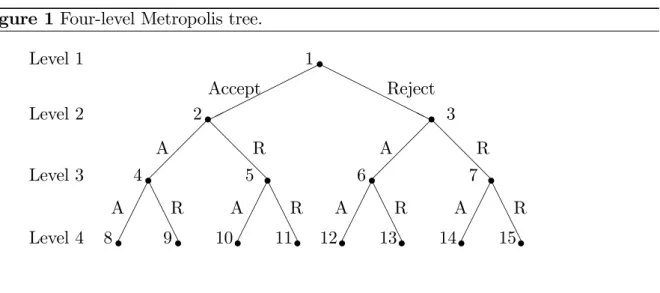
The prefetching algorithm can be pictured using a tree; here called a Metropolis tree (…gure 1). The nodes in the tree represent the possible future states of the chain. The number oflevelsof the tree,K, is related to the number of nodes,M;throughM = 2K 1.
The branches represent the decisions to accept or reject a proposal. Accepts are pictured as down-left movements and rejects as down-right movements in the tree.
Figure 1 Four-level Metropolis tree.
HH HH HHHH @ @ @ @ @ @ @ @ A A A A A A A A A A A A A A A A s 1 s 2 A R A R s 3 s 4 5 s 6 s 7 s s 8 A R A R A R A R s 9 10s 11s 12s 13s 14s 15s Accept Reject Level 1 Level 2 Level 3 Level 4
A node in the tree is associated with a state of the chain and a proposal based on this state. An evaluation of a proposed parameter will always occur at the start node i1 = 1. This corresponds to the evaluation required for a serial Metropolis-Hastings
algorithm. The state of the chain at node i1 is i, assuming that i draws have been
obtained previously, and the proposed parameter is 1 v f(:j i). If 1 is accepted the
chain moves from node 1 to node 2, with state i+1 =
1, and otherwise the chain moves
to node 3 and i+1 = i. More generally the states of the chain at nodes i
p and 2ip + 1
are the same whereas the proposed parameter is unique to each node.
The number of processes/processors (the terms are used interchangeably in this paper) is given by P. A description of the P nodes and the associated proposed parameters, at which the posterior is evaluated in parallel, is called a tour of sizeP
T (P) = fi1; i2; :::; iP; i1; i2; :::; iPg.
Often we refer to a tour merely by the node indices, assuming that it is understood how to determine the parameter points. The number of draws,D~(P; T), produced by a tour is a stochastic variable with support 1; :::; P. A chain consists of the draws obtained from a sequence of tours,fTng
N
n=1, and the last parameter reached by a tour becomes the starting
point for the next tour.
For an even node ip the parent node is i2p and for an odd node it is ip21. If a node
belongs to a tour, then its parent must also belong to the tour. The expected number of draws obtained from a tour of size P is denoted D(P; T) and it is given by
D(P; T) =
P
X
p=1
wherePr (ip)is the probability of reaching node ip and trivially Pr (1) = 1. The expected
number of draws of theoptimal tour, the tour that maximisesD(P; T)conditional on the branch probabilities in the Metropolis tree, is denoted D(P):
For some of the algorithms below the expected draws per tour can be obtained exactly whereas for others it is estimated via the average
d= 1 N N X n=1 dn, (2)
using the output of the Metropolis-Hastings prefetching algorithm, wherefdngNn=1 are the
realised number of draws from the tours fTngNn=1 and
d p!D,
by a law of large numbers. To obtain a chain of length R the required number of tours is N =ceil R=d and R~ =N P > R posterior evaluations occur in total. Thus R~ R of the posterior evaluations are useless.
Expected draws per tour, D(P), is equivalent to the theoretical speedup of the al-gorithm, i.e. it is the speedup in the absence of communication costs and other factors which a¤ect parallel e¢ ciency in practice. Draws per tour therefore provides an upper bound on the observed relative speedup
S(P) = T(1)
T(P), (3)
whereT(p)is the time of executing the parallel program usingpprocessors in a particular hardware and software environment. The di¤erence D(P) S(P) >0 thus depends on the precise nature of the parallel computing environment.
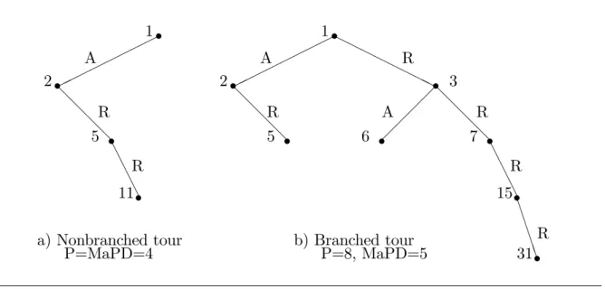
The maximum possible depth (MaPD) is the maximum number of draws that can be obtained from a tour, such that M aP D P. Also, let L = L(ip) be the function that
maps Metropolis tree indices to levels, e.g. L(7) = 3. A branched tour is a tour for whichM aP D < P. In other words it is a tour with the property that at least two nodes at the same level of the Metropolis tree are evaluated, i.e. L(ip) = L(ip~) for some pair
ip; ip~ 2 T. A nonbranched tour satis…es M aP D = P, or alternatively L(ip) = P for
exactly one ip 2T. The concepts are illustrated in …gure 2.
Astatic prefetching algorithm is an algorithm where all tours consist of the same nodes, i.e. the indices i1; :::; iP are constant across tours. For a dynamic prefetching algorithm,
on the other hand, the nodes of the tour vary as we move through the chain.
Parallel random number generation is not an issue in our context since naturally all random numbers are generated by one process. The random numbers should be generated such that the chain is independent of the number of processors used. If this is the case
Figure 2 Tours. @ @ @ @ A A A A s 1 s 2 R s 5 R s 11 A
a) Nonbranched tour b) Branched tour
P=MaPD=4 P=8, MaPD=5 HH HH HHHH @ @ @ @ @ @ @ @ A A A A B B B BB s 1 s 2 R R s 3 s 5 6 s A s 7 R s 15 A R s 31 R
not a¤ect the statistical properties of the chain. This is an implementational issue. The attachment of random numbers to draws implies that if tour n 1 produces dn 1 < P
draws then the random numbers attached to levels dn 1+ 1; :::; P of the Metropolis tree,
i.e. the levels that are not reached by the tour, should instead be used in tour n.
3.2
Examples
EXAMPLE 1 Assume that two processors,P1 and P2, are available for implementa-tion of the random walk Metropolis-Hastings (RWMH) algorithm. The …rst processor is necessarily employed for evaluation of the posterior kernel p at
1 = i+ i+1,
where i is the current state of the chain.
The second processor, P2, can be used either to prepare for an accept in the …rst stage, i.e. for evaluation of the posterior at
2 = 1+ i+2 = i+ i+1+ i+2,
or to prepare for a reject and evaluate the posterior at
3 = i+ i+2.
Assume that the acceptance probability can be chosen approximately as by proper selection of the increment densityg( ), e.g. by scaling the covariance matrix of a Normal
proposal density appropriately. Now, if < 0:5 it is obviously optimal to use P2 to prepare for a reject at the …rst stage (R1) and the optimal tour is T (2) =f1;3g.
If the …rst proposal is rejected two draws are obtained in one time unit using the two processors. If, on the other hand, 1 is accepted the posterior evaluation at 3 is useless.
In this case one draw is obtained in one time unit using two processors. The expected number of draws per time unit, or the theoretical speedup, is
D(2;f1;3g) = + 2 (1 ) = 2 .
This is an example of static prefetching since the tours that constitute the chain will contain the same node indices. It should also be noted that if instead >0:5the analysis is symmetric. In the remainder of the paper we restrict attention to the case < 0:5. The reason for this is our focus on the random walk variant of the Metropolis-Hastings method and it is further motivated by the discussion in section 3.3.5 below.
EXAMPLE 2 In the case of three processors,P1,P2andP3, assume <0:5as before. The optimal allocation of P1 and P2 is clearly the same as in the example above. For the third processor there are three options. First it can be employed for evaluation of
7 = i+ i+3,
i.e. anticipating rejects in the …rst two stages (R1,R2). A second possibility is to evaluate
2 in anticipation of an accept at the …rst stage. This yields the branched tour f1;2;3g
and D(3;f1;2;3g) = 2 draws are obtained with certainty, since P2 was used to prepare for a reject at the …rst stage.
The …nal possibility is to prepare for a reject in the …rst stage followed by an accept in the second stage (R1,A2) and evaluate
6 = i+ i+2+ i+3.
In the …rst case (R1,R2) the expected number of draws is
D(3;f1;3;7g) = + 2 (1 ) + 3 (1 )2. (4)
For example, with = 0:25this yields2:31. It is optimal to choose the nonbranched tour
f1;3;7g if D(3;f1;3;7g)> D(3;f1;2;3g) = 2, which is if 3 p5 2 0:38. Note that D(3;f1;3;7g) D(3;f1;3;6g) = (1 ) (1 2 )>0, for <0:5so it is never optimal to prepare for (R1,A2).
EXAMPLE 3 In the random walk Metropolis-Hastings algorithm a proposal at stage i + 1 is accepted with probability i+1 = min
fXi+1;1g, i.e. if ui+1 < Xi+1 for some ui+1 U[0;1]where
Xi+1 = p(
i+ i+1)
p( i) .
Consider example 1again and assume thatui+1 = 10 5 whereui+1 is the realised uniform
random number associated with draw i+ 1. Clearly, in this hypothetical situation it is wise to useP2to prepare for an accept, assuming no information about the posterior ratio Xi+1is available. The sequence of uniform random numbers,
fui
gRi=1 which are …xed from
the outset, thus carries some information on how to best structure prefetching.
EXAMPLE 4 The acceptance rate, ; and the sequence of uniform random numbers,
fui
gMi=1, can be used to improve the e¢ ciency of prefetching. Finally, knowledge about
the posterior, p, can be used to make better predictions on where the chain is moving. Assume that an approximation to the posterior, p , is available and that the evaluation of p takes a fraction of the time to evaluate p: Then this approximate distribution can be used to suggest the states which are likely to be visited subsequently.
In the limiting case when p =p we say that prefetching is perfect; it is analogous to importance sampling using the posterior as the importance function. In other words it is a situation when neither prefetching or importance sampling is necessary.
3.3
Algorithms
3.3.1 One-block random-walk Metropolis-Hastings prefetching
In this section the one-block Metropolis-Hastings prefetching algorithm is presented. This algorithm applies when all the parameters in are updated jointly and the proposal density f depends on the current state of the chain, e.g. for the one-block random walk Metropolis-Hastings sampler which we focus on here. It would be possible to use other proposal densities, e.g. a more general autoregressive proposal, but this route is not pursued here. Multiple block prefetching is discussed brie‡y at the end of this section and in appendix B.
The algorithm assumes that the posterior evaluation time is not parameter dependent and it is intended for application on a homogeneous cluster. The key assumption for application of the algorithm in practice is, loosely speaking, that the time of a posterior evaluation is signi…cant in relation to the other steps of the algorithm.
Algorithm 1 Metropolis-Hastings prefetching algorithm
1. Choose a starting value 0: Set the draw counter S 0 = 0.
2. (Prefetching step) Assume that the chain is in state Sn 1 when thenth tour begins,
where Sn 1 is the state of the draw counter aftern 1completed tours. Construct
a tour, Tn=fi1; :::; iP; i1; i2; :::; iPg(serial).
3. Distribute ip; p= 1; ::; P, to the processes (scatter).
4. Evaluatep ip in parallel.
5. Returnp ip (gather).
6. (Metropolis-Hastings step) Run the Metropolis-Hastings algorithm for the tourT to generateDn draws, where1 Dn P:Update the draw counter, Sn =Sn 1+Dn,
and assign the starting state for the next tour, Sn (serial).
7. Go to 2. Stop whenSn R draws from the posterior have been obtained.
The posterior evaluations, step 4 above, are performed in parallel. Communication between processes takes place in steps 3 and 5and message passing collective communi-cation tokens are used to describe the required operations. Steps 2 and 6 are performed by a master process or are replicated by all processors.
The Metropolis-Hastings step, step 6 in the above algorithm, is implemented in the following way for the random walk algorithm:
Algorithm 2 Random walk Metropolis-Hastings step
1. Set j = 1. The current state of the chain is Sn 1, where S
n 1 is the state of the
draw counter after n 1 completed tours. Let i1 = 1 be the proposal conditional
on the current state, i.e. 1 =f :j Sn 1 = Sn 1 + Sn 1+1.
2. The current node isip, with associated state Sn 1+j 1, and its level is L(ip) =j. If
uSn 1+j < Sn 1+j = min ( 1;p Sn 1+j 1+ Sn 1+j p( Sn 1+j 1) ) , (5)
whereu=U[0;1], accept the draw and set Sn 1+j = Sn 1+j 1+ Sn 1+j. Otherwise
set Sn 1+j = Sn 1+j 1.
3. If (i) the proposal ip =
Sn 1+j 1+ Sn 1+j was accepted and i
~
p = 2ip or (ii) if ip
was rejected and ip~= 2ip+ 1for some nodeip~2T then move to ip~. In this case set
The output from algorithm 2 are theDn draws from the tourn, Sn 1+1; :::; Sn; and
the output from the prefetching algorithm consists of the draws
Sn 1+1; :::; Sn N
n=1 =
1; 2; :::; SN ,
where N is the total number of completed tours and
N
X
n=1
Dn=SN R.
The remaining discussion in this section focuses on the prefetching step (step 2 of algorithm 1). The prefetching, or tour construction, problem consists of two separate parts:
1. Determine a rule for calculating the probabilities of reaching the nodes in the Metropolis tree based on some set of information.
2. Find the tour that maximises the expected number of draws per tour,D, based on these probabilities. We call this the optimal tour, with the implicit understanding that optimality is conditioned on the speci…c rule used.
The second task is easy and an algorithm which constructs the optimal tour given a rule for assigning the probabilities of the Metropolis tree is presented in appendix A. Below a parallel independence chain Metropolis-Hastings algorithm is …rst presented and then …ve variants of prefetching are discussed, named as follows: (1) Basic prefetching, (2) Static prefetching, (3) Dynamic prefetching using the sequence of uniform random numbers, (4) Dynamic prefetching using a posterior approximation and (5) Most likely path. Finally we discuss prefetching with multiple blocks and other proposal densities.
3.3.2 Independence chain Metropolis-Hastings
In the special case when the proposal density is …xed f j i =f( ),
parallelisation is simpli…ed further since there are no dependencies between posterior evaluations. Let R = P X p=1 Rp,
where Rp is the number of posterior evaluations performed by process p and R is the
Algorithm 3 Parallel Independence Chain Metropolis-Hastings (ICMH) algorithm
1. Each processp generates p = 1p; 2p; :::; Rpp where
ip f; i = 1; :::; Rp,
and collects the values of the posterior evaluated at these parameters in the vector pp = p( 1p); p( 2p); :::; p Rpp (parallel).
2. The master process gathers p and pp, p= 1; :::; P (gather).
3. Run the Metropolis-Hastings algorithm with the posterior already evaluated at R parameter values (serial).
In this algorithm the master process only collects the results from the other processes once. If memory limitation is a concern it can be solved by collecting the local results more often. In the case of inhomogeneous processors load balance is easily restored by allowing Rp to vary across processors.
The parallel ICMH algorithm is embarrassingly parallel both in the sense that it is simple to implement and because there is no essential dependency between the parallel tasks. As a consequence this algorithm will yield close to linear speedup, i.e. S(P) P, onany homogeneous parallel computer. The prefetching RWMH algorithm is also simple to implement but good parallel performance for this algorithm requires a balance between the problem (or problem size) and hardware/network since communication is frequent.
3.3.3 Basic prefetching
The basic prefetching algorithm suggested by Brockwell (2006) has the property that all future states at the same level in the Metropolis tree are treated as being equally likely to be reached. No information is used to structure prefetching. In our framework this algorithm is obtained if every branch in the Metropolis tree is assigned the probability
0:5.
The basic prefetching tour evaluates the proposed parameters of all nodes up to a given level of the Metropolis tree, i.e. T (P) =f1;2; :::; Pg, and thus produces a certain number of draws
D(P) = M aP D= log2(P + 1). (6) This approach provides a lower bound on the scalability that can be achieved using prefetching. Note that if the number of processors P does not correspond to the val-ues 2p 1; p = 1;2; ::: there is no clear guide on how to select the ‘surplus’ nodes for evaluation.
3.3.4 Static prefetching
The researcher can typically target an acceptance rate, , with good precision by selection of the proposal density, f, in the Metropolis-Hastings algorithm: Knowing it is easy to improve on the basic algorithm. Let T(Pj ;~) denote the tour when the acceptance rate is and the ‘perceived’acceptance rate used to construct the tour is ~, thus allowing for imperfect targeting. The static prefetching tour is obtained by attaching the probability ~
to all accept (down-left) branches of the Metropolis tree and 1 ~ to reject (down-right) branches. This was explained in some detail in examples 1 and 2 above for the cases P = 2and P = 3. The nonbranched tour shown in …gure 2 is obtained if we chooseP = 8
and target, for example, ~ = 0:25.
The node indices of the tours only needs to be obtained once per chain and the approach is general, i.e. model independent, since it only depends on the acceptance rate. For large enough and/or P the tour will be branched.
In …gure 3 the expected number of draws per tour,D( ; P), and the maximum possible depth (MaPD) of the optimal static prefetching tour is plotted against the acceptance rate
~ = 2 (0;0:5) for P = 3;7;15: The expected number of draws decreases smoothly in and above some threshold h(P) it becomes optimal to choose the basic prefetching
tour. If is below some threshold l(P)the optimal tour is nonbranched and an ‘always
prepare for a reject’ strategy is chosen. The MaPD curve jumps at points where the optimal tour changes.
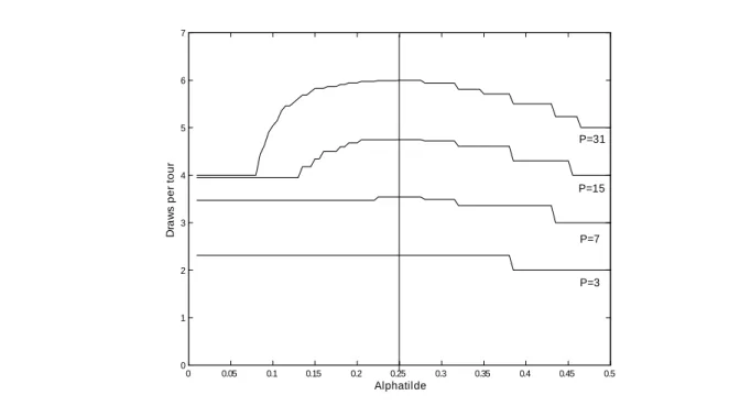
What happens if the tour is constructed based on a perceived acceptance rate ~ when the true acceptance rate is in fact ? In …gure 4 the expected number of draws is plotted for ~ 2(0;0:5) and P = 3;7;15;31 when the true acceptance rate is = 0:25. It is seen that it is optimal to use ~ = in constructing the tour but the optimal choice of ~ is not unique. For example, as was seen in example 2above, in the case of three processors any ~ 2 (0;0:38) will suggest the nonbranched tourT(3j0:25;~) = f1;3;7g which is the optimal tour if = 0:25:
3.3.5 Optimal static prefetching
A parallel e¢ ciency perspective obviously suggests targeting a low acceptance rate, as seen in …gure 3. Intuitively it becomes very easy to predict where the chain is moving when is small.
The optimal acceptance rate, opt;1 , for the random walk Metropolis-Hastings
algo-rithm has been derived under various assumptions on the target densityp(Roberts et al. (1997); Roberts and Rosenthal (2001)). Here we show how the optimal acceptance rate depends on the number of processors in a parallel computing framework, thus consid-ering jointly Markov chain, or statistical, e¢ ciency and parallel e¢ ciency of the static prefetching RWMH algorithm.
Figure 3 Static prefetching performance, ~ = . 0 0.05 0.1 0.15 0.2 0.25 0.3 0.35 0.4 0.45 0.5 0 2 4 6 8 10 12 14 16 Alpha D ra w s p e r to u r, M a P D P=3 P=7 P=15 MaPD, dashed Draws per tour, solid
Figure 4Static prefetching performance. The true acceptance rate is = 0:25and tours are constructed based on ~.
0 0.05 0.1 0.15 0.2 0.25 0.3 0.35 0.4 0.45 0.5 0 1 2 3 4 5 6 7 Alphatilde D raw s per t our P=7 P=15 P=31 P=3
We revisit the special case where the posterior density has the product form p( ) = k Y i=1 ~ p( k),
and the increment density, g, is of the form g( ) = N(0; Ik k2) where k2 = l2=k and
l is the scaling parameter. In the high-dimensional limit, i.e. as k ! 1, and under certain regularity conditions on p~it can be shown that the Markov chain converges to a di¤usion process and the optimal acceptance rate is obtained by maximising the ‘e¢ ciency function’
E1( )_ h 1 2
i2
, (7)
where is the standard normal cumulative distribution function. This yields the famous result of an optimal acceptance rate opt;1 = arg max E1( ) 0:234 (see Theorem 1 in
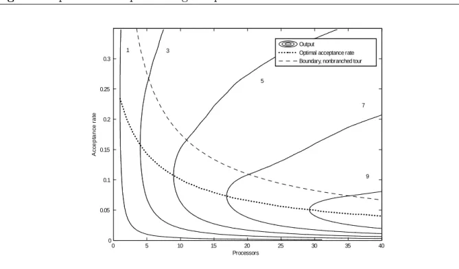
Roberts and Rosenthal (2001) and the subsequent discussion). In …gure 5 the joint output measure
E( ; P) =E1( ) D( ; P) c, (8) is plotted as a function of the acceptance rate and the number of processors P. The constant c is chosen such that E( opt;1;1) = 1. The …gure is interpreted as follows: the
time needed to achieve a given accuracy in estimating any function h( ) of the posterior is inversely related to the output E.
Theoptimal acceptance rate in a parallel setting is the acceptance rate which minimises the time of obtaining a sample of a …xed size and quality, e.g. a …xed number of iid draws, from the posterior, conditional on the number of processors used. It is seen in …gure 5 that the optimal acceptance rate implies an ‘always prepare for a reject’prefetching strategy. The optimal rate is below the nonbranched tour boundary which is de…ned implicitly by = (1 )P 1: For example, using P = 7 processors the optimal acceptance rate is opt;7 = 0:120 and a sample of a given size and quality from the posterior can be
obtainedE( opt;7;7) = 4:3times faster than when applying one processor and the optimal
acceptance rate opt;1 = 0:234:
Our choice of cimplies that E( opt;P; P) is interpreted as the optimal speedup of the
static prefetching RWMH algorithm and it satis…es
D( opt;1; P) E( opt;P; P) D( opt;P; P),
where equality holds for P = 1. For the case of P = 7 processors we haveE( opt;1;7) =
D( opt;1;7) = 3:65. The bene…t of lowering the acceptance rate from opt;1 = 0:234 to
opt;7 = 0:120, the gain in parallel e¢ ciency, is larger than the cost, the loss of statistical
Figure 5 Optimal static prefetching acceptance rates. Processors Ac c ept anc e r at e 0 5 10 15 20 25 30 35 40 0 0.05 0.1 0.15 0.2 0.25 0.3 Output
Optimal acceptance rate Boundary, nonbranched tour
9 3
1
7 5
More generally the optimal acceptance rate opt;P will be determined by the curvature
of the e¢ ciency functionE1( ). In a serial computing setting a ‡at e¢ ciency curve implies that it is ‘of little value to …nely tune algorithms to the exact optimal values’(Roberts and Rosenthal (2001)). In a parallel computing setting the implication is that parallel e¢ ciency can be improved, by lowering the acceptance rate, without incurring a large cost in terms of statistical e¢ ciency.
In our applications below the e¢ ciency function E1( ) is not available analytically
and hence the optimal acceptance rate opt;P cannot be solved for. Instead we target an
acceptance rate = 0:25 for allP, a ‘conservative’choice, and compare the parallel e¢ -ciency of di¤erent prefetching approaches while keeping the statistical properties …xed. In the main illustration the empirical static prefetching optimal speedup and the associated empirical optimal acceptance rates are also obtained.
Finally, in the processor limit
lim
P !1 n
arg maxE( ; P)o= lim
P !1 opt;P = 0.
In other words we can a¤ord to make the algorithm arbitrarily poor, in the statistical sense, only if parallel computing technology is arbitrarily cheap.
3.3.6 Dynamic prefetching based on the uniform random numbers
The probability of accepting a proposal z drawn from f( j i) depends on the realised
value of a uniform random number, ui+1. Let Xi+1 = p( z)
p( i),
and consider the conditional acceptance probability
i+1
ui+1 = Pr ui+1 < Xi+1jui+1 ,
where u is treated as …xed and X as stochastic. Since it is possible to characterise the relationship between and u the static prefetching algorithm can be improved upon.
In the applications below we incorporate information from the sequence of realised uni-form random numbers in the following way. First R draws from the Metropolis-Hastings sampler are obtained. Next, the unit interval is divided into K subintervals Ik and an
empirical acceptance rate
k =
#ffu < Xg \ fu2Ikgg
#fu2Ikg
, (9)
is calculated for each subinterval k = 1; :::; K based on approximately R=K draws. The constant acceptance rate used in the static prefetching algorithm above is then replaced by an acceptance probability which depends on a uniform random number
i+1 ui+1 = K X k=1 kI ui+1 2Ik , (10) whereIk = [ (k 1) K ; k
K]andI is the indicator function. This algorithm has the property that
the branch probabilities in the Metropolis tree are level-speci…c, i.e. all accept branches at the same level in the tree will have the same probability attached to them.
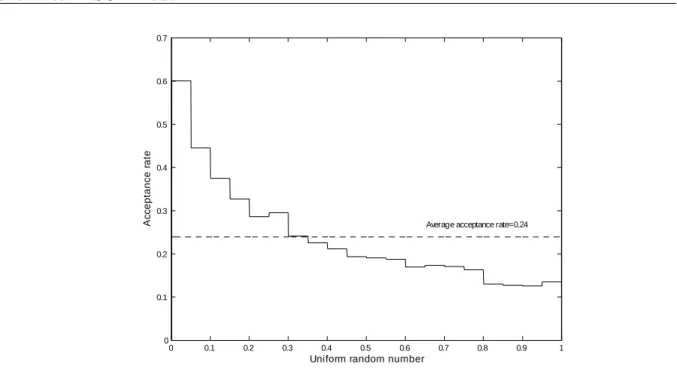
The procedure is illustrated in …gure 6 where the acceptance rate is plotted against the uniform random number for the linear estimation example presented later in the paper. HereR = 100;000draws are used to obtain estimates of kforK = 20equally sized
subin-tervals. For example it is seen that 1 = 0:60 is the estimate ofPr (u < Xju2[0;0:05]):
3.3.7 Dynamic prefetching based on a posterior approximation
If a posterior approximation, p , is available and if evaluation of p is fast in comparison with the posterior kernel p a possibility is to use p to determine at which parameters to evaluate p. The objective is thus the same as in importance sampling or indepen-dence chain Metropolis-Hastings (ICMH) sampling, i.e. to …nd a good approximation
Figure 6 Acceptance rate as a function of the uniform random number in the estimation of a linear DSGE model.
0 0.1 0.2 0.3 0.4 0.5 0.6 0.7 0.8 0.9 1 0 0.1 0.2 0.3 0.4 0.5 0.6 0.7
Uniform random number
Ac
c
eptanc
e r
ate
Average acceptance rate=0.24
to the posterior. However, a di¤erence is that the quality of the approximating density used for prefetching has no implications for the statistical analysis; it will ‘merely’a¤ect computational e¢ ciency.
For the RWMH algorithm one possible strategy is to simply replace the constant in the construction of the static prefetching tour with the probability
min ( ;p ip p ( i) ) , where ip =
i+ and thus incorporate information about the posterior in the construction
of the tour. We call this dynamic prefetching using a posterior approximation. If < 1
then Pr (ip)>0 for allp, i.e. all nodes of the Metropolis tree have positive probability of
being visited. In the application below we let = 1, thus eliminating parts of the tree. As in the static prefetching case the tour will in general be branched.
Another possibility is to run the chain P steps ahead using the approximate density, thereby also incorporating the information contained in the sequence of realised uniform random numbers. The states visited using the approximate posterior yield the parame-ter points at which the posparame-terior p is subsequently evaluated in parallel. The tour is nonbranched and we call this type of algorithm a most likely path algorithm.
3.4
Marginalisation and blocking
The Dynamic Stochastic General Equilibrium (DSGE) models used for the illustrations in this paper are represented as state-space models. The coe¢ cients of the DSGE-state-space model are nonlinear functions of the structural parameters, . The latent variables, collected inx, are integrated out of the joint posteriorp( ; xjy)using …ltering techniques and attention is restricted to the marginal posterior density, p( jy), where y denotes the data. Sampling from the conditionalp( jx; y)is precluded for these models. In the main example, in section 4.1, the Kalman …lter is applied for integration in a degenerate linear and Gaussian state-space (LGSS) model. If there is interest in the posterior distribution for the state variables, p(xjy), this distribution is obtained via smoothing after p( jy)
has been sampled, see e.g. Durbin and Koopman (2001). The marginalisation technique has also been used in other contexts, e.g. Garside and Wilkinson (2004).
For comparison, consider the more typical LGSS model where interest centers on p( ; xjy)and where, in contrast to the linearised DSGE model, the classic two-block data augmentation scheme is available. The conditional posterior p( jx; y) is sampled using Gibbs or Metropolis updates and p(xj ; y) is sampled using a simulation smoother, e.g. Strickland et al. (2009). A Gibbs step, viewed as a Metropolis-Hastings update with ac-ceptance probability 1, implies perfect prefetching and hence prefetching does not apply. In situations where a Metropolis-Hastings block sampler with reasonably good mixing properties is available we expect prefetching to be of limited use and, if thought neces-sary, other parallelisation approaches should be considered. Wilkinson (2006) shows how to exploit the conditional independence structure to parallelise the multimove simulation smoother used for estimation of the baseline stochastic volatility (SV) model. This ap-proach can also be applied to extended SV models and the stochastic conditional duration (SCD) model, for which e¢ cient block sampling schemes have been developed (Omori and Watanabe (2008); Takahashi et al. (2009); Strickland et al. (2006)). A similar ‘parallel blocks’approach is also applied by Whiley and Wilson (2004).
There are two features, in addition to the inability to sample from p( jx; y), which increase the attractiveness of the one-block prefetching approach for DSGE models. First, it is typically a nontrivial task, at leasta priori, to split the parameter vector into blocks such that there is weak posterior dependency between blocks. Second, the resulting Metropolis sampler with B blocks is ‘penalised’by a B-factor increase in computational time relative to the one-block sampler.
More generally, although prefetching generalises to the case of Metropolis multiple block sampling parallel e¢ ciency is expected to su¤er in that context, at least when a subset of the full conditionals can be sampled directly. If high dimensionality of the parameter vector, rather than exploitable structure, is the motive for splitting the para-meters into blocks then Metropolis block prefetching could be interesting but this is not investigated further here. A brief description of block prefetching is given in appendix B. Another potentially interesting application for prefetching methods, not fully explored
in this paper, is the class of hierarchical Gaussian Markov random …eld (GMRF) models with a wide range of applications, e.g. in spatial statistics (Knorr-Held and Rue (2005)). Knorr-Held and Rue (2002) develop a ‘hyperblock’sampler for this type of model, using the methods for fast sampling from GMRFs presented by Rue (2001). This is another, more elaborate, example of a marginal updating scheme where the hyperparameters and the latent …eld x are updated jointly using a Metropolis-Hastings step.
Knorr-Held and Rue (2002) demonstrate that the hyperblock sampler mixes more rapidly than the traditional single-site updating scheme and various intermediate blocking schemes in three typical disease mapping applications. The results are driven by the strong posterior dependency between and xin these applications. A one-block sampler for linear mixed regression models, along similar lines, is suggested by Chib and Carlin (1999). The marginalisation approach is also used by Gamerman et al. (2003) for spatial regression models and in Moreira and Gamerman (2002) for time series models.
The possibility of prefetching parallelisation may be interpreted as a further argument in favour of the sophisticated one-block sampling scheme for GMRF models, in addition to the documented improvement in chain mixing. In fact, the ‘always prepare for a reject’ prefetching strategy applies to a more general one-block sampler, suggested by Wilkinson and Yeung (2004) for the related class of linear Gaussian Directed Acyclic Graph (DAG) models. In appendix B we outline how to apply prefetching in the GMRF context and also mention the possibility of combining prefetching with the parallel GMRF sampling approach suggested by Steinsland (2007).
4
Illustrations
4.1
Linear estimation of a DSGE model
Long burn-in times and poor mixing are factors that can motivate interest in single-chain parallel methods. In the area of Bayesian estimation of Dynamic Stochastic General Equilibrium (DSGE) models the one-block random walk Metropolis-Hastings algorithm is the most commonly used estimation method and our impression is that poor mixing of chains is a typical experience of researchers in this …eld. For an exception, see Belaygorod and Dueker (2006).
The performance of the …ve variants of the prefetching algorithm presented above and the parallel ICMH algorithm is compared using one of the core macroeconomic models at the European Central Bank, the Smets and Wouters (SW) model (Smets and Wouters (2003)). The model is chosen because it is well known and since it is the backbone of larger DSGE models currently developed at many central banks. A major determinant of the computational cost of estimating a DSGE model is the number of state variables of the model. Our version of the SW model has15state variables, including 8shocks. Recently developed large-scale microfounded models in use at central banks have as many as 65
state variables and there is at least one very recent example of a model which contains more than 100 state variables (Adolfson, Laséen, Lindé and Villani (2007); Christiano et al. (2007)). In a relative sense, and using the jargon of parallel computing, this implies that our estimation problem can be viewed as …ne-grained.
The empirical analysis of large-scale DSGE models is restricted by the computational cost of estimating them. Re-estimation is necessary as di¤erent model speci…cations are evaluated or when new data arrives. Furthermore, a central bank is facing real-time constraints on these activities. In our view the development of larger and more complex models and the unavailability of adequately e¢ cient sampling methods increase the attractiveness of applying the parallel methods presented here.
4.1.1 Model, prior, solution and likelihood
The economic content of the model is largely unimportant for our evaluation of the parallel algorithms and therefore it is not presented here. Similar models have been analysed and/or estimated in many articles (Smets and Wouters (2003); del Negro et al. (2005)). The model used here is presented in detail in Strid (2007a).
The model consists of a set of nonlinear expectational equations describing the equi-librium and a linear approximation to the policy function of the model is obtained (the solution). The linear approximate policy function is represented as a linear state-space model:
Xt=T( )Xt 1+R( ) t (11)
and
Yt =d( ) +ZXt+vt, (12)
where [11] is the state equation and [12] the measurement equation. Here Xt (dimension
nx) is a vector containing the state variables andYt(ny) is a vector containing the observed
variables. The structural parameters of the model are collected in the vector (n ) and the coe¢ cient matrices, T (which is dense), R and Z, and the vector d are nonlinear functions of . The innovations, t (n ), and the measurement errors,vt(nv), are assumed
to be independent and normally distributed, tvN(0; ) and vt vN(0; v).
The likelihood evaluation consists of two parts. First the model is solved using one of the many available methods (Klein (2000)). Second the likelihood function of the model is evaluated using the Kalman …lter, see e.g. Durbin and Koopman (2001). The prior distribution for is similar to the distributions typically used in the literature on estimation of New Keynesian models.
For the model estimated here we have the dimensions nx = 15; ny = 5; n = 8 and
n = 23. The model is estimated on Euro Area data for the period 1982:1-2003:4 (88
observations). The …ve data series used for estimation are the short-term interest rate, in‡ation, output growth, the consumption-to-output ratio and the investment-to-output ratio.
4.1.2 Parallel approaches for linearised DSGE models
In the context of estimation of large-scale linearised DSGE models, what other strate-gies for single-chain parallelisation are available apart from prefetching? An obvious within-draw approach is to apply parallel matrix algorithms (e.g. using ScaLAPACK or PLAPACK) to the computations involved in Kalman …ltering, primarily the matrix multiplications of the Riccati equation which account for a signi…cant part of Kalman …ltering time. However, if this approach is attempted it is crucial to apply parallel rou-tines whenever fruitful, including in the solution algorithm. The extent to which a few standard matrix operations account for overall Kalman …ltering and model solution time determines the parallel e¢ ciency properties of the approach. Furthermore, it is hard to improve on optimal serial DSGE-speci…c Kalman …lter implementations using parallel methods, see Strid and Walentin (2008).
Note again that it would be straightforward, at least in principle, to combine such local computations strategies, which are somewhat more demanding to implement, with prefetching.
4.1.3 Parallel e¢ ciency: draws per tour
The posterior approximation used for prefetching (variants 4 and 5) is a normal approx-imation p = N( m; m) where m is the posterior mode, Hm the Hessian matrix at the
mode and m=Hm1. The scaled inverse Hessian is also used as the covariance matrix for
the proposal density in the random walk Metropolis-Hastings algorithm, i.e. proposals are generated with
z = i+ i+1,
where i+1 N(0; cH 1
m ) and cis a scaling parameter.
Prior to optimisation of the posterior p and estimation using the RWMH algorithm some parameters in are reparameterised to make the parameter space unbounded. The reparameterisation serves two purposes: …rst, it makes optimisation easier and, second, the e¢ ciency of sampling using the RWMH algorithm is improved because the approxi-mation to normality is better. In the context of prefetching the reparameterisation will thus also improve the parallel e¢ ciency of the algorithms which rely on the posterior approximation.
For each combination of prefetching algorithm and number of processorsP the RWMH prefetching algorithm is used to sample R = 500;000 draws from the posterior distribu-tion. In total the posterior is evaluated R~ = N P =RP=d times where N is the number of tours and d is the average number of draws per tour. In all estimations the chain is started at the posterior mode and50;000 draws are discarded as burn-in. A target accep-tance rate ~ = 0:25 is used to construct the tours in static prefetching (2) and dynamic prefetching based on the uniform random numbers (3) and the average acceptance rate
Table 1 Performance of prefetching algorithms for the linearised DSGE model. Average number of draws per tour, d.
Processors
Algorithm variant 1 3 7 15 31 1
1. Basic prefetching 1 2 3 4 5 1
2. Static prefetching 1 2.31 3.54 4.75 6.00 1 3. Dynamic prefetching, uniform 1 2.38 3.81 5.04 6.24 1 4. Dynamic prefetching, post. approx. 1 2.57 4.58 6.45 8.04 -5. Most likely path 1 2.66 4.99 7.31 8.42 8.70 6. Optimal static prefetching speedup 1 2.44 4.30 6.55 6.55
-Optimal empirical acceptance rate 0.22 0.16 0.13 0.09 0.05
algorithm. Detailed results on prefetching performance are presented for P = 2p 1; p = 1; :::;5. These values are chosen because they allow for a neat comparison with the benchmark basic prefetching algorithm, which has integer draws per tour for these values of P (see expression [6]).
In table 1 the average number of draws per tourd are presented. It is seen, …rst, that static prefetching allows us to make easily reaped, although quite small, gains in compar-ison with the basic algorithm. Second, incorporating knowledge about the sequence of uniform random numbers lead to additional small gains. These e¢ ciency improvements are model independent and can always be obtained.
Third, in our example the inclusion of information about the posterior via the normal approximation yields the largest gains. For example, using the most likely path algorithm (5) withP = 7processors the extra draws, i.e. the draws which are added to the sure draw, is doubled in comparison with the basic algorithm (1). If a reasonable approximation to the posterior is available it thus appears possible to improve the parallel e¢ ciency of prefetching quite substantially.
Finally, we report empirical measures of the static prefetching optimal speedup and optimal acceptance rates for this problem (6). Note that these quantities are adjusted for di¤erences in sampling e¢ ciency when targeting di¤erent acceptance rates. Thus direct comparison with the other approaches is possible. The experiments conducted to obtain these numbers are described in appendix A. Also note that we have not been able to increase the quality-adjusted speedup for the most likely path algorithm (5) by targeting lower acceptance rates in this way.
The results reported above must be interpreted with caution. If the parallel perfor-mance of the most likely path algorithm is becoming ‘too good’ it suggests that other approaches, such as independence chain Metropolis-Hastings (ICMH), should be consid-ered. For our estimation problem we have veri…ed that the sampling e¢ ciency of ICMH using standard choices of proposal densities, e.g. the multivariatet, is inferior to the e¢ -ciency of RWMH. The acceptance rate of the best ICMH sampler is13%. If the thinning
factor for ICMH is roughly eight times the factor used with the RWMH sampler it is found that the relative numerical e¢ ciencies, or the ine¢ ciency factors, of the two approaches are roughly similar.
4.1.4 Parallel e¢ ciency on an HPC cluster
Draws per tour, D(P);is an abstract measure of scalability since the cost of constructing tours and communication cost is not taken into account. In order to assess the magnitude of the di¤erence between theoretical and actual speedup, D(P) S(P), the algorithms are taken to a parallel computer. The prefetching algorithm is implemented using Fortran and the Message Passing Interface (MPI) and tested on the Lenngren cluster at the Center for Parallel Computers (PDC) at the Royal Institute of Technology (KTH) in Stockholm, a high performance computing (HPC) environment. The cluster uses Intel Xeon 3.4GHz processors connected by an In…niband 1GB network. The MPI implementation on the cluster is Scali MPI. Further information on the performance characteristics of the cluster is available at www.pdc.kth.se.
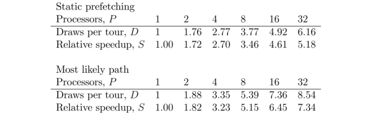
For each combination of P and algorithm an acceptance rate ~ = 0:25 is targeted and R = 500;000 draws from the posterior are obtained. In table 2 the draws per tour D and relative speedup S, as de…ned in [3], are reported for P = 2p; p = 0; ::;5 for the
static prefetching algorithm (2) and the best performing algorithm according to table 1, the most likely path algorithm(5). Using one processorR= 500;000 draws are obtained in80minutes and using P = 8 processors the static prefetching algorithm (2) executes in
23 minutes and the most likely path algorithm (5) in15minutes.
It is seen that for the particular model, programming language, implementation and hardware the speedup is acceptably close to the upper bound, at least for P = 1 8. We conclude that on a representative HPC cluster the RWMH prefetching algorithm can be implemented successfully for a …ne-grained problem. For the large-scale models mentioned above we expect S D in this environment.
4.1.5 Discussion
In an article written by researchers at the Riksbank, the central bank of Sweden, some econometric issues related to the estimation of a large-scale linearised open economy DSGE model (the RAMSES model) are addressed (Adolfson, Lindé and Villani (2007)). We present some of their observations because we believe they are representative to this …eld of research:
1. Computing time is a major concern when Bayesian methods are employed to analyse large-scale DSGE models.
Table 2 Performance of prefetching algorithms for the linearised DSGE model on the Lenngren cluster.
Static prefetching
Processors,P 1 2 4 8 16 32
Draws per tour,D 1 1:76 2:77 3:77 4:92 6:16
Relative speedup,S 1:00 1:72 2:70 3:46 4:61 5:18
Most likely path
Processors,P 1 2 4 8 16 32
Draws per tour,D 1 1:88 3:35 5:39 7:36 8:54
Relative speedup,S 1:00 1:82 3:23 5:15 6:45 7:34
ICHM algorithm is that it easily gets stuck for long spells when the parameter space is high-dimensional.
3. Blocking approaches are di¢ cult to implement for these models because full condi-tional posteriors are not easy to simulate from. Furthermore, this approach requires multiple evaluations of the likelihood per posterior draw.
4. It is found for the RWMH algorithm that decreasing the targeted acceptance rate from 0:25 to0:10leaves the ine¢ ciency factors largely unaltered.
5. Reparameterisation increases the e¢ ciency of sampling substantially.
These observations are largely con…rmed by our exercise above and taken together we believe that they increase the attractiveness of prefetching methods in the context of large-scale linearised DSGE models.
Computing time The issue of when computing time becomes a real concern is largely context-speci…c. Clearly in our environment, characterised by a relatively small DSGE model, Fortran code and decent computing power, the rationale for parallel methods is perhaps limited, as indicated by the absolute execution times reported. Even for a model of this size it is however clear that the scope of experiments that can be performed in a given time span is increased.
In a more typical desktop computing environment, and using state-of-the-art DSGE modelling tools like DYNARE or YADA, single runs may take several days for the most re-cent generation of policy-relevant DSGE models. Total project computing time, including a substantial amount of experimentation, is measured in months.
RWMH vs. ICMH The parallel e¢ ciency of ICMH is far superior to that of RWMH. Using ICMH with P = 64 processors to generate one million draws from the posterior distribution of the SW model the total execution time is around 2:5 minutes on the Lenngren cluster and the relative speedup isS(64) = 63. Although the ICMH sampler has much to recommend to it, especially in a parallel setting, in our example problem it does not seem straightforward to …nd an e¢ cient proposal density. In a serial programming context the choice of estimation strategy would certainly be to use the RWMH algorithm. In a parallel framework the trade-o¤s are slightly more complicated and several factors must be taken into account.
The following example clari…es the trade-o¤s for our example under the assumption that ICMH requires a thinning factor which is 8times that of RWMH to achieve roughly the same sampling e¢ ciency. If P = 128 processors are used to estimate the model above with the two algorithms, parallel ICMH and RWMH prefetching, then a posterior sample of a given quality, as judged by the ine¢ ciency factor, can be obtained roughly twice as fast for the ICMH algorithm in comparison with prefetching. IfP = 8processors are used the execution time of prefetching is more than 5 times faster than for parallel ICMH.
Acceptance rate The fourth observation above is especially interesting in relation to prefetching. As demonstrated above the empirical optimal static prefetching e¢ ciency is not far behind the e¢ ciency of the most likely path approach for the relevant range of processors in our problem. These two approaches are also the simplest to implement, since they imply nonbranched tours.
To conclude a simple heuristic strategy is suggested: choose the scaling of the incre-mental density to obtain the optimal static prefetching acceptance rate conditional on the number of processors (see …gure 5) and use the ‘always prepare for a reject ’tour. It can be expected that often this will be reasonably close to the optimal overall prefetching strategy.
4.2
Nonlinear estimation of a DSGE model
In this section the Metropolis-Hastings prefetching algorithm is applied to the problem of estimating a nonlinearly approximated small-scale DSGE model using Bayesian methods. In the previous section we established that in a high performance computing (HPC) envi-ronment, i.e. on the Lenngren cluster, the prefetching algorithm works successfully for a …ne-grained estimation problem. Our main objective in this section is to assess prefetching performance in a particular personal high performance computing (PHPC) environment: using the parallelism of Matlab (the Distributed Computing Toolbox, DCT) on a quad-core desktop computer. Alternatively, and perhaps more correctly, we may interpret this exercise as an evaluation of the parallel functionality of Matlab, using the prefetching algorithm as the test ground. The multi-core/Matlab environment is presumably one of
The nonlinear estimation example is chosen …rst because it is an estimation problem that should be su¢ ciently coarse-grained to deliver reasonable parallel e¢ ciency also in the PHPC environment. Note that for a given model the particle …lter based evaluation of the likelihood for the quadratically estimated model is roughly1000times slower than the Kalman …lter likelihood evaluation for the corresponding linearly approximated model. Second, the discontinuous likelihood approximation in the nonlinear case implies that prefetching methods which rely on a posterior approximation (variants 4 and 5 above) cannot be implemented without modi…cation. In other words, the most successful variants of prefetching in the linear estimation example of the previous section are not readily available to us here.
4.2.1 Model, prior, solution and likelihood
The prototypical small-scale New Keynesian model is borrowed from An (2005). Again, the economic content of the model is largely irrelevant for our purposes here and therefore no discussion of the model is provided.
The policy function of the model is approximated to the second order using the ap-proach of Schmitt-Grohe and Uribe (2004). The approximative solution can be cast in the following state-space form. The state equation is separated into an equation for the exogenous state variables (the shocks)
X1t=AX1t 1+"t, (13)
and an equation for the endogenous predetermined variables and a subset of the nonpre-determined variables
X2t=BX~t 1+Cvech( ~Xt 1X~tT 1) +e, (14)
where X~t 1 = X1Tt X2Tt 1 T and Xt= X1Tt X2Tt T.
In this way a linear observation equation,
Yt=d+ZXt+vt, (15)
is obtained. The innovations and measurement errors are assumed to be independent and normally distributed, "t N(0; Q) and vt N(0; H): The second order policy
function approximation of a large class of DSGE models can be cast in this form. The state-space representation of the corresponding linearly approximated model, which was used in the previous example, is obtained by letting C = 0 and e = 0. The matrices A( 2); B( 1); andC( 1) and the vectorse( ) and d( 1)are functions of the parameters
of the economic model, which are collected in = T1 2T T where 1 consists of the
structural parameters of the model and 2 contains the auxiliary parameters, i.e. the
parameters describing the shock processes. The dimensions of the vectors are nx1 = 3;
The model is estimated on simulated data and we use the same data-generating process, dgp, as An (2005) and a prior distribution for similar to the one in An’s
paper. The likelihood function of the model is evaluated using an Adaptive Linear Par-ticle Filter (ALPF), designed for the particular state-space model described by equations [13]-[15] [Strid (2007a)]. The particle …lter and its application to the nonlinear estimation of DSGE models is not discussed in detail here and the reader is referred to the refer-enced articles (Arulampalam et al. (2002); Doucet et al. (2000); Fernández-Villaverde and Rubio-Ramírez (2007); Amisano and Tristani (2007)).
4.2.2 Implementation
The estimation routine is implemented in Matlab, using a Fortran mex function only for the systematic resampling (SR) step of the Adaptive Linear Particle Filter. The SR algo-rithm cannot be implemented as vectorised code, implying that a Fortran implementation of this part of the particle …lter is considerably faster than its Matlab counterpart. The likelihood evaluation accuracy of the ALPF …lter applied here is at least as good as for a standard particle …lter with 40;000 particles and the time of a posterior evaluation is roughly 2:5s for this Matlab implementation.
The parallel section of the prefetching algorithm, step 4 of algorithm 1, is implemented using the parallel for-loop (parfor) construct contained in the Parallel Computing Toolbox. The number of calls to parfor is thus equal to the total number of tours, N.
4.2.3 Experiment
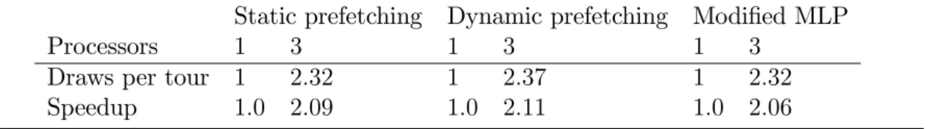
The Metropolis-Hastings prefetching algorithm is executed on an Opteron 275, 2.2 Ghz, using three of the four available cores. Three variants of prefetching are tested: (i) static prefetching, (ii) dynamic prefetching based on the uniform random numbers and (iii) a modi…ed most likely path (MLP) algorithm. The modi…cation of the MLP algorithm in (iii) consists of updating the mode of the normal approximation to the posterior in order to obtain a successively better approximation, even though the exact mode cannot be obtained. This type of adaptation only a¤ects the quality of prefetching and not the statistical properties of the chain. The starting mode of the approximation is the linear posterior mode.
An acceptance rate ~ = 0:25 is targeted and the actual rate is 0:24. The potential suboptimality of this choice for P = 3 is disregarded. In each case 50;000 draws from the posterior are obtained. Draws per tour and speedup are presented in Table 3. First, the problem is su¢ ciently coarse-grained for implementation in the particular PHPC environment, in the sense that absolute speedup is acceptably close to draws per tour. Second, the results suggest that it is hard to improve on static prefetching when a good posterior approximation is not immediately available. All three variants roughly halves estimation time when three cores are used, from 35to17 hours of computing time.
Table 3Performance of prefetching algorithms for the nonlinear DSGE model in a multi-core/Matlab environment.
Static prefetching Dynamic prefetching Modi…ed MLP
Processors 1 3 1 3 1 3
Draws per tour 1 2:32 1 2:37 1 2:32
Speedup 1:0 2:09 1:0 2:11 1:0 2:06
5
Two-layer parallelism
In this section we brie‡y discuss the possibility of either (i) combining prefetching with lower level parallelism or (ii) using prefetching performance to evaluate competing parallel algorithms. In the context of the Metropolis-Hastings algorithm lower level, and hence competing, parallelisation means any type of within-draw parallelisation of the posterior evaluation. Since prefetching is a general, i.e. largely problem independent, single-chain parallel algorithm it can be used to suggest admissible regions for the number of processors used by the lower level parallel algorithm. Competing parallel algorithms are necessar-ily problem-speci…c, presumably more complicated both to develop and implement and they certainly require more frequent communication between processors. This suggests a natural benchmark role for the prefetching algorithm.
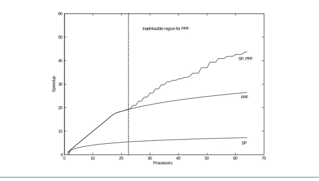
The potential performance gain of combining prefetching with a lower level parallel algorithm is illustrated using the nonlinear estimation example considered above. A Par-allel Standard Particle Filter (PPF) is used for the likelihood evaluation. The speedup numbers for the PPF refer to Fortran/MPI implementations run on the Lenngren clus-ter (Strid (2007b)). The number of particles employed is N = 40;000. For the static prefetching (SP) algorithm an acceptance rate of = 0:25is targeted.
In …gure 7 it is seen that the PPF is much more e¢ cient than the prefetching approach. (The kink in speedup for the PPF is explained by the fact that we estimate a speedup function based on a set of observations S(P); P = 1;2;4; :::;64 ; while ruling out the possibility of superlinear speedup.) However, when the number of processors exceedPopt = 22it becomes optimal to switch to the two-layer parallel algorithm which combines static prefetching with the PPF. As the number of processors increase the speedup di¤erence between the two-layer algorithm and the PPF becomes quite pronounced. It is also possible that a minor improvement in speedup, adjusted for statistical e¢ ciency, can be achieved by targeting a lower acceptance rate for prefetching.
The simple calculations underlying …gure 7 show how consideration of the prefetching alternative can guide decisions on the tolerable number of processors to use for the lower level parallel algorithm for a given estimation problem and problem size (here the number of particles employed in the particle …lter). Importantly this type of scalability analysis can be performed without ever implementing the prefetching algorithm.
Figure 7Two-layer parallel performance. Static prefetching and a parallel particle …lter applied for the estimation of a nonlinear DSGE model.
0 10 20 30 40 50 60 70 0 10 20 30 40 50 60 Processors S p ee dup SP PPF SP, PPF Inadmissible region for PPF
6
Conclusions
Prefetching algorithms have obvious limitations in terms of parallel e¢ ciency. This is due to the inherently sequential nature of the Metropolis-Hastings algorithm. The advantages of the independence chain Metropolis-Hastings algorithm in a parallel context are obvious. In this paper we have shown how to substantially increase the e¢ ciency of prefetching using some simple techniques. Even using these techniques on reasonably well-behaved, unimodal, problems it is hard to imagine anyone applying more than, say,10 15 proces-sors to a prefetching algorithm. Despite this the simplicity of implementing the method and the possibility of a multiplication e¤ect if combined with lower level parallelisation were claimed to motivate interest in the method.
The paper has highlighted some complicated trade-o¤s. First, for the prefetching algorithm a parallel e¢ ciency perspective suggests targeting of a low acceptance rate. This must be weighted against Markov chain e¢ ciency considerations. For the random walk Metropolis-Hastings algorithm it was demonstrated that the optimal acceptance rate decreases with the number of processors applied to the algorithm. Second, ‘good’ scalability of prefetching when a posterior approximation is used to construct tours may indicate that other sampling approaches should also be considered.
Bayesian estimation of DSGE models was identi…ed as one potential arena for prefetch-ing methods. In this context the experiences reported by researchers at the Riksbank,
which largely correspond to the results reported here for a smaller model, suggest that prefetching methods is a viable alternative in reducing estimation time. The generality of the proposed method, however, suggests that it could be applied in other contexts as well. Brockwell (2006) applies prefetching to long memory time series models. The application of prefetching with the hyperblock sampling approach for GMRF models and in related contexts should be more thoroughly explored in future research.
Finally, it would be straightforward to implement a prefetching version of the adaptive RWMH algorithm proposed by Haario et al. (2001). In many cases we expect the proposal distribution of the RWMH and the posterior approximation used to make prefetching pre-dictions to coincide, possibly with a di¤erent scaling as in our linear estimation example. The adaptive RWMH can then potentially increase statistical and parallel e¢ ciency si-multaneously.
Appendix A
The prefetching algorithm
Let L = L(ip) be the function that maps Metropolis tree node indices to levels, e.g.
L(10) = 4:The expected number of draws D(P)for the tour T(P) =fi1; :::; iPg is given
by D(P) = P X p=1 pPr( ~D=p) = P X p=1 phPr( ~D p) Pr( ~D p+ 1)i= = P X p=1 Pr( ~D p) = P X p=1 0 @ X ip:L(ip)=p Pr(ip) 1 A= P X p=1 Pr(ip), (16)
wherePr D~ =p is the probability of obtainingpdraws and Pr (ip) is the probability of
reaching node ip of the Metropolis tree, where Pr (ip) = 1.
A general prefetching algorithm which constructs the optimal tour, i.e. the tour that maximises [16], conditional on the probabilities assigned to the branches of the Metropolis tree, is presented below. The algorithm satis…es the obvious need to avoid calculation of all branch probabilities up to level P in order to obtain a tour of size P. Instead the number of probabilities that must be calculated grows linearly in P. Observe that if ip
belongs to the tour then its parent must belong to the tour. This ‘connectedness property’ is used to restrict the number of probabilities calculated.
The expected number of draws per tour may be written recursively as D(P) =D(P 1) + Pr (iP),