Navigation in unknown environment by building instantaneous spatial structures

(1)

THE UNIVERSITY OF HULL

Navigation in unknown environment by building instantaneous spatial

structures

being a Thesis submitted for the Degree of PhD

in the University of Hull

by

N.HU, BSc

(2)

ACKNOWLEDGMENTS

There were lots of many significant things happened to my family and

myself during these years of my PhD research.

Great thanks to my supervisor Dr. Chandrasekhar Kambhampati for his

support and looking after me during these years.

Great thanks to my family and all my best friends for their trust in me and

support during these years.

(3)

7. Chapter 7 Path Planning in a Cluttered Environment 7.1Introduction 98 7.2The Experiment 98 7.3Experiment Environment 1: 99 7.3.1 Test 1: Reaching G1 100 7.3.1.1Statistical Analysis 102 7.3.2 Test 2: Reaching G2 105 7.3.2.1Statistical Analysis 108 7.3.3 Test 3: Reaching G3 110 7.3.3.1Statistical Analysis 112 7.3.4 Test 4: Reaching G4 114 7.3.4.1Statistical Analysis 115

7.3.5 An Overview of Environment 1 Experimenting Results 117

7.4 Experiment Environment 2: 117 7.4.1 Test 1: Reaching G1 118 7.4.1.1Chronis’ Approach 121 7.4.1.2Statistical Analysis 125 7.4.2 Test 2: Reaching G2 126 7.4.2.1Statistical Analysis 128 7.4.3 Test 3:Reaching G3 129 7.4.3.1Statistical Analysis 131 7.4.4 Test 4: Reaching G4 132 7.4.4.1Statistical Analysis 133

7.5Experiment in Environment 3 136

7.5.1 Test 1: Reaching G1 137

7.5.1.1Statistical Analysis 138

(5)

7.6Conclusion 147

8. Chapter 8 Conclusion and future work 8.1Conclusion and Contribution 148

8.2Future Work 149

9. References 151

10. Bibliography 159

(6)

LIST OF FIGURES

Figure 1.1a The sonar detection the robot in the situation of Part B; 4

Figure 1.1b, The robot detects 5 objects 4

Figure 2.1 Illustrate the proposed path planing scheme. 19

Figure 3.1 The simulation environment 2. 24

Figure 3.2 Sonar distance- measuring concept 24

Figure 3.3 The simulated pioneer 2 robot. 26

Figure 3.4 Illuminates the  value. 27

Figure 3.5Classification of sensors and number of sensors (S0 to S7) 28

Figure 3.6 Illuminates the safety parameter. 29

Figure 3.7 The mobile robot in open area (Rule 1). 31

Figure 3.8 A single object detected by the mobile robot (Rule 2) 31

Figure 3.9 A bigger obstacle detected by the mobile robot (Rule 3) 32

Figure 3.10 Detection of left surface (Rule 4). 33

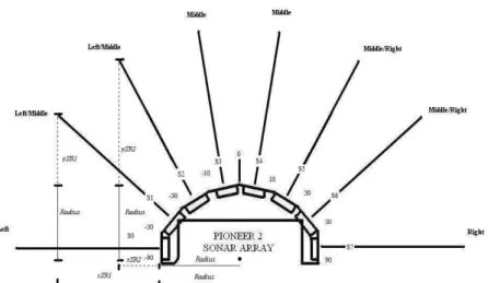
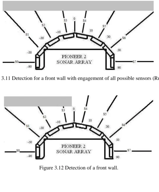
Figure 3.11 Detection for a front wall with engagement of all possible sensors (Rule 6). 34 Figure 3.12 Detection of a front wall. 34

Figure 3.13 A left-hand corner detected by the mobile robot (Rule 7) 35

Figure 3.14 The mobile robot travelling in a corridor (Rule 9). 36

Figure 3.15 A dead-end detected by the mobile robot (Rule 10) 36

Figure 4.1 Cluttered objects classified as a front wall by the mobile robot 39

Figure 4.2 Approaching wall- like dis-neighbouring objects 39

Figure 4.3 Approaching corner-like cluttered objects 40

Figure 4.4 Approaching a plane with sonar sensor 4 failed 41

Figure 4.5 Approaching a cluttered environment with the failure of Sonar Sensor 2 42

Figure 4.6 Sonar Sensors 1 and 3 being assumed to be in working order 43

Figure 5.1 The systemic design of proposed scheme 46

Figure 5.2 Global coordinate system 47

Figure 5.3 The mobile robot in an open area 48

Figure 5.4 Detection of an object by a single sonar sensor. 49

Figure 5.5 Detection of an object by two neighbouring sonar sensors. 49

(7)

Figure 5.7 Object detected in the situation of two dis-neighbouring sonar sensors failed. 51

Figure 5.8 The four crucial sonar sensors. 52

Figure 5.9 The front wall detected by six sonar sensors. 54

Figure 5.10 A front wall detected by sonar sensors 54

Figure 5.11 A front wall detected by S2, S3 and S4. 55

Figure 5.14A front wall detected by S4, S5 and S6. 56

Figure 5.15 Front wall detected by S2, S4 and S6. 57

Figure 5.16 A front wall detected with S3 failure 58

Figure 5.17 A front wall detected with S4 failure. 58

Figure 5.18 A front wall detected in a cluttered environment with S3 fail. 59

Figure 5.19 A left wall detected by S0, S1 and S2. 60

Figure 5.20 A right wall detected by S7, S6 and S5 61

Figure 5.21 A side wall detected by S0 and S2 62

Figure 5.22 The side wall detects by S5 and S7. 63

Figure 5.23 A left wall is detected when S1 is failure 64

Figure 5.24 A right wall is detected when S6 is failure. 64

Figure 5.25 A left wall with S1 failed in a cluttered environment. 65

Figure 5.26 A corridor detected 66

Figure 5.27 A corridor is detected with S1 failure 67

Figure 5.28 A corridor is detected with S2 failure. 67

Figure 5.31 A cluttered type corridor is detected with S1 in the open range. 69

Figure 5.32 A cluttered type corridor is detected with S6 in open range. 69

Figure 5.33 A cluttered type corridor is detected with S1 and S6 in the open range. 70

Figure 5.34 A cluttered type corridor is detected with S1 and S6 failures. 70

Figure 5.35 Distinguishing a side wall and a corner 71

Figure 5.36 Detection of a left-hand corner. 72

(8)

Figure 5.38 Detection of a left-hand cluttered corner by S2, S3 and S5. 73

Figure 5.39 Detection of a right-hand cluttered corner. 73

Figure 5.40 Detection of a dead-end. 75

Figure 6.1 The quadrant system with the robot as origin (the black dot). 79

Figure 6.2 The mobile robot avoiding an obstacle. 83

Figure 6.3 The mobile robot avoiding a front wall. 84

Figure 6.4 The mobile robot’s heading system 84

Figure 6.5, The mobile robot gets out of a left hand corner. 86

Figure 6.6 The robot gets out of a dead-end and a corridor. 87

Figure 6.7 The mobile robot meeting two obstacles. 88

Figure 6.8 The mobile robot meeting two obstacles with front obstruction 89

Figure 6.9 The Chronis’ approach detecting the obstruction as several objects located front 90 Figure 6.10 The mobile robot meeting a cluttered obstruction 90

Figure 6.11 The mobile robot meets a side obstruction. 91

Figure 6.12 The mobile robot meeting a cluttered side obstruction 91

Figure 6.13 The mobile robot meeting a front inclined plane. 92 Figure 6.14 The mobile robot avoiding an inclined front wall. 93

Figure 6.15 The mobile robot meeting a left inclined plane. 94 Figure 6.16 The mobile robot meeting a right inclined plane. 94

Figure 6.17 The mobile robot meeting a special left end corner. 95

Figure 6.18 The mobile robot meeting a special right end corner. 96

Figure 6.19 The mobile robot meets the object in the corridor. 97

Figure 7.1 Environment 1 99

Figure 7.2 The trajectories of Environment 1 G1. 101

Figure 7.3 The trajectories for reaching G2 in Environment 1. 106

Figure 7.4 The specular return leading to a wrong decision 107

Figure 7.5 The trajectories for reaching G3 in Environment 1 110

Figure 7.6 The trajectories for reaching G4 in Environment 1 114

Figure 7.7 Environment 2. 118

(9)

Figure 7.9 Step 1 of Chronis’ approach. 121

Figure 7.16 Trajectories for reaching G2 in Environment 2 127

Figure 7.19 Experiment in Environment 3. 136

Figure 7.21Trajectories for reaching G2 in Environment 3 140

(10)

LIST OF TABLES

Table 1.1, Shows the linguistic description for figure 1.1. 5

Table 3.1 Saphira build-in error model. 22

Table 3.2 An example of a .p file. 25

Table 6.1 The method determining goal quadrant. 80

Table 6.2 Example of setting up the goal point in Colbert 81

Table 7.1 The results of environment 1 G1. 104

Table 7.2 The performance of structures detection for Environment 1 G1. 104

Table 7.3 The performance of structure detected with sensor failure for environment 1 G1 .105

Table 7.4 The results of reaching G2 in Environment 1. 108

Table 7.5 The performance of structures detection for Environment 1 in reaching G2. 109 Table 7.6 The performance of structure detected with sensor failure for environment 1 G2 .109

Table 7.7 The results of reaching G3 in Environment. 112

Table 7.8 The performance of structures detection in reaching G3 in Environment 1 113

Table 7.9 The performance of structure detected with sensors failure reaching G3 in Environment 1 113

Table 7.10 The results of reaching G4 in Environment 1 116

Table 7.11 The performance of structures detection for reaching G4 in Environment 1.116 Table 7.12 The performance of structure detected with sensors failure in reaching G4 in Environment 1 116

Table 7.13 Overall performance and success rate. 117

Table 7.14 Average structure detection performance 117

Table 7.15 Results of reaching G1 in Environment 2. 125

Table 7.18 Results of reaching G2 in Environment 2 128

Table 7.19 Performance of structures detection in reaching G2 in Environment 2 128

Table 7.20 Performance of structure detected with sensors failure in reaching G2 in Environment 2 129

Table 7.23 Performance of structure detected with sensors failure in reaching G3in Environment 2 132

Table 7.27 Overall performance and success rate 135

Table 7.28 Performance of average structure detection 135

Table 7.30 Performance of structures detection in reaching G1 in Environment 3 139 Table 7.31 Performance of structure detected with sensors failure in reaching G1 in

(11)

Environment 3 139

Table 7.36 Performance of structures detection for reaching G2 in Environment 3 144

Table 7.37 Performance of structure detected with sensor failure for reaching G2 in Environment 3 144

Table 7.39 Performance of structures detection for reaching G4 in Environment 3 146

Table 7.40 Performance of structure detected with sensor failure for reaching G4 in Environment 3 147

Table 7.41 Overall Performances and Success Rate for Environment 3 147

Table 7.42 Performance of Average Structure Detection 148

Table 7.43 Overall Performance and Success Rates 148

(12)

ABSTRACT

A strategy typically employed for mobile robot navigation in an unknown environment is to follow a nominal straight-line path to the goal point. During travelling on the nominal path, the robot uses distance information, e.g. derived from sonar sensors, and geometric information to determine the spatial relations between the robot and the environment. Navigation in an unknown environment is still a challenging issue especially in the presence of cluttered objects or obstructions.

There are two possible ways to path planning in an unknown environment: the first is to map the environment and navigate based on the map; the second is to assign a nominal path, which the robot follows whilst at the same time it senses obstacles and reacts to achieve a collision free trajectory. In both cases the robot circumnavigates obstructions and generates a new path from the initial location to the goal point. Often the strategies used for navigation employ simple path planning techniques aided by specific methods to recognize objects and construct a structure for the environment. In Chronis’ PhD thesis is this area, a ring of low level sonar sensors is used to get spatial relations between a mobile robot and its environment. The eventual goal is to use spatial relations for navigation of the mobile robot in an unstructured, unknown environment. However, Chronis’ work does not construct any model of perceived structures in the environment and does not involve any tolerance to sensor failure. The approach described in this thesis improves this earlier work in precisely these two areas.

The proposed approach uses low level sensors, such as sonar sensors, to achieve navigation in an unknown and cluttered environment. It integrates sonar sensors and geometric information to construct structures of the environment and consequently establish a system that navigates effectively and quickly through cluttered objects and obstructions. It is shown that this strategy achieves efficiency and effectiveness in mobile robot navigation. The approach is also shown to be robust and tolerant to sensor failures. The strategy is not dependent on the number or type of sensors on the robot and does not assume a particular type of robot; it can work with any sensory method that can provide an object representation in two dimensions.

(13)

Chapter 1 Mobile Robot Navigation in an Unknown Environment

1.1 Background and Motivation

The issue of navigation raises three questions: ―where am I?‖, ―where am I going?‖, and ―how should I get there?‖ It essentially consists of two problems, (a) the problem of localisation arises from the question ―where am I?‖ and deals with the issue of determining the position in a particular environment [Kayton (1989), Rau (2003)], and (b) on the other hand, the problems of path planning and path following arise from the questions of ―where am I going?‖, and ―how should I get there?‖ respectively (see Chapter 2 for more details in navigation). Consider the case of a mobile robot, moving from a Point (S) to another point (G). The robot has to plan a path from S to G by avoiding obstacles and possibly also satisfying other constraints such as optimizing the time taken, and utilizing minimal amount of energy. In order to achieve the above mentioned goals, the robot has to (a) plan a path and (b) travel along this path to the goal point. In other words, the path planning problem can be divided into global path planning and local path planning which is essentially obstacle avoidance. The problem of path planning can be categorized into a) path planning in a known environment and b) planning a path in an unknown environment.

In a known environment, global path planning requires the knowledge of the environment, and the planning algorithm generates a set of nominal points by which the robot will pass. A local navigation system executes the same steps as in the global path planning, by comparing the robot‘s current position with positions stored in the global model, planning local paths as needed and avoiding unexpected obstacles. The local navigation system therefore must be made aware of the continuous changes in the environment by the incoming data gathered from sensors. The purpose of local obstacle avoidance is to plan a safe path which will take the robot around unexpected obstruction. In the known environment, the information of the world is provided a priori, e.g. a) the geometric

(14)

features of the world are provided to the robot a priori; and b) the shape and location of obstacles are known to the robot. A collision free path can be found off-line, and followed online. The problem of path planning in a known environment has been actively and extensively researched [see e.g. Latombe (1991), Tan (2006), Duan (2004), Bruce & Veloso (2002), Weng (2005)].

However, it is the case that a robot will face a more general problem, where it has partial information or in the worst case no information of the entire environment. Since the robot has no pre-knowledge of the locations of the obstacles, it is not possible to plan a priori collision free path. There are two possible ways to path planning in an unknown environment: a) maps the environment and plan path based on the map, and b) assigns a nominal path, the robot follows the path and at the same time the robot senses and reacts for a collision free trajectory. The nominal path could be a straight path between start and goal points and the mobile robot will make online decisions to achieve the goal point and avoid collision along the way. A strategy often used on encountering an obstacle is to approach it, and then circumnavigate it by using the currently available information. Thus while navigating around the obstacle, the robot, at every instant, determines whether there is a path towards the goal. When such a path becomes feasible, the robot leaves obstacle and starts to move towards the goal once again. In such situations, the robot must gather information by using its sensors to explore the environment while moving and modifying its plans accordingly. Most navigation algorithms for an unknown environment do not attempt to optimise the length of the path because the safe circumnavigation is more concerned than the construction of a minimum length path. This is in contrast to the navigation in a known environment where path planning can be essentially reduced to one of finding optimal path in the given environment. However the path planning in an unknown environment also concerns with keeping computational overhead low, and achieving greater efficiency, robustness and fault tolerance ability.

The answer to the question of ―where am I?‖ is generally the robot determines coordinates of its current position. In an unknown environment this is often not the

(15)

completed answer. This is because this requires further information, for example the robot is in a corridor, corner or facing a front wall. The answers to the questions ―where am I going?‖, and ―how should I get there?‖ in an unknown environment are given by the desired goal point, and a nominal path respectively. Thus in an unknown environment, when the robot meets an obstacle, it could circumnavigate it and generate another nominal path from there to the goal point. This could lead to the associated problem of minimizing deviations from a nominal path.

There have been a number of studies in this area [Wang (2004), Saffiotti (2000), Ye (2000), Seraji (2002), Arkin (1998), Dudek (2000), C.Ye (2009), J.Ng (2010)]. Often the strategies employ simple path planning but have specific methods to recognize objects and develop a structure for the environment. Wijk and Christensen [Wijk (2000)] provided a solution for the cluttered environment, using data obtained from sonar sensors. However, their method is deterministic in the sense that they did not incorporate any uncertainty in the detection of edges of objects within the vicinity of the robots themselves and in addition it does not incorporate any element of tolerance to sensor failure [Wijk (2000), Kambhampati, (2003)]. Chronis‘ work [Chronis (2002, 2007)] provides a different perspective for path planning. It shows how linguistic expressions can be generated to describe the spatial relations between a mobile robot and its environment, using readings from a ring of sonar sensors. The eventual goal is to use low level sensors such as sonar, that generates linguistic description for navigation of the mobile robot in an unstructured, unknown, and possibly dynamic environment. It generates linguistic descriptions that represent the qualitative state of the robot with respect to its environment, in terms of which are easily understood by human users. Thus an exact model of the environment is not built, but an approximation of the local environment is generated. The robot used by Chronis is a Nomad 200 robot with 16 sonar sensors evenly distributed around the robot. The sensors‘ readings are used to build an approximate representation of the objects surrounding the robot. During detection sonar sensor returns a range value which is less than the maximum, indicating that an obstacle has been detected. On the other hand when sonar sensors return the maximum value, it

(16)

means that no obstacle has been detected. However the depth of the obstacle cannot be determined from the sonar reading. In the case of multiple sonar returns, a question arises as to whether adjacent sonar readings are from a single obstacle or multiple obstacles. Chronis‘ solution [Chronis (2002)] is to determine if the robot can fit between the points of two adjacent sonar returns. If the robot cannot fit between two returns, then they consider these returns to be from the same object. Even if there are actually two objects, they may be considered as one for the purposes of navigation. In the case when the distance between the two points of the sonar returns is big enough to allow the robot to travel through, the method considers this situation as separate objects. For example, this linguistic approach is illustrated by Figure 1.1 and Table 1.1. Object 1 is on the left of robot. The obstacles behind the robot are recognized as a single object (Object 2). The obstacle to the right of the robot is detected as three different objects. Since there are only three sonar readings from the right obstacle, and they are far apart according to the distance measure, the readings may not be from a single obstacle.

Figure 1.1a The sonar detection the robot in the situation of Part B; Figure 1.1b, The robot detects 5 objects.

(17)

Table 1.1 shows the linguistic description for Figure 1.1.

There are other methods similar to Chronis approach are developed [see Gribble et al (1998), Perzanowski et al (1999), Shibata (1996), Stopp (1994), Freeman (1975), Bloch (1999), Miyajima and Ralescu, (1994)].

1.2 Research Hypothesis, Thesis Aims and Objectives

Problem of path planning in an unknown environment is complex, computationally intensive and involves uncertainties of many kinds e.g. sensors, environments etc. Although the approach in this thesis is designed to use low level sensors, such as sonar sensor, to achieve the navigation in an unknown and cluttered environment; that integrates sonar sensors and geometric information to construct structures; that achieve more efficiency which consequently to establish a navigation system with quicker response, more effectiveness and more successful runs. As a result, the common uncertainties of sonar sensors are angular uncertainty and specular return, for the robustness of the approach that in order to tolerant these uncertainties and in addition the fault tolerance to sensor failures also becomes a feature for this approach.

“Object 1 is mostly to the left of the Robot but somewhat forward ”

“Object 2 is behind the Robot but extends to the left relative to the Robot ”

“Object 3 is mostly to the right of the Robot but somewhat to the rear”

“Object 4 is to right of the Robot”

“Object 5 is mostly to the right of the Robot but somewhat forward ”

(18)

The thesis will address following issues:

 In comparison with Chronis‘ approach which does not build any structures of environment and only gives the rough location of the detected object, can more sense be made about the environment based on homogenous sonar sensors?

 The approach must work with cluttered and irregular shaped objects while Chronis‘ approach is more like survivals in a structured environment.

 What happens in the event of a sonar sensor failure? Would the robot be capable of navigating safely to the goal point?

Thus the aim of this thesis is to develop path planning strategy for a mobile robot that would enable it to move from a starting point to goal point. It can gather information from environment based on a set of homogenous sonar sensors, in order to provide a structured view of the environment rather than rough locations. It should perform the task of reaching the goal point in a cluttered environment without collision, and even in event of sensor failure(s).

This research is aimed to achieve the following objectives:

 To develop and analyse an algorithm that can use sonar information and provide more information regarding the environment, in that it should classify environment into structures.

 To develop a path planning approach that can navigate the robot from a given starting point to a goal point, while using the structural information represent environment.

(19)

 To set up experiments to verify the algorithm this provides structural classification.

 To set up experiments to test path planning approach and to compare with existing approaches, e.g. the the approach of Chronis.

1.3 The Structure of the Thesis

The algorithm in this thesis is implemented, verified and tested on the Saphira simulation platform. In Chapter 2, the approaches to navigation and path planning are reviewed. As the robot moves around, it gathers information by using sonar sensor. The information is used to classify the environment into a structure view. In order to do this, an algorithm is developed which is described in Chapter 3. There are uncertainties associated with sonar sensors, e.g. sonar specular return which causes wrong reading and results a bad classification or a poor path planning. This then leads to the issue of robustness of the approach. The algorithm should be able to carry on working in the presence of poor sensor information and failure of sensors. Chapter 4 deals with this particular aspect. Results are presented, The test results and verifications of the classification rules will be shown in Chapter 5 and the local avoidance strategies for each structure are introduced in Chapter 6. Chapter 7 reports the experiments and results of this project. The conclusion and future work can be found in Chapter 8.

(20)

Chapter 2 The Fundamentals of Mobile Robot Navigation

2.1Introduction

Robots are growing in complexity and their use in industry is becoming more widespread. The main use of robots has so far been in the automation of mass production industries, where the same, well defined tasks must be performed repeatedly in exactly the same fashion. However this project deals with the issue of navigation for a mobile robot. The mobile robot can be used in many areas, for example, office delivery, providing tours to museum visitors, exploring an unknown environment [C.Ye (2009), J.Ng (2010)] and etc. A mobile robot should be able to move in an environment with little or no human interference and it should be able to sense and react to its environment intelligently [Alonzo (1996)]. Although the robots seen in the science fiction movies appear to navigate with precision, in reality mobile robot navigation is a difficult research problem. Indeed, to simply let robot to navigate itself in a truly autonomous fashion is a serious challenge for today‘s mobile robots. Robot navigation is defined as the guiding of a mobile robot to a desired destination or along a desired path in an environment characterized by terrain and a set of distinct objects, such as obstacles and landmarks [Cao (1999)].

In this chapter the basic issues of mobile robot navigation is discussed. The problem of navigation essentially consists of the following questions:

 ―Where am I?‖ which is essentially the localisation problem.

 ―Where am I going?‖ and ―How can I get there?‖ is the path planning problem including online decision path plan and obstacles avoidance.

The solution to localisation problem allows the robot to know where it is. Later on in this chapter the problem associated with localisation are discussed. The localisation of mobile

(21)

robot can be classified into two categories: (a) reference based localisation, also called absolute position measurements, e.g. landmark navigation, active beacons and etc; and (b) dead-reckoning, also called relative position measurements which include odometry, and inertial navigation.

The second issue of navigation is path planning. The approaches to path planning can be broadly classified into two categories: model based path planning, whereby complete information on the environment is available a priori and the task is to find a collision-free path, and non-model based path planning, whereby the robot has to rely on its sensors for obtaining information on the environment. These approaches will be briefly reviewed in section 2.4 of this chapter.

2.2The Issue of “Where I Am”.

The issue of ―where I am‖ is crucial for the robot because it allows the robot to localize itself; in other words position itself in the environment. This would then allow it to navigate the environment efficiently. Dead-reckoning is the process of determining current position by using course, speed, time and distance to be traveled, e.g. using odometry. The absolute positioning techniques, for example landmark navigation, use the landmarks‘ coordinates and shapes to determine robot‘s position. As the robot finds these landmarks, its position can be calculated. Due to the lack of a single good method, developers of mobile robots usually combine two methods, one from each group [Borenstein (1996)]. The two groups can be further divided into the following seven categories:

I: Relative Position Measurements (also called Dead-reckoning) 1. Odometry

2. Inertial Navigation

(22)

3. Magnetic Compasses 4. Active Beacons

5. Global Positioning Systems 6. Landmark Navigation 7. Model Matching

Odometry is the most widely used navigation method for positioning a mobile robot, which has advantages of short-term accuracy, cost-efficiency and high sampling rates. However, it also has an innate disadvantage, an accumulation of a variety of errors, which might result from the integration of incremental motion information over time. For example one type of error, orientation error will cause large positioning errors, which can increase proportionally according to the distance covered by the robot (Borenstein 1996). Borenstein and his colleagues (1996) categorized errors into two kinds: systematic and non-systematic errors. Systematic errors are those originating from kinematic imperfections of the robot, for example, unequal wheel diameters or uncertainty about the exact wheelbase. Non-systematic errors are coming from the interaction of the floor with the wheels, for example, wheel slippage or bumps and cracks. As a result, Borenstein (1996) and his colleagues developed a method, UMBmark for quantitatively measuring systematic odometry errors, to measure non-systematic errors to some extent. Borenstein and Feng (1995) also proposed a method for measuring non-systematic errors, called Extended UMBmark, which can be used for comparison of different robots under similar conditions. Although as far as the measurement of non-systematic errors is concerned, there are restrictions since it is heavily dependent on the floor characteristics, although its merit cannot be denied. Owing to a system of well-defined floor irregularities, in response to non-systematic errors, the UMBmark procedure can give susceptibility to a different-drive platform. See more details from Borenstein and Feng (1994, 1995, and 1996). In this project the Sappire Simulation System includes errors concerning realistic simulation

(23)

2.3The Issue of “Where I Am Going” and “How I Can Get There”.

The questions of ―where I am going?‖ and ―how I can get there?‖ are generally the genesis of a plan, i.e. a path to a specified goal and the ability to execute this plan and to modify the plan as necessary to avoid unexpected obstacles [Crowley (1985)], being called path planning. It is important to ensure that the robot avoids collision. The path planning problem can be divided into global path planning and local obstacle avoidance (obstacle avoidance unit). Global path planning requires the pre-knowledge of the environment, and the planning algorithm generates a set of nominal points which schedules the robot actions. A local navigation system executes the steps in the global plan, compares the robot‘s current position with the positions stored in the global model and plans local paths as needed to avoid unexpected obstacles. The local navigation system therefore must be made aware of the continuous changes in the environment by the incoming data from different sensors located at strategic positions onboard. Sensor fusion requires a good knowledge of each detector‘s response function to provide accurate resolution of systematic errors that result from inappropriate interpretation of the sensor data. The purpose of local obstacle avoidance is to plan a safe path which will take the robot around unexpected obstacles.

The navigational task of a robot cart moving on a flat floor of an obstacle-filled room is the subject of the work by Cahn [Cahn (1975)]. Starting from an initial vehicle location, the robot is to move to an externally specified new location or goal as directly as possible without colliding with any stationary or moving obstacles. The obstacles on the nominal path can be detected by sensors. The robot generates the obstacles avoidance path, and modifies the speed, turning angle etc. Within the spatial constraints imposed by the obstacles, this approach assumes the spatial constraints to be a simple structure such as a wall, a corner and etc; the trajectory must be formed and the robot moves along it until the robot comes back to the original nominal path. In general robot path planning in a known environment can be defined as:

(24)

Given a description of the environment, the robot plans a path from starting point to the goal point without collision. The solution path between the starting point and goal point must collision free and allow some clearance space between the obstacles and the robot. The solution path should be the shortest or least computation one among possible paths between starting point and goal point.

Path planning in an unknown environment has to be performed based on the information obtained from the sensors, which usually consists of the radial range and the azimuth. The radial range which is the distances of the obstacles from the robot and the azimuth which is the angle between the radial range and one the fixed axes of the robot‘s reference system. In the known environment, the main concern for path planning is to find an optimal path in the given environment. Navigation algorithm for an unknown environment does attempt to optimise the length of the path because the safe circumnavigation is more of an overriding concern than the construction of a minimum length path at the same time concern of computational overhead, related articles [C.Ye (2009), J.Ng (2010) ].

2.4Navigating the Environment

Navigation has become a subject of significant interests in the modern world because it is open to a broad range of possible applications. Solutions of path planning algorithm have been proposed since the 1970s. A path planning algorithm among polyhedral obstacles based on the geometry graph was proposed in 1979 [Lozano-Perez (1979)]. Lumelsky and Stepanov [Lumelsky and Stepanov (1987)] considered the case where the automaton is a point and the environment is a subset of the two dimensional plane. The environment is assumed to be filled with unknown obstacles of an arbitrary shape and size. The information about the obstacles comes from a simple sensor whose capability is limited to detect an obstacle only when the robot hits it. In other words the information about the environment has a local character, i.e., information only about the immediate surrounding is available. Since the information about the environment is incomplete, the plan cannot

(25)

be pre-planned, and so its global optimality is ruled out. The advantage of using a point robot in two dimensions is the reduction of options available to it when encountering an obstacle, since it can turn left or right along the obstacle boundary. The only available input information includes the robot‗s own co-ordinates and those of the target. The environment is a plane with a set of obstacles, finite in number, that do not touch one another, and the points start S and target T in it. The motion capabilities of the mobile robot include the following: (i) move from starting point to target point on a straight line, (ii) move along the obstacle boundary, and (iii) stop. A local direction is either left or right once an obstacle has been hit. The algorithm defines a hit point H on an obstacle, while moving along a straight line towards the target, and the robot contacts the obstacle at the point H. It defines a leave point L on an obstacle, while it leaves the obstacle at the point L in order to continue its straight line path toward T. All hit and leave points are recorded during the exploration of the environment from S to T. Two algorithms are proposed, BUG1 and BUG2, the former being rather conservative and latter more humanlike.

Iyengar etal [Iyengar (1987)] incorporated learning by moving the robot through an unknown environment and incrementally constructing a visibility graph of the environment. Learning takes place as the robot visits a number of destination points. The point robot can memorise the vertices of the obstacles it visits. This technique assumes that the unexplored terrain is filled with disjoint convex polygonal obstacles which are mutually nonintersecting and no touching. In this approach, the visibility graph VG is constructed as follows: (i) V is the set of vertices of the obstacles; (ii) E is the set of edges of the graph. A line connecting the vertices V_iand V_j forms an edge



V_i,V_j



E.

Initially, VG is completely unknown. During the navigation process the robot constructs the learned visibility graph (LVG) consisting of the vertices and edges that have been traversed. Eventually the LVG should converge to VG. Suppose that the robot has to move from a straight point S to a target point T. Initially the robot moves along the straight line ST designed by the unit vector nst



(26)

Subsequently, it circumnavigates the obstacle using a local navigation strategy. Upon meeting the obstacle two directions are possible in going round it, 1



n and 2 

n . The local

optimisation criterion is defined as follows: max (nst 

. 

n), where 

n is unit vector along the direction of motion. Meanwhile, the procedure also incorporates a learning phase to acquire VG. This method was extended by Kant and Zucker [Kant (1988)] and Kyriakopoulos and Saridis [Kyriakopoulos and Saridis (1993)].

An approach based on vector field histogram was developed by Borenstein and Koren [Borenstein and Koren (1991)]. This approach generates both a direction and speed for the robot. However the disadvantage is that this approach ignores velocity and acceleration constraints on robot‘s motion.

Recently behaviour based approach has been developed. Yen and Pfluger [Yen and Pfluger (1995)] reflects the increasing interest in the potential of fuzzy logic in mobile robot navigation. The mobile robot considered by the authors in their work has a behavioural repertoire of actions, each suitable for a particular situation and is essentially a reactive control approach to selection of behaviours. There are two directions of movement to choose from, the desired direction and the allowable direction. The decision making process is to take the fuzzy variable that results as the minimum at any point between the desired direction and allowable direction, and then take the maximum point in that variable. The defuzzification process may produce a direction of movement that is close to the desired one, when it could have avoided collision by not altering its direction at all and thus save energy. Situation like this arises because fuzzy controls are used without the need to optimise some measure of performance and the lack of a detailed mathematical model may result in manoeuvres beyond the capabilities of the mobile robot.

Research in this area by Michon and Denis [Michon (2001)] provides insights into how landmarks are used for human navigation and what are considered to be key route points.

(27)

Another alternative strategy is that developed by Kuipers which combined qualitative and quantitative space representations into the spatial semantic hierarchy (SSH), to build a representation model of large-scale space. [Kuipers2000] The SSH models the human cognitive map and serves as a method for robot exploration and map building.

Kuipers and Byun [Kuipers (1991)] implemented the control, topological and metrical levels on a simulated robot with 16 range-sensors similar to the sensory system of the robot used in this work. In their experiments, the robot explores a simulated office environment and identifies a set of locally distinctive topological map elements (20 places and 23 edges), which are uses to construct a complete topological map.

Dai and Lawton used landmarks for qualitative robot navigation. [Dai (1993)] However, the algorithms completely ignore range estimates of landmarks. Determining robot position, when landmarks are indistinct, depends on recognizing the distribution of landmarks surrounding a robot.

Levitt and Lawton took a similar approach with the intention to prevent the error in robot navigation from accumulating, as it is common in techniques such as triangulation, ranging sensors, stereo techniques, dead reckoning, inertial navigation, correspondence of map data with the robot‘s locations and local obstacle avoidance techniques. [Levitt (1990)] Inspired by human and animal navigation performances which use extremely poor range estimates and very coarse angular information, Levitt and Lawton used distinctive landmarks to navigate a robot. A major constraint in spatial representation is the uncertainty in the absolute position of almost everything in the world, including robot position and the position of landmarks.

Nourbakhsh et al. used color vision and odometric information for robot navigation [Nourbakhsh (1999)]. To alleviate the poor information content of range-finding sensors, they made use of artificial colored landmarks that the robot is able to recognize. This is another landmark-based technique that works well if modifications to the environment are

(28)

allowed. Suitable environments would be museums (such as the one used for the robot, Sage of the Carnegie Museum of Natural History, which was one of the applications of Nourbakhsh‘s technique), office buildings, etc. [Nourbakhsh (1999)].

A solution to the problem of creating an accurate global topological map comes from Simhon and Dudek. They chose to use quantitative environment information to create local metric maps, which they used to form a global map [Simhon (1998)]. Assuming that a method to generate the local map already exists, the problem becomes one of choosing an area suitable to create a local map which is accurate and effective. Hence, they derived a measure of distinctiveness between different regions in the environment.

A qualitative approach to robot navigation using schematic maps is that of Freksa et. al. [Freksa (2000)]. Freksa et. al. formulate a model that uses qualitative spatial relations for robot navigation based on schematic map. A schematic map is a reduced detail topographical map as opposed to a sketch map, which is generated from abstract mental concepts and verbal descriptions.

In [Muller (2000)] an approach is proposed that enables a wheelchair to follow a route in a building, based on landmark recognition. Muller et. al. assume that the robot operates strictly in a building environment, so the problem of landmark recognition becomes one of corridor detection and orientation. The landmarks used in the [Muller (2000)] approach are: wall in front, corridor left, corridor right, door left and door right. The route is composed of a series of statements, each of which defines a navigation command (turn right, follow corridor, enter left door, etc.) upon sensing a particular arrangement of landmarks (corridor right, right hand bend, etc.). The algorithms of this work attempt to generalize the definition of landmarks to be any object or combination of objects and not strictly corridors, walls or entrances. Sonar sensors are also used as the sole source of sensory input. The algorithm is further developed by Chronis. Chronis‘ work [Chronis (2002, 2007)] provides a different perspective for path planning. As mentioned in Chapter 1, the navigation issues always high computational calculation and involve with high

(29)

level sensors such as vision, etc. Chronis uses low level sensors to generate linguistic descriptions of spatial relations between robot and environment. His eventual goal is to use these linguistic descriptions for navigation of the mobile robot in an unstructured, unknown, and possibly dynamic environment. Thus an exact model of the environment is not built, but an approximation of the local environment is generated.

2.5 The Proposed Path Planning in This Thesis

The approach, proposed in this thesis, which can be applied in a cluttered, unknown environment, provides the mobile robot with an egocentric structured environment, such as left wall, front wall and right end corner etc. In Chapter 3, a method is developed to obtain a representation of the structure, and its classification with the help of rules. The robot should recognize its structure in terms of egocentric spatial relations between itself and obstruction in its environment. It is also proposed with fault tolerance ability, i.e. determination of classification of structures can be carried out when sonar sensor fails. To achieve these, 3 types of status for the sonar sensors are defined: a) sonar sensor is said to be engaged when the reading is less than the maximum (object/obstacle detected), b) Sonar sensor is in operational status but has maximum distance return, this situation means the sonar sensor detects no obstructions, c) Sonar sensor fails, in the situation sonar sensor have no return value. The details of detection and classification algorithms will be introduced in Chapter 3.

However, uncertainty in the detection can be overcome by using the notion of consensus of sensors while at the same time increasing the tolerance to sensor failures. The other objective of the algorithm is to provide a fault-tolerant operation of the robot. This thesis presents a navigation method which overcomes uncertainty in the detection of objects and surfaces by using consensus sensors, while at the same time increasing the tolerance to sensor failures. This technique can be used for navigation in both known and unknown environments. It is developed to ensure that the robot moves from its current location to some desired locations. It should be noted that the primary aim is to perform the task but

(30)

not to increase the computational overhead.

For mobile robot to successfully plan its path in unstructured or unknown environments it not only needs to gather the right quality and quantity of information, also needs to make sense of this information, and make use of this information efficiently in order to be able to modify its path. Our approach fuses the information from eight sonar sensors in a consensus method and thus provides geometric information to make sense of the environment. The advantages of homogeneous sensors fusion are reducing fusion complexities, and allowing fusion at the sensor data level. Furthermore, the multi configuration sensors can be applied in the construction of geometric based world representations. [Bajcsy & Allen (1985), Chen & Medioni (1991), Porrill (1988)]

The path planning scheme developed in this thesis can be applied in an unknown environment. The nominal path is a straight line from the starting point which is the mobile robot‘s initial position to the desired position. Our approach has enhanced detection ability when the mobile robot meets a clutter of obstacles in an unknown environment; it gathers the geometric information of the surrounding obstacles and classifies these obstacles into structures such as wall, corner and etc. The eight sonar sensors can be thought as a network of consensus sensors which make a decision and at the same time they can be thought as eight individual sonar sensors which are mounted on the robot. During the observation, the decision will be made by at least three votes from 3 different sensors. The approach allows a cluttered unknown environment to be transformed into basic structured environment in mobile robot‘s view. For example, in the situation of Figure 2.1, when the mobile robot meets the obstacles, its decision making process, using information from sonar sensors, will view obstructions as a whole blocking like a front wall. The mobile robot classifies those obstacles as walls (virtual walls). The avoidance strategy will lead the robot to avoid the clutter of obstacles as avoiding a wall. Once the mobile robot reaches a clear area, the mobile robot will head to the goal point again. However the obstructions are not a front wall, so it can be thought as a virtual wall. When in the same situation, Chronis‘ approach detects the situation in stage 1 Figure 2.1

(31)

as three objects.

(32)

Chapter 3 Rules for Classification into Structures by Using Multiple

Homogenous Sonar Sensors

3.1 Introduction

In this Chapter, Saphira environment and Pioneer simulator are introduced. The Pioneer simulator has eight homogenous sonar sensors which can be thought as distributed and networked sensors. The essential geometric and distance information for designing the classification rules can be gathered by fusing homogenous sonar sensors. The details can be found in later sections in this chapter. The rules classify the environment into a simpler world which can be rebuilt with 16 primitive structures: an open area, an object, a virtual object, a front wall, a virtual front wall, a left wall, a virtual left wall, a right wall, a virtual right wall, a corridor, a virtual corridor, a left corner, a virtual left corner, a right corner, a virtual right corner and a dead-end.

To navigate in the environment, a mobile robot must sense the environment in order to know where it is. An autonomous mobile robot has to be able to sense the environment, and make decisions with no human interference. In order to make a correct decision, it is important that the robot senses its environment accurately, e.g. by using sonar and vision sensors. Using sonar sensor, it can map the seafloor [Morgan (1998)]. Even for an object in space, its position, size, shape, velocity and direction of motion can be determined. Kuc and Siegel have shown sonar scans also can use in everyday indoor environments [Kuc and Siegel (1987)]. In this thesis, the mobile robot uses sonar sensors for detecting obstructions.

Mobile robot uses fused information to construct a structure view of the environment. The fusion combines individual distance and geometric information, which are aggregated under certain rules by each sonar sensor. Most of the research in the area of multi-sensor robotics focuses on the application of multiple homogeneous sensors. The

(33)

homogeneous sensors fusion is computationally efficient in that the fusion complexities are reduced, and it allows fusion at the sensor data level (low level, a common information representation). Furthermore, the multi-configuration sensors were suggested in the construction of geometry-based world representations, which include multiple ultrasound sensors and multiple vision sensors. Single-sensor systems are inherently limited in their ability to provide a consistently reliable stream of information due to view-point occlusions, innate uncertainty, limited operating range and accuracy, individual sensor biases, spurious errors, and other factors attributable to employing only one sensory modality. In contrast, a properly employed synergistic multi-sensor configuration possesses the potential to provide:

(i) information from multiple viewpoints. (ii) robust and fault-tolerant operation. (iii) extended spatial and temporal coverage. (iv) diverse properties of the environment. (v) improved accuracy.

(vi) less ambiguity.

In this thesis, Sahpira system is used for development and verification. Saphira is a robotics application developed at the Pioneer mobile robot platform. The Pioneer robot has eight sonar sensors and we can consider these eight sensors as distributed and networked sensors. The algorithm for fusing information requires voting from each sensor and then reaching an agreement. In this thesis, the rules are designed for developing the geometric and distance information of these eight sensors. The problem of distributed consensus has historically existed in many diverse areas: Communication Networks [Mehyar, Spanos, Pongsajapan, Low and Murray (2005)], [Liu and Yang (2003)], Control Theory [Jadbabaie, Lin, and Morse (2003)], and Parallel Computation [Tsitsiklis (1984)], [Bertsekas, and Tsitsiklis (1989)].

(34)

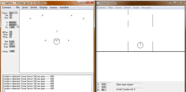
3.2 Saphira Environment and the Pioneer Simulator

Saphira has a C-like language, known as Colbert, for writing robot control programs. With Colbert, users can quickly write and debug complex control procedures, which are called Activities. Activities have a finite-state semantics that makes them particularly suited to representing procedural knowledge of sequences of actions. Activities can start and stop directing robot actions and other activities. Activities are coordinated by the Colbert executive, which supports concurrent processing of activities. Colbert comes with a runtime evaluation environment in which users can interactively view their programs, edit and rerun them.

Saphira comes with a software simulator of the physical robot and its environment, which allows users to debug applications conveniently. The simulator has realistic error models for the sonar sensors and wheel encoders (Table 3.1). The reality is such that, if a client program works with the simulator, it will work on the physical robot as well. The disadvantage of the simulator is that the environment model is an abstraction of the real world, with simple 2-D linear segments in place of the complex geometrical objects that real robot will encounter in the real world.

Parameter Pioneer Value Description

EncodeJitter 0.01 Error in distance

AngleJitter 0.02 Error in angular position

Table 3.1 Saphire build-in error model.

3.2.1 Representation of Space

Mobile robots operate in a geometric space, and the representation of that space is critical to robot‘s performance. There are two main geometrical representations: Local representation and Global representation. The Local Space is an egocentric coordinate

(35)

system a few meters in radius centered on the robot. The Global Space representation provides a larger perspective where objects are represented as a part of the robot‘s environment. The local space gives the robot a sense of its immediate surroundings. The test environment can be constructed in 2-D models, which is known as world models in Saphira. A world description file is a plain text document typically stored with the file name suffix .wld, which describes the size and contents of a simulated world. World models are abstractions of the real world, with linear segments representing the vertical surfaces of corridors, hallways, and the objects in them. The simulation environment 2 used in this thesis is shown in Figure 3.1 (the corresponding .wld file in the appendix):

Figure 3.1 The simulation environment 2.

3.2.2 Sonar Sensors on the Robot

Pioneer robots are a family of mobile robots with either two-wheel or four-wheel-drive. They are all small, intelligent robots, whose hardware architecture was originally developed by Kurt Konolige, of SRI International. In this thesis the simulator uses the Pioneer 2 parameters. The diameter of the Pioneer 2 is 250 mm. The Pioneer 2 mobile

(36)

robot has 8 sonar sensors in the front, distributed at a total of 180 degrees; range data obtained from these 8 sonar sensors can provide basic geometric and distance information about the environment. One motivation for using sonar sensors for mobile robot navigation comes from the impressive ultrasonic sensing capabilities of bats, which rely on echolocation to determine their position and to hunt their prey [Armingol, 2004]. The essential condition for geometric navigation of a mobile robot is the ability to determine its position. The robot obtains the input data from the sonar sensors by movement in the map or virtual/real environment. The sonar sensor systems generally calculate distance by using the time of flight (TOF) method. Define d, as the distance between the sonar senor and object, c as the speed of sound and t as the time of sound wave traveling on both ways, the two way distance can be calculated by speed of sound multiply by the time traveling; the single way distance can be calculated refer Figure 3.2.

ct d 2 1  (3.1)

Figure 3.2 Sonar distance- measuring concept

In the simulation environment, a .p file, as shown in table 3.2, is used to store the basic parameters of the robot, and it must be loaded to form a simulated pioneer class robot. This file contains both geometric and kinematic details for the simulator such as radius of the robot and speeding parameter, etc. Figure 3.3 shows the Pioneer 2 robot in the simulation.

(37)

Table 3.2 An example of a .p file.

;; Parameters for the Pioneer 2 DX Mobile Robot

AngleConvFactor 0.001534 ; radians per angular unit (2PI/4096) DistConvFactor 0.826 ; mm returned by P2

VelConvFactor 1.0 ; mm/sec returned by P2 RobotRadius 250.0 ; radius in mm

RobotDiagonal 120.0 ; half-height to diagonal of octagon Holonomic 1 ; turns in own radius

MaxRVelocity 500.0 ; degrees per second MaxVelocity 2200.0 ; mm per second

RangeConvFactor 0.268 ; sonar range returned in mm ;; Robot class, subclass

Class Pioneer Subclass p2dx

SonarNum 8 ; 8 total sonars

;; These are for the eight front sonars: six front, two sides ;; Sonar parameters

;; SonarNum N is number of sonars

;; SonarUnit I X Y TH is unit I (0 to N-1) description

;; X, Y are position of sonar in mm, TH is bearing in degrees ;; # x y th ;;--- SonarUnit 0 115 130 90 SonarUnit 1 155 115 50 SonarUnit 2 190 80 30 SonarUnit 3 210 25 10 SonarUnit 4 210 -25 -10 SonarUnit 5 190 -80 -30 SonarUnit 6 155 -115 -50 SonarUnit 7 115 -130 -90 FrontBuffer 20 SideBuffer 40

(38)

Figure 3.3 The simulated pioneer 2 robot.

3.3 Geometric Information of Multi-sonar-sensor Configuration

A single sonar sensor only provides distance to the object without any other information, such as shape or orientation. In this thesis the robot considered has eight sonar sensors mounted on it and numbered from 0 to 7. Readings are defined as SR0, SR1 …SR7. From now on, these sensors will be labeled as Si, i=0…7. The robot can be thought of as a local coordinating system. The centre of the mobile robot will be the origin of the coordinating system. A sonar detected point can be transformed as a point with coordinates (xi, yi) in

the local system:

 cos * ) (SRi Radius x_i   (3.2)  sin * ) (SRi Radius y_i   (3.3) Note: Radius is the mobile robot‘s radius and  is the angle the sonar sensor mounted.

(39)

Figure 3.4 Illuminates the  value.

 has always a positive value, e.g  = 40 when the angle being considered is between S0 and S1; the robot is symmetrical, the angle between S6 and S7 is 40 degree. The angle between S0 and S2 is 60 degree, and the angle between S5 and S7 is 60 degree, hence  = 60. The angle between S0 and S3 and the angle between S7 and S4 are 80 degree, hence

 = 80, see Figure 3.4.

Xiand Yi are the notations for the distance from the detected point to the centre of robot;

and the absolute value of xi and yi. The distances from the detected point to the robot are

shown in the following formula:



xSRi |(SRiRadius)*cosRadius|

= |x_iRadius| (3.4) And



ySRi |(SRiRadius)*sinRadius|

(40)

Figure 3.5Classification of sensors and number of sensors (S0 to S7)

The sonar sensor can detect an obstaclefrom a distance of up to 2999 mm away. Consider that S1 detects an obstacle and returns a distance reading of 2999 mm. According to equations 3.4 and 3.5, xSR1 = 2240 mm and ySR1= 1840 mm, (see Figure 3.5). If the

returned reading is 2999mm then the value of S6 is the same as S1, so xSR6 = 2240 mm

and ySR6= 1840 mm. So the remaining sensor value as follow: xSR2 = 1375 mm and

ySR2= 2565 mm and xSR5 = 1375 mm and ySR5= 2565 mm; xSR3 = 315 mm and ySR3=

2950 mm and xSR4 = 315 mm and ySR4= 2950 mm. These distance information is

complementary for positioning how close the object is to the robot horizontally and vertically.

In case when the mobile robot is not too close to the obstruction, a safety parameter of distance, e.g. 200 mm, can be set, see Figure 3.6. Details of a safety module will be introduced in Chapter 6. Consider the case of each sonar sensor‘s reading when xSRi and

ySRi = 200 mm; the vaules of SRi can be calculated by substituting xSRi and ySRi = 200

mm into equation 3.4 and 3.5; For example, when xSR1and xSR6 = 200 mm, then SR1 and

SR6 = 338 mm, this distance information which provided by S1 or S6 detection range 338

mm is a boundary value, if SR1 or SR6 is less than 338 mm, there is a possible horizontally collision to the robot. Thus we calculate these boundary values for each sensor: when xSR2 and xSR5 = 200 mm, the boundary value of SR2 and SR5 = 650 mm;