Numerical Simulation of Frictional Contact Problems using Nagata Patches in Surface Smoothing

(1)

Diogo Mariano Simões Neto

NUMERICAL SIMULATION OF FRICTIONAL CONTACT PROBLEMS

USING NAGATA PATCHES IN SURFACE SMOOTHING

Doctoral Thesis in Mechanical Engineering, specialization in Production Technologies, supervised by Professor Marta Cristina Cardoso de Oliveira and Professor Luís Filipe Martins Menezes, submitted to the Department of Mechanical Engineering, Faculty of Sciences and Technology of the

University of Coimbra September 2014

(2)

Numerical Simulation of Frictional Contact Problems

using Nagata Patches in Surface Smoothing

A dissertation submitted to the Department of Mechanical Engineering of the University of Coimbra in partial fulfilment of the requirements for the

degree of Doctor of Philosophy in Mechanical Engineering

Diogo Mariano Simões Neto

September 2014

Scientific advisers:

Prof. Marta Cristina Cardoso de Oliveira,University of Coimbra, Portugal Prof. Luís Filipe Martins Menezes, University of Coimbra, Portugal

Dissertation defence committee:

President Prof. José Valdemar Bidarra Fernandes

Full Professor, University of Coimbra, Portugal Reviewer Prof. Pierre-Yves Manach

Full Professor, University of Southern Brittany, France Reviewer Prof. José Manuel de Almeida César de Sá

Full Professor, University of Porto, Portugal Reviewer Prof. Paulo António Firme Martins

Full Professor, University of Lisbon, Portugal Reviewer Prof. José Luís de Carvalho Martins Alves

Assistant Professor, University of Minho, Portugal Reviewer Prof. Amílcar Lopes Ramalho

Associate Professor, University of Coimbra, Portugal Member Prof. Marta Cristina Cardoso de Oliveira

(3)

(4)

To my family

“Everything must be made as simple as possible. But not simpler.”

(5)

(6)

Acknowledgements

iii

Acknowledgements

The research work present in this PhD thesis has been carried out in the last four years at the Department of Mechanical Engineering of the University of Coimbra. These four years of research were a very fruitful period in my engineering education, as well as in my personal development. The freedom in the investigation accompanied by a wise guidance of my scientific advisers allowed me to improve the knowledge in the field of computational contact mechanics.

I particularly wish to express my sincere gratitude to my scientific advisers Professor Marta Oliveira and Professor Luís Filipe Menezes, for the valuable guidance, support and consistent encouragement during my PhD thesis. I highly appreciate their outstanding scientific expertise and experience (shared with me), as well as the sincere friendship, trust and incessant care to provide me with the best possible working conditions. Their drive for scientific rigor have been indispensable to the successful and timely conclusion of this thesis and, at the same time, a great source of inspiration for me.

I would like to express my special thanks to Professor José Luís Alves for the fruitful discussions and critical remarks concerning the numerical implementation of the developed algorithms in DD3IMP finite element code, as well as for his friendship. His computational expertise, insightful comments and suggestions on the research direction were crucial for the success of this work.

I am grateful for the excellent support given within the Mechanical Engineering Centre of the University of Coimbra (CEMUC) chaired by Professor Valdemar Fernandes and the opportunity that was given to me to develop my research work, as well as the financial support to participate in some conferences. I also wish to thank all members of CEMUC for the friendly and scientifically inspiring atmosphere at the research centre. Additional thanks go to the Advanced Manufacturing Systems research group chaired by Professor Altino Loureiro, which has provided the computational resources necessary to run the numerical simulations.

(7)

iv

I would like to thank my colleagues of office and friends Álvaro Mendes, André Pereira, André Rodrigues, Henrique Santos, João Martins, Luis Reis, Pedro Barros, Pedro Prates, Rui Leal and Vasco Simões for their friendship and the many inspiring (scientific and several non-scientific) discussions we had. I wish to thank all my friends for their encouragement, in particular the laughs of Rafael Raposo and the deep knowledge in computer programming of the new sportsman Ricardo Heleno. I cannot forget to thank my big French friend Jérémy Coër for his unconditional friendship, help and some useful scientific discussions about sheet metal forming process.

Finally, I like to thank my family for the love and support they gave me, in particular to my parents and my brother for their encouragement, personal sacrifice and understanding through all the years. Without them it would not been possible to finish this work.

The financial support of this work has been provided by the Portuguese Foundation for Science and Technology (FCT) through the PhD Grant SFRH/BD/69140/2010, which is greatly acknowledged.

(8)

Resumo

v

Resumo

Todos os movimentos no mundo envolvem contato e atrito, desde andar até conduzir um carro. A mecânica do contacto tem aplicação em muitos problemas de engenharia, incluindo a ligação de elementos estruturais com parafusos, projeto de engrenagens e rolamentos, estampagem ou forjamento, contato entre os pneus e a estrada, colisão de estruturas, bem como o desenvolvimento de próteses em engenharia biomédica. Devido à natureza não-linear e não-suave da mecânica do contato (área de contato desconhecida a priori), tais problemas são atualmente resolvidos usando o método dos elementos finitos no domínio da mecânica do contato computacional. No entanto, a maioria dos programas comerciais de elementos finitos atualmente disponíveis não é totalmente capaz de resolver problemas de contato com atrito, exigindo métodos numéricos mais eficientes e robustos. Portanto, o principal objetivo deste estudo é o desenvolvimento de algoritmos e métodos numéricos para aplicar na simulação numérica de problemas de contato com atrito entre corpos envolvendo grandes deformações. Os desenvolvimentos apresentados são implementados no programa de elementos finitos DD3IMP.

A formulação quasi-estática de problemas de contato com atrito entre corpos deformáveis envolvendo grandes deformações é primeiramente apresentada no âmbito da mecânica dos meios contínuos, seguindo o método clássico usado em mecânica dos sólidos. A descrição cinemática dos corpos deformáveis é apresentada adotando uma formulação Lagrangeana reatualizada. O comportamento mecânico dos corpos é descrito por uma lei constitutiva elastoplástica em conjunto com uma lei de plasticidade associada, permitindo modelar uma grande variedade de problemas de contacto envolvidos em aplicações industriais. O contacto com atrito entre os corpos é definido por duas condições: o princípio da impenetrabilidade e a lei de atrito de Coulomb, ambas impostas na interface de contato. O método do Lagrangeano aumentado é aplicado na resolução do problema de minimização com restrições resultantes das condições de contato e atrito, produzindo uma formulação mista envolvendo deslocamentos e forças de contato.

(9)

vi

A discretização espacial dos corpos é realizada com elementos finitos sólidos isoparamétricos, enquanto a discretização da interface de contacto é realizado utilizando a técnica Node-to-Segment, impedindo os nós slave de penetrar na superfície master. A parte geométrica do elemento de contacto, definida por um nó slave e o segmento master mais próximo, é criada pelo algoritmo de deteção de contacto com base na seleção do ponto mais próximo na superfície master, obtido pela projeção normal do nó slave. No caso particular de contato entre um corpo deformável e um obstáculo rígido, a superfície rígida master pode ser descrita por parametrizações normalmente utilizadas em modelos CAD. No entanto, no caso geral de contato entre corpos deformáveis, a discretização espacial dos corpos com elementos finitos lineares origina uma representação da superfície master por facetas. Esta é a principal fonte de problemas na resolução de problemas de contato envolvendo grandes escorregamentos, uma vez que a distribuição dos vetor normais à superfície é descontínua. Assim, é proposto um método de suavização para descrever as superfícies de contacto

master baseado na interpolação Nagata, que conduziu ao desenvolvimento do elemento de contacto Node-to-Nagata. A precisão do método de suavização das superfícies é avaliada através de geometrias simples. Os vetores normais nodais necessários para a interpolação Nagata são avaliados a partir da geometria CAD no caso de superfícies rígidas, enquanto no caso de corpos deformáveis são aproximados utilizando a média ponderada dos vetores normais das facetas vizinhas. Tanto os vetores de segundo membro como as matrizes residuais tangentes dos elementos de contacto são obtidas de forma coerente com o método de suavização da superfície, enquanto o método de Newton generalizado é utilizado para resolver o sistema de equações não lineares.

O método de suavização das superfícies e os elementos de contacto desenvolvidos são validados através de exemplos com soluções analíticas ou semi-analíticas conhecidas. Também são estudados outros problemas de contato mais complexos, incluindo o contato de um corpo deformável com obstáculos rígidos e o contato entre corpos deformáveis, contemplando fenómenos de auto-contato. A suavização da superfície master melhora a robustez dos métodos computacionais e reduz fortemente as oscilações na força de contato, associadas à descrição facetada da superfície de contato. Os resultados são comparados com soluções numéricas de outros autores e com resultados experimentais, demonstrando a precisão e o desempenho dos algoritmos implementados para problemas fortemente não-lineares.

Palavras-chave:

Mecânica do Contacto, Método dos Elementos Finitos, Método do Lagrangeano Aumentado, Grandes Escorregamentos, Node-to-Segment, Suavização de Superfícies, Superfícies Nagata.

(10)

Abstract

vii

Abstract

All movements in the world involve contact and friction, from walking to car driving. The contact mechanics has application in many engineering problems, including the connection of structural members by bolts or screws, design of gears and bearings, sheet metal or bulk forming, rolling contact of car tyres, crash analysis of structures, as well as prosthetics in biomedical engineering. Due to the nonlinear and non-smooth nature of contact mechanics (contact area is not known a priori), such problems are currently solved using the finite element method within the field of computational contact mechanics. However, most of the commercial finite element software packages presently available are not entirely capable to solve frictional contact problems, demanding for efficient and robust methods. Therefore, the main objective of this study is the development of algorithms and numerical methods to apply in the numerical simulation of 3D frictional contact problems between bodies undergoing large deformations. The presented original developments are implemented in the in-house finite element code DD3IMP.

The formulation of quasi-static frictional contact problems between bodies undergoing large deformations is firstly presented in the framework of the continuum mechanics, following the classical scheme used in solid mechanics. The kinematic description of the deformable bodies is presented adopting an updated Lagrangian formulation. The mechanical behaviour of the bodies is described by an elastoplastic constitutive law in conjunction with an associated flow rule, allowing to model a wide variety of contact problems arising in industrial applications. The frictional contact between the bodies is established by means of two conditions: the principle of impenetrability and the Coulomb’s friction law, both imposed to the contact interface. The augmented Lagrangian method is applied for solving the constrained minimization incremental problem resulting from the frictional contact inequalities, yielding a mixed functional involving both displacements and contact forces.

The spatial discretization of the bodies is performed with isoparametric solid finite elements, while the discretization of the contact interface is carried out using the classical

(11)

viii

Node-to-Segment technique, preventing the slave nodes from penetrating on the master surface. The geometrical part of the contact elements, defined by a slave node and the closest master segment, is created by the contact search algorithm based on the selection of the closest point on the master surface, defined by the normal projection of the slave node. In the particular case of contact between a deformable body and a rigid obstacle, the master rigid surface can be described by smooth parameterizations typically used in CAD models. However, in the general case of contact between deformable bodies, the spatial discretization of both bodies with low order finite elements yields a piecewise bilinear representation of the master surface. This is the central source of problems in solving contact problems involving large sliding, since it leads to the discontinuity of the surface normal vector field. Thus, a surface smoothing procedure based on the Nagata patch interpolation is proposed to describe the master contact surfaces, which led to the development of the Node-to-Nagata contact element. The accuracy of the surface smoothing method using Nagata patches is evaluated by means of simple geometries. The nodal normal vectors required for the Nagata interpolation are evaluated from the CAD geometry in case of rigid master surfaces, while in case of deformable bodies they are approximated using the weighted average of the normal vectors of the neighbouring facets. The residual vectors and tangent matrices of the contact elements are derived coherently with the surface smoothing approach, while the generalized Newton method is used for solving the nonlinear system of equations.

The developed surface smoothing method and corresponding contact elements are validated through standard numerical examples with known analytical or semi-analytical solutions. More advanced frictional contact problems are studied, covering the contact of a deformable body with rigid obstacles and the contact between deformable bodies, including self-contact phenomena. The smoothing of the master surface improves the robustness of the computational methods and reduces strongly the non-physical oscillations in the contact force introduced by the traditional faceted description of the contact surface. The presented results are compared with numerical solutions obtained by other authors and experimental results, demonstrating the accuracy and performance of the implemented algorithms for highly nonlinear problems.

Keywords:

Contact Mechanics, Finite Element Method, Augmented Lagrangian Method, Large Sliding, Node-to-Segment Discretization, Surface Smoothing, Nagata Patches.

(12)

Résumé

ix

Résumé

Tous les mouvements dans le monde impliquent du contact et du frottement, depuis le simple fait de marcher à celui de conduire une voiture. La mécanique du contact trouve ses applications dans de nombreux problèmes d’ingénierie, comprenant par exemple la liaison d’éléments structurants par vis/écrou, la conception des engrenages et des roulements, l’emboutissage ou le forgeage, le contact entre les pneus et la route, l’analyse de la collision des structures, ou encore le développement de prothèses en ingénierie biomédicale. En raison de la nature non linéaire et non lisse du contact mécanique (la surface de contact exacte est a priori inconnue), de tels problèmes sont actuellement résolus en utilisant la méthode des éléments finis, dans le domaine du calcul scientifique de la mécanique du contact. Cependant, la majorité des programmes de calcul par éléments finis commerciaux, actuellement disponibles, n’est pas pleinement en mesure de résoudre les problèmes de contact avec frottement, qui exigent des méthodes numériques plus efficaces et plus robustes. Par conséquent, le principal objectif de cette étude est le développement d’algorithmes et de méthodes numériques, qui permettront de réaliser la simulation numérique de problèmes de contact avec frottement entre des corps impliquant de grandes déformations. Les développements présentés sont implémentés dans le code de calcul par éléments finis DD3IMP.

La formulation de problèmes de contact quasi-statique avec frottement entre corps déformables en grandes déformations est dans, un premier temps, présentée dans le cadre de la mécanique des milieux continus, en suivant le schéma classique utilisé en mécanique du solide. La description cinématique des corps déformables est présentée en adoptant une formulation Lagrangienne réactualisée. Le comportement mécanique des corps est décrit par une loi de comportement élasto-plastique, en conjonction avec une loi d’écoulement plastique associée, permettant de modéliser une grande variété des problèmes de contact survenants dans des applications industrielles. Le contact avec frottement établi entre les corps est défini par deux conditions : le principe de non-pénétration et la loi de frottement de Coulomb, toutes deux imposés à l’interface de contact. La méthode du Lagrangien augmenté est utilisée dans la résolution du problème de minimisation avec restriction

(13)

x

résultantes des conditions du contact et de friction, qui produisent une formulation mixte impliquant les déplacements et les forces de contact.

La discrétisation spatiale des corps est faite avec des éléments finis solides isoparamétriques, tandis que la discrétisation de l’interface de contact est réalisée en utilisant la technique du Node-to-Segment, empêchant ainsi aux nœuds esclaves de pénétrer la surface maître. La partie géométrique de l’élément de contact, définie par un nœud esclave et le segment principal le plus proche, est créée par l’algorithme de détection du contact sur la base de la sélection du point le plus proche de la surface maître, obtenue par la projection normale du nœud esclave. Dans le cas particulier du contact entre un corps déformable et un obstacle rigide, la surface rigide maître peut être décrite par des paramétrisations couramment utilisés dans les modèles de CAO. Toutefois, dans le cas général d’un contact entre corps déformables, la discrétisation spatiale des corps avec des éléments finis linéaires engendre une représentation bilinéaire de la surface maître par facettes. Il s’agit là de la principale source de difficultés dans la résolution des problèmes de contact impliquant de grands glissements, étant donné qu’elle conduit à une distribution discontinue du champ des vecteurs normaux à la surface. Ainsi, il est proposé une méthode de lissage pour décrire les surfaces de contact maître basée sur l’interpolation Nagata, qui a conduit à l’élaboration d’un élément de contact Node-to-Nagata. La précision de cette méthode de lissage des surfaces est évaluée au travers de géométries simples. Les vecteurs normaux nodaux nécessaires à l’interpolation Nagata sont évalués à partir de la géométrie CAO dans le cas de surfaces rigides, alors que dans le cas des corps déformables ils sont estimés à l’aide de la moyenne pondérée des normales des facettes voisines. Les vecteurs résiduels et les matrices tangentes des éléments de contact sont dérivés de manière cohérente avec la méthode de lissage de surface, tandis que la méthode de Newton généralisée est utilisée pour la résolution du système d’équations non linéaires.

La méthode de lissage des surfaces et les éléments de contact développés sont d’abord validés à travers des exemples numériques standards, dont les solutions analytiques ou semi-analytiques sont connues. D’autres problèmes de contact frottant plus évolués sont ensuite étudiés, en traitant le contact d’un corps déformable avec des obstacles rigides et le contact entre corps déformables, incluant les phénomènes d’auto-contact. Le lissage de la surface maître améliore la robustesse des méthodes de calcul et réduit fortement les oscillations non physiques de la force de contact, induite par la description traditionnelle facettisée de la surface de contact. Les résultats présentés sont comparés aux solutions numériques obtenues par d’autres auteurs ainsi qu’à des résultats expérimentaux, démontrant alors la précision et les performances des algorithmes mis en œuvre pour des problèmes fortement non linéaires.

Mots-Clés:

Mécanique du Contact, Méthode des éléments finis, Méthode du Lagrangien augmenté, Grand glissements, Discrétisation Node-to-Segment, Lissage de surfaces, Patch de Nagata.

(14)

Contents

xi

List of Figures

Figure 1.1. Sheet metal forming: (a) double-attached structural component (Courtesy of Rockford Toolcraft); (b) engine hood inner (Courtesy of Volkswagen

Autoeuropa). ... 3

Figure 1.2. Crash of a car against a deformable barrier (Courtesy of Daimler Chrysler AG): (a) frontal impact; (b) lateral impact. ... 4

Figure 1.3. Biomechanics applications for human joints: (a) knee implants [Morra 08]; (b) contact between lumbar vertebral bodies (Courtesy of Brigham Young University). ... 5

Figure 2.1. Reference and current configuration of a body B undergoing large deformations... 13

Figure 2.2. Schematic representation of the polar decomposition theorem... 14

Figure 2.3. Schematic representation of the multiplicative decomposition theorem. ... 17

Figure 2.4. Basic notation for the two body large deformation contact problem. ... 22

Figure 2.5. Parameterization of the potential contact surface for body 2. ... 23

Figure 2.6. Definition of the local coordinate system in the contact surfaces: (a) master surface; (b) slave surface. ... 25

Figure 2.7. Orthogonal projection of the slave point _xs_{onto the master surface. ... 26}

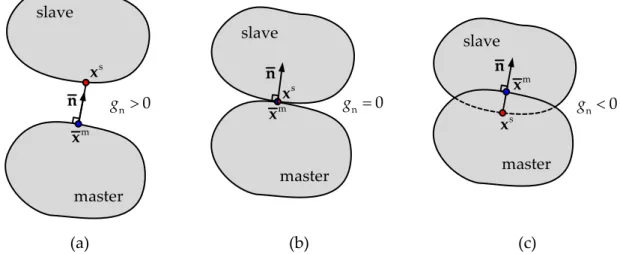
Figure 2.8. Three different geometrical conditions of the slave point with respect to the master body: (a) separated; (b) contact; (c) penetration. ... 26

Figure 2.9. Geometry related problems: (a) asymmetry of the closest point definition; (b) non-uniqueness of the closest point; (c) nonexistence of the orthogonal projection point. ... 28

(19)

xvi

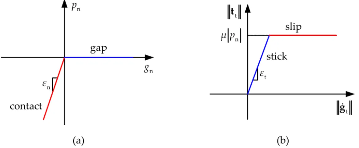
Figure 2.11. Unilateral contact law defined by the Karush–Kuhn–Tucker conditions. ... 33

Figure 2.12. Graphical representation of Coulomb’s frictional conditions: (a) relation between the norm of the tangential velocity and the norm of the frictional force vector; (b) relation between the contact pressure and the components of the frictional force vector (Coulomb’s frictional cone). ... 35

Figure 2.13. Physical interpretation of the penalty method: (a) initial configuration; (b) configuration after penetration; (c) equilibrium state [Yastrebov 13]. ... 39

Figure 2.14. Application of the penalty method to the frictional contact problem: (a) regularized unilateral contact law; (b) regularized Coulomb’s friction law. . 41

Figure 2.15. One degree of freedom contact problem example: (a) initial configuration; (b) deformed configuration due to the contact with a rigid wall. ... 50

Figure 2.16. Penalized energy functional for different values of penalty parameter and corresponding solution (hollow points). ... 51

Figure 2.17. Dependency of the penalty parameter on the spring system solution: (a) displacement; (b) contact force. ... 52

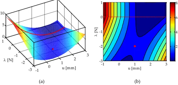
Figure 2.18. Lagrangian functional corresponding to the spring in contact with a rigid wall: (a) surface with a saddle point solution; (b) contour of the functional values and stationary point. ... 53

Figure 2.19. Augmented Lagrangian functional for the spring in contact with a rigid wall, using a unitary penalty parameter value: (a) surface with a saddle point solution; (b) contour of the functional values and stationary point. ... 55

Figure 2.20. Gradients of the augmented Lagrangian functional using unitary penalty parameter: (a) gradient with respect to displacement; (b) gradient with respect to Lagrange multiplier (force). ... 56

Figure 3.1. Global framework of finite element code DD3IMP. ... 61

Figure 3.2. Continuous body and its discretized representation using a finite element mesh composed by finite elements and nodes. ... 64

Figure 3.3. Isoparametric 8-node tri-linear hexahedral solid element. ... 66

Figure 3.4. Geometrical interpretation of the Newton–Raphson method. ... 67

Figure 3.5. Example of sparse matrix associated with the finite element discretization: (a) discretized unitary cube; (b) sparse matrix pattern (black dots represent nonzero entries). ... 71

(20)

List of Figures

xvii

Figure 3.7. Influence of the finite element mesh refinement on the: (a) elapsed time; (b) memory requirement. ... 76

Figure 3.8. Schematic illustration of different types of contact discretization: (a) Node-to-Node; (b) Node-to-Segment; (c) Segment-to-Segment. ... 77

Figure 3.9. Node-to-Segment contact discretization: (a) penetration conditions

unchecked in master nodes; (b) contact element composed by a slave node and a master segment... 79

Figure 3.10. Distribution of the vertical stress component for different choices of the master and slave surfaces in the NTS contact discretization: (a) finite element mesh of contacting cubes; (b) upper cube defined as master and lower as slave; (c) upper cube defined as slave and lower as master. ... 81

Figure 3.11. Distribution of the vertical stress component in the contact patch test using: (a) the single-pass NTS algorithm with the lower cube as master; (b) the two-pass NTS algorithm. ... 84

Figure 3.12. Distribution of the vertical stress component in the contact patch test adopting an unstructured mesh: (a) upper surface mesh; (b) lower surface mesh; (c) single-pass NTS discretization defining the lower cube as master; (d) two-pass NTS discretization. ... 85

Figure 3.13. Description of a rigid contact surface (half spherical shell) using: (a) finite element mesh; (b) parametric patches. ... 87

Figure 3.14. Vertical displacement distribution using linear finite elements to describe the cube: (a) 8-node tri-linear hexahedral; (b) 4-node linear tetrahedral. ... 88

Figure 3.15. Vertical displacement distribution using quadratic finite elements to describe the cube: (a) 20-node serendipity hexahedral; (b) 27-node tri-quadratic hexahedral. ... 89

Figure 3.16. Examples of failure of the global search algorithm based on the closest master node: (a) triangular master mesh; (b) quadrilateral master mesh. ... 93

Figure 3.17. Examples of grid of points created on the master surface: (a) triangular master mesh; (b) quadrilateral master mesh... 95

Figure 3.18. Example of self-contact in a thin walled structure: (a) difficulties in the contact with the reverse side; (b) proposed global search applied in 2 points. ... 97

Figure 3.19. Example of a slave node near a sharp corner/valley: (a) convex master

(21)

xviii

Figure 3.20. Definition of the slip increment vector for: (a) slave node in contact in the previous time step; (b) slave node not in contact in the previous time step. 103

Figure 3.21. Configuration of the problem composed by a flat surface and a spherical surface (lateral and top views): (a) convex surface; (b) concave surface. ... 104

Figure 3.22. Areas of flat surface with normal projection on the non-smoothed spherical surface: (a) convex surface; (b) concave surface. Each colour denotes a

different finite element. ... 105

Figure 3.23. Areas of flat surface with normal projection on the smoothed spherical surface: (a) convex surface; (b) concave surface. Each colour denotes a

different patch. ... 106

Figure 4.1. Nagata interpolation of a curved segment. ... 111

Figure 4.2. Triangular Nagata patch interpolation: (a) sketch of the patch with normal vectors; (b) patch domain defined in the local coordinates. ... 112

Figure 4.3. Quadrilateral Nagata patch interpolation: (a) sketch of the patch with normal vectors; (b) patch domain defined in the local coordinates. ... 114

Figure 4.4. Nagata patch interpolation applied to an edge: (a) original formulation; (b) modified formulation. ... 116

Figure 4.5. Definition of some variables used in the comparison between: (a) original and modified Nagata interpolation; (b) linear and Nagata interpolation. ... 118

Figure 4.6. Comparison between original and modified Nagata curve interpolation for 0 60

α   and α₁80: (a) distribution of the angle defined by the normal vector; (b) deviation in the local coordinates to the Euclidean space. ... 119

Figure 4.7. Comparison between original and modified Nagata interpolation for 0 60

α  : (a) maximum deviation between local and global coordinates; (b) violation of the imposed boundary conditions. ... 120

Figure 4.8. Evolution of the functions defining the condition (4.24) for α₀ 60 . ... 122

Figure 4.9. Schematic representation of the interpolation method selected for the surface smoothing procedure for α₀ 60 . ... 123

Figure 4.10. Evaluation of the accuracy in the surface interpolation: (a) radial error in a circular arc; (b) normal vector error evaluated in two generic points. ... 126

Figure 4.11. Radial error distribution in a circular arc defined by two elements: (a) linear interpolation; (b) Nagata interpolation. ... 127

(22)

List of Figures

xix

Figure 4.12. Normal vector error distribution in a circular arc defined by two elements: (a) linear interpolation; (b) Nagata interpolation. ... 128

Figure 4.13. Comparison between linear and Nagata interpolation accuracy applied to a circular arc: (a) maximum radial error modulus; (b) maximum normal vector error modulus. ... 129

Figure 4.14. Structured discretization of the cylindrical surface with triangular and quadrilateral finite elements: (a) radial error in the faceted elements; (b) radial error in the Nagata patches; (c) normal vector error in the faceted elements; (d) normal vector error in the Nagata patches. ... 131

Figure 4.15. Unstructured discretization of the cylindrical surface using triangular

elements: (a) faceted mesh; (b) radial error in the faceted elements; (c) normal vector error in the faceted elements; (d) Nagata patches; (e) radial error in the Nagata patches; (f) normal vector error in the Nagata patches. ... 132

Figure 4.16. Unstructured discretization of the cylindrical surface using quadrilateral elements: (a) faceted mesh; (b) radial error in the faceted elements; (c) normal vector error in the faceted elements; (d) Nagata patches; (e) radial error in the Nagata patches; (f) normal vector error in the Nagata patches. ... 133

Figure 4.17. Radial error distribution in the spherical surface described by triangular and quadrilateral finite elements: (a) faceted coarse mesh; (b) Nagata patches coarse mesh; (c) faceted fine mesh; (d) Nagata patches fine mesh. ... 134

Figure 4.18. Normal vector error distribution in the spherical surface described by triangular and quadrilateral finite elements: (a) faceted coarse mesh; (b) Nagata patches coarse mesh; (c) faceted fine mesh; (d) Nagata patches fine mesh. ... 135

Figure 4.19. Comparison between faceted and Nagata patch interpolation accuracy in the description of a spherical surface: (a) maximum radial error modulus; (b) maximum normal vector error modulus. ... 136

Figure 4.20. Unstructured discretization of spherical surface using triangular elements: (a) faceted mesh; (b) radial error in the faceted elements; (c) normal vector error in the faceted elements; (d) Nagata patches; (e) radial error in the Nagata patches; (f) normal vector error in the Nagata patches. ... 138

Figure 4.21. Unstructured discretization of spherical surface using quadrilateral elements: (a) faceted mesh; (b) radial error in the faceted elements; (c) normal vector error in the faceted elements; (d) Nagata patches; (e) radial error in the Nagata patches; (f) normal vector error in the Nagata patches. ... 139

(23)

xx

Figure 4.22. Torus geometry: (a) main dimensions; (b) poloidal (red arrow) and toroidal (blue arrow) directions and characteristic finite element dimensions. ... 140

Figure 4.23. Comparison between faceted (left-hand) and smoothed (right-hand) surface descriptions of the torus with R4 and r1, considering different meshes: (a) r_t 0.49; (b) r_t 0.73; (c) r_t 0.98; (d) r_t 1.46; (e) r_t 1.95. ... 141

Figure 4.24. Radial error distribution in the toroidal surface for different discretizations: (a) faceted elements r_t 0.49; (b) faceted elements r_t 0.98; (c) faceted elements r_t 1.95; (d) Nagata patches r_t 0.49; (e) Nagata patches r_t 0.98 ; (f) Nagata patches r_t 1.95. ... 142

Figure 4.25. Normal vector error distribution in the toroidal surface for different

discretizations: (a) faceted elements r_t 0.49; (b) faceted elements r_t0.98; (c) faceted elements r_t 1.95; (d) Nagata patches r_t0.49; (e) Nagata patches r_t 0.98; (f) Nagata patches r_t 1.95. ... 143

Figure 4.26. Accuracy in the smoothed surface description of the torus for different ratio values of finite element length: (a) radial error range; (b) normal vector error range. ... 144

Figure 4.27. Radial error distribution in the torus surface discretized with triangular and quadrilateral finite elements for different values of major radius: (a)

discretization for R2; (b) error distribution for R2; (c) discretization for 4

R ; (d) error distribution for R4; (e) discretization for R6; (f) error distribution for R6. ... 145

Figure 4.28. Normal vector error distribution in the torus surface discretized with triangular and quadrilateral finite elements for different values of major radius: (a) R2; (b) R4; (c) R6. ... 146

Figure 4.29. Comparison between faceted and Nagata patch interpolation accuracy in the description of the torus: (a) maximum radial error modulus; (b) maximum normal vector error modulus. ... 147

Figure 4.30. Unstructured discretization of the torus using triangular elements: (a) faceted mesh; (b) radial error in the faceted elements; (c) normal vector error in the faceted elements; (d) Nagata patches; (e) radial error in the Nagata patches; (f) normal vector error in the Nagata patches... 148

Figure 4.31. Unstructured discretization of the torus using quadrilateral elements: (a) faceted mesh; (b) radial error in the faceted elements; (c) normal vector error

(24)

List of Figures

xxi in the faceted elements; (d) Nagata patches; (e) radial error in the Nagata patches; (f) normal vector error in the Nagata patches. ... 149

Figure 4.32. Procedure followed to evaluate the surface normal vectors from the CAD model information. ... 150

Figure 4.33. Representation of a trimmed NURBS surface in the: (a) Euclidean space; (b) parametric domain. ... 151

Figure 4.34. Example of a NURBS curve with equal weights: (a) cubic B-spline basis functions for open, non-uniform knot vector; (b) cubic NURBS curve with location of control points (red dots). ... 153

Figure 4.35. Example of a NURBS surface: (a) control points denoted by red dots (forming a control net); (b) NURBS surface. ... 155

Figure 4.36. IGES file format and its division into sections, highlighting entities related with trimmed NURBS surfaces. ... 156

Figure 4.37. Procedure to define a trimmed NURBS surface through the entities contained in the IGES file. ... 160

Figure 4.38. Example of trimmed NURBS surfaces with outer boundary composed by few trimming curves: (a) one curve; (b) two curves; (c) three curves... 161

Figure 4.39. Example of trimmed NURBS surface: (a) vertices of the trimmed NURBS surface; (b) grid of points defined in the smallest rectangular domain

containing the trimmed surface. ... 163

Figure 4.40. Schematic representation of the nodal normal vector evaluated through the normal vectors of the surrounding facets, including the notation adopted. 165

Figure 4.41. Adjusted normal vectors in the intersection between flat and curved regions (node 2 and 4 with red arrow). ... 169

Figure 4.42. Adjusted normal vectors in the symmetry plane (node 1 and 6 with red arrow). ... 170

Figure 4.43. Error of approximated nodal normal vectors for triangular and quadrilateral finite elements, using different weighting factors (spherical surface): (a) MWE; (b) MWA; (c) MWAAT; (d) MWELR; (e) MWSELR; (f) MWAAC. ... 171

Figure 4.44. Error of approximated nodal normal vectors for triangular and quadrilateral finite elements, using different weighting factors (toroidal surface): (a) MWE; (b) MWA; (c) MWAAT; (d) MWELR; (e) MWSELR; (f) MWAAC. ... 172

(25)

xxii

Figure 4.45. Maximum error in the normal vector approximation using different

weighting factors for unstructured meshes: (a) spherical surface; (b) toroidal surface. ... 173

Figure 4.46. Error in the nodal normal vector approximation of the cross tool geometry using the MWE weighting factor: (a) without adjusted normal vectors; (b) with adjusted normal vectors. ... 174

Figure 4.47. Influence of the adjustment of the normal vectors in the nodal normal vector approximation error for different weighting factors (cross tool geometry). 175

Figure 4.48. Influence of the nodal normal vectors on the interpolation accuracy: (a) schematic representation of a circular arc with central angle β; (b) maximum radial error in function of the angular perturbation induced in the normal vectors. ... 177

Figure 4.49. Radial error distribution in the discretized spherical surface with triangular and quadrilateral finite elements, using approximated nodal normal vectors: (a) MWE; (b) MWA; (c) MWAAT; (d) MWELR; (e) MWSELR; (f) MWAAC. ... 178

Figure 4.50. Normal vector error distribution in the discretized spherical surface with triangular and quadrilateral finite elements, using approximated nodal normal vectors: (a) MWE; (b) MWA; (c) MWAAT; (d) MWELR; (e) MWSELR; (f) MWAAC. ... 179

Figure 4.51. Radial error distribution in the discretized torus surface with triangular and quadrilateral finite elements, using approximated nodal normal vectors: (a) MWE; (b) MWA; (c) MWAAT; (d) MWELR; (e) MWSELR; (f) MWAAC. ... 180

Figure 4.52. Radial error range in the Nagata patch interpolation for unstructured meshes composed by triangular elements: (a) spherical surface; (b) toroidal surface. ... 181

Figure 4.53. Shape error distribution in the cross tool geometry using Nagata patches with nodal normal vectors evaluated from: (a) CAD model; (b) surface mesh using the MWE weighting factor. ... 182

Figure 4.54. Normal vector error distribution in the cross tool geometry using Nagata patches with nodal normal vectors evaluated from: (a) CAD model; (b) surface mesh using the MWE weighting factor. ... 182

Figure 5.1. Definition of the contact elements in the slave surface of the discretized deformable body (contact force defined in the artificial node). ... 184

(26)

List of Figures

xxiii

Figure 5.2. Example of a discretized deformable body in contact with a rigid flat

obstacle: (a) absence of contact elements; (b) with contact elements. ... 193

Figure 5.3. Pattern of the global tangent matrix and residual vector for a single structural finite element: (a) absence of contact elements; (b) contribution of two contact elements. ... 194

Figure 5.4. Pattern of the matrices required for the reduced system of equations: (a) global tangent matrix and residual vector to evaluate the nodal

displacements; (b) structural tangent matrix and vector of nodal

displacements to evaluate the nodal contact forces (grey colour denotes the solution vectors). ... 198

Figure 5.5. General form of a contact element of the type Node-to-Nagata patch using four master nodes (the artificial node for Lagrange multipliers is marked in green). ... 200

Figure 5.6. Definition of the weight for each master node based in the relative area: (a) triangular patch; (b) quadrilateral patch. ... 203

Figure 5.7. Example of two discretized deformable bodies coming in contact for the cases: (a) absence of contact elements; (b) with a contact element. ... 208

Figure 5.8. Pattern of the global tangent matrix and residual vector of two discretized bodies coming in contact: (a) absence of contact elements; (b) with a contact element. ... 208

Figure 5.9. Example of two discretized deformable bodies undergoing large sliding: (a) configuration at the beginning; (b) configuration at the end. ... 210

Figure 5.10. Pattern of the global tangent matrix of two discretized bodies undergoing large sliding: (a) at the beginning of sliding; (b) at the end of sliding. ... 210

Figure 5.11. Example of large sliding contact comprising two distinct approaches: (a) extension of the master segment domain; (b) multi-face contact element (adapted from [Yastrebov 13]). ... 211

Figure 5.12. Example of constant switching between two adjacent master segments (flip– flop effect) (adapted from [Yastrebov 13]). ... 213

Figure 5.13. Example of large sliding contact: (a) two discretized bodies and

representation of the multi-face contact element; (b) pattern of the global tangent matrix. ... 214

Figure 6.1. Geometrical setting of the sliding cube problem with finite element mesh. 216

Figure 6.2. Evolution of the scaled normal force (dashed line) and the tangential force (solid line with marker) for three different values of friction coefficient. .... 217

(27)

xxiv

Figure 6.3. Contour plots of shear stress for different friction coefficients and time instants (side view). ... 218

Figure 6.4. Definition of the ironing problem with the rigid cylindrical die described by: (a) coarse mesh; (b) fine mesh. ... 219

Figure 6.5. Influence of the surface smoothing method in the cylindrical die force as function of its horizontal displacement. ... 220

Figure 6.6. Nodal contact forces distribution in the deformed configuration of the slab (magnitude denoted by arrow size and colour) using the die described by Nagata patches: (a) end of vertical displacement; (b) end of horizontal

displacement. ... 221

Figure 6.7. Scheme of the forming tools used in the reverse deep drawing of a cylindrical cup, including the blank properly positioned. ... 223

Figure 6.8. Description of the forming tools for the reverse deep drawing process using: (a) faceted coarse mesh; (b) faceted fine mesh; (c) Nagata patches; (d) Bézier patches. ... 224

Figure 6.9. Shape error distribution on the tool surfaces described by: (a) coarse mesh of facets; (b) fine mesh of facets; (c) Nagata patches. ... 225

Figure 6.10. Punch force evolution during the 1st_{stage for different tool surface}

description methods and zoom of the chatter effect in the force. ... 226

Figure 6.11. Punch force evolution during the 2nd_{stage for different tool surface}

description methods and zoom of the chatter effect in the force. ... 227

Figure 6.12. Equivalent plastic strain distribution at the end of 2nd_{stage using tool} surfaces described by: (a) faceted coarse mesh; (b) faceted fine mesh; (c) Nagata patches. ... 228

Figure 6.13. Evolution of the number of slave nodes in contact with the die during the 1st stage for different tool surface description methods. ... 229

Figure 6.14. Evolution of the number of slave nodes in contact with the die during the 2nd stage for different tool surface description methods. ... 229

Figure 6.15. Scheme of the forming tools used in the automotive underbody cross

member panel and zoom of drawbeads geometry. ... 231

Figure 6.16. Sections for the blank draw-in and thickness measurement including the identification of point A. ... 232

Figure 6.17. Description of the forming tools for the automotive underbody cross member with rigid surfaces described by: (a) bilinear facets; (b) Nagata patches. ... 233

(28)

List of Figures

xxv

Figure 6.18. Blank-holder force evolution obtained with faceted and smoothed tool surface description methods. ... 235

Figure 6.19. Punch force evolution obtained with faceted and smoothed tool surface description methods. ... 236

Figure 6.20. Flow stress distribution plotted in the fully deformed configuration using: (a) faceted tool surfaces; (b) smoothed tool surfaces. ... 236

Figure 6.21. Comparison between experimental and numerical blank draw-in amount at specific localizations after forming (identified in Figure 6.16). ... 237

Figure 6.22. Comparison between experimental and numerical thickness distribution at the symmetry plane (Sec. I in Figure 6.16) after forming. ... 238

Figure 6.23. Contact between two elastic cylinders, problem definition (top) and finite element mesh (bottom). ... 241

Figure 6.24. Comparison between numerical and analytical solution for the normal contact pressure distribution on the contact surface. ... 243

Figure 6.25. Deformed configuration of the cylinders using conforming meshes at the contact interface for the higher value of applied force: (a) distribution of the nodal contact forces at the slave nodes; (b) von Mises stress distribution. .. 244

Figure 6.26. Thin elastic disk embedded in a thin elastic infinite plane with a circular hole. ... 245

Figure 6.27. Finite element mesh (10,626 nodes, 74 active slave nodes in the interface) and zoom of the contact region. ... 246

Figure 6.28. Comparison between semi-analytical and numerical solutions for the shear stress distribution in the contact surface. ... 247

Figure 6.29. Fully deformed configuration and nodal contact forces distribution in the slave nodes of the disk, applying the external load using: (a) 1 increment; (b) 100 increments. ... 248

Figure 6.30. Two concentric hollow spheres undergoing frictional contact with large sliding, including geometrical and material properties. ... 249

Figure 6.31. Finite element mesh of the concentric hollow spheres: (a) coarse mesh with 484 nodes (121 active slave nodes); (b) fine mesh with 1,828 nodes (457 active slave nodes). ... 250

Figure 6.32. Configuration of the concentric hollow spheres for a rotation angle of 7.5° considering: (a) outer hollow sphere defined as faceted master; (b) inner

(29)

xxvi

hollow sphere defined as faceted master; (c) outer hollow sphere defined as smoothed master. ... 251

Figure 6.33. Influence of the master and slave surfaces selection in the torque evolution with the rotation angle, for both faceted and smoothed master surface

descriptions (coarse mesh). ... 252

Figure 6.34. Influence of the finite element mesh (coarse and fine) in the torque evolution with the rotation angle for the frictionless case, for both faceted and

smoothed master surface descriptions. ... 253

Figure 6.35. Influence of the finite element mesh (coarse and fine) in the torque evolution with the rotation angle for the frictional case, for both faceted and smoothed master surface descriptions. ... 255

Figure 6.36. Unstructured discretization composed by hexahedral finite elements: (a) inner hollow sphere with 862 nodes; (b) outer hollow sphere with 1,142 nodes. ... 256

Figure 6.37. Unstructured discretization composed by tetrahedral finite elements: (a) inner hollow sphere with 166 nodes; (b) outer hollow sphere with 444 nodes. ... 256

Figure 6.38. Torque evolution with the rotation angle using the unstructured finite element meshes, for both faceted and smoothed master surface descriptions. ... 257

Figure 6.39. Extrusion of an aluminium billet in a conical die including geometrical and material properties (dimensions in mm). ... 258

Figure 6.40. Finite element mesh of the billet (777 nodes) and the conical die (1,240 nodes) with detail of the discretization in the circumferential direction. ... 259

Figure 6.41. Axial force evolution as function of the displacement of the billet for the frictional extrusion problem, for both faceted and smoothed master surface descriptions. ... 260

Figure 6.42. Equivalent plastic strain distribution for the frictional extrusion problem plotted in the fully deformed configuration: (a) faceted master surface; (b) smoothed master surface. ... 261

Figure 6.43. Axial force evolution as function of the displacement of the billet for the frictionless extrusion problem, for both faceted and smoothed master surface descriptions. ... 262

(30)

List of Figures

xxvii

Figure 6.44. Equivalent plastic strain distribution for the frictionless extrusion problem plotted in the fully deformed configuration: (a) faceted master surface; (b) smoothed master surface. ... 262

Figure 6.45. Post-buckling of a thin walled tube: (a) geometrical and material properties (dimensions in mm); (b) finite element mesh of one eighth of the tube (558 nodes). ... 264

Figure 6.46. Post-buckling geometry and equivalent plastic strain distribution (smoothed coarse mesh) for different values of total displacement: (a) 10 mm; (b) 20 mm; (c) 30 mm; (d) 40 mm. ... 265

Figure 6.47. Axial force evolution as a function of the displacement in the post-buckling problem, for both faceted and smoothed master surface descriptions. ... 266

Figure 6.48. Post-buckling geometry and equivalent plastic strain distribution (smoothed fine mesh) for different values of total displacement: (a) 10 mm; (b) 20 mm; (c) 30 mm; (d) 40 mm. ... 267

Figure 6.49. Deformed configuration of the tube at the final state using the smoothed fine mesh: (a) potential contact surfaces denoted in blue; (b) nodal contact forces distribution. ... 268

Figure 6.50. Finite element mesh of the forming tools (punch, blank-holder and die) and blank used in the deep drawing of a cylindrical cup. ... 270

Figure 6.51. Comparison between experimental and numerical punch force evolutions in the deep drawing of a cylindrical cup. ... 271

Figure 6.52. Experimental and numerical thickness distributions along the cup height measured in the: (a) rolling direction; (b) diagonal direction; (c) transverse direction. ... 272

Figure 6.53. Contour plot of the nodal displacements magnitude in the die and blank-holder for 30 mm of punch displacement. ... 273

Figure 6.54. von Mises stress distribution in the forming tools for 30 mm of punch

displacement... 273

Figure 6.55. Nodal contact forces in the slave nodes for 30 mm of punch displacement (magnitude denoted by arrow size and colour): (a) contact between sheet and die as well as between sheet and blank-holder; (b) contact between sheet and punch. ... 274

Figure B.1. Simple geometry composed by two trimmed NURBS surfaces. ... 290

(31)

xxviii

(32)

List of Tables

xxix

List of Tables

Table 3.1. Main characteristics of the finite element mesh of the cube depicted in Figure 3.5 (a) using n finite elements in each edge subdivision. ... 75

Table 4.1. Outline of the algorithm adopted in the selection of the interpolation method. ... 124

Table 4.2. Main characteristics of the structured meshes used to describe the spherical surface. ... 134

Table 4.3. Geometric entities required to define trimmed NURBS surfaces [IGES 96]. 157

Table 6.1. Computational performance of the ironing problem for two distinct finite element meshes of the die surface. ... 222

Table 6.2. Main dimensions of the tools for both forming stages (mm). ... 223

Table 6.3. Elastic and plastic material properties of the DDQ steel used in the reverse deep drawing problem. ... 224

Table 6.4. Computational performance of the reverse deep drawing problem using different tool surface description methods. ... 230

Table 6.5. Elastic and plastic material properties of the dual-phase steel DP600 used in the automotive underbody cross member. ... 231

Table 6.6. Computational performance of the automotive underbody cross member using different tool surface description methods. ... 238

Table 6.7. Computational performance of the extrusion problem using different master surface description methods. ... 263

Table 6.8. Computational performance of the post-buckling problem for two distinct finite element meshes. ... 269

(33)

xxx

Table B.1. Description of the parameters involved in the definition of the rational B-Spline surface entity (No. 128) [IGES 96]. ... 293

Table B.2. Description of the parameters involved in the definition of the rational B-Spline curve entity (No. 126) [IGES 96]. ... 294

Table B.3. Description of the parameters involved in the definition of the composite curve entity (No. 102) [IGES 96]. ... 294

Table B.4. Description of the parameters involved in the definition of the curve on a parametric surface entity (No. 142) [IGES 96]... 295

Table B.5. Description of the parameters involved in the definition of the trimmed parametric surface entity (No. 144) [IGES 96]... 296

(34)

Nomenclature

xxxi

Nomenclature

The symbols used in this thesis are separated into Greek and Roman category. Throughout this text, preference is given to the use of compact tensor notation, where no indices are used to represent mathematical entities.

Scalar (zero order tensor) – lower case italic Latin and Greek letters

Vector (first order tensor) – lower case bold Latin and Greek letters

Second order tensor – upper case bold Latin and Greek letters

Operations

ij

δ _{Kronecker delta}

a Absolute value of a scalar

a Euclidean norm of a vector 1



A Inverse of a second order tensor T

A Transpose of a second order tensor T



A Transpose of the inverse of a second order tensor



a b Inner or scalar product of two vectors



a b Cross or vector product of two vectors



a b Tensor or dyadic product of two vectors :

A B Double contraction of two second order tensors det( )A Determinant of a second order tensor

cond( ) Condition number of a matrix

arg min( ) _{Minimum value of the argument function} int( ) _{Integer part of a scalar}

min( ) Minimum of a function max( ) Maximum of a function

(35)

xxxii

sign( ) _{Sign function}

proj ( )_  Projection in the negative half-line

div( ) _{Divergence operator}

 _{Macaulay brackets} ( )   _{Gradient operator} ( ),Δ( ) δ  First variations Δ ( )δ  Second variation

Greek symbols

0, 1

α α Angle between the nodal normal vectors and the straight line

i

α Angle between two adjacent edges of a facet

β _{Central angle in the circular arc}

0, 1

γ γ Angle between the nodal normal vectors and the normal vector of the curve Γ Ω Boundary in the current configuration

0 0

Γ  Ω Boundary in the reference configuration Γ_σ Neumann boundary conditions

c

Γ Potential contact surface u

Γ Dirichlet boundary conditions 1

c

Γ _{Slip active contact zone} 1

c

Γ Stick active contact zone local

δ Deviation between local and global coordinates in the interpolation r

δ Radial error of the interpolation

n

δ Normal vector error of the interpolation shape

δ _{Shape error of the interpolation} ε Generic penalty parameter

n

ε Penalty parameter in the normal direction t

ε Penalty parameter in the tangential direction p

ε Equivalent plastic strain r

ε Threshold value used in the projection algorithm 1 2

( ,ζ ζ )



ζ Local coordinates of the slave surface ,

η ζ _{Local coordinates of the Nagata patch}

θ Error in the nodal normal vector approximation

(36)

Nomenclature

xxxiii

λ Lagrange multiplier vector ˆ

λ Augmented Lagrange multiplier vector μ _{Coulomb friction coefficient}

ν Poisson’s ratio

ν Unit normal vector of the slave surface 1 2

( ,ξ ξ )



ξ Local coordinates of the master surface contact

Π Contact contribution to the global functional ext

Π Contribution of the external loads to the global functional int

Π Contribution of the internal stresses to the global functional PM

Π Contact contribution of the penalty method to the global functional ρ _{Projection scaling factor}

σ Equivalent stress 0

σ Initial yield stress σ Cauchy stress tensor

b

σ Back stress tensor

τ Kirchhoff stress tensor m m

1 , 2

τ τ Covariant basis vectors for the master surface s s

1, 2

τ τ Covariant basis vectors for the slave surface 1m_, 2m

τ τ Contravariant basis vectors for the master surface

φ _{Angle between the normal vector of the Nagata curve and the vector}_d

φ _{Mapping between reference and current configuration}

ψ _{Indicator function of the positive half-line} ψ

 Sub-differential of the indicator function ψ

n

( )

C p

ψ Conjugate function of the disk indicator function

n ( ) C p ψ n ( ) C p ψ

 Sub-differential of the indicator function

n

( )

C p

ψ

ψ _{Mapping between parametric space and current configuration}

0

ψ Mapping between parametric space and reference configuration Ω Current (deformed) domain of the body

0

Ω Reference (undeformed) domain of the body

Roman symbols

a Cosine of the angle between the two nodal normal vectors

i _{Parametric domain of contact surface} αβ

(37)

xxxiv

B Left Cauchy–Green tensor

B Generic deformable body / 

c c Curvature parameter in the original/modified Nagata interpolation n

( )

C p Convex disk of radius μ p_n

C Right Cauchy–Green tensor ( )t

C _{NURBS curve}

( )ξ

C _{Nagata curve}

ξ

C _{First derivative of the Nagata curve}

d Vector joining the end points of the edge

E Young’s modulus

E Green–Lagrange strain tensor

f _{Yield function}

v

f Volume forces vector F Deformation gradient

e

F Elastic deformation gradient p

F Plastic deformation gradient s

u

F Residual vector related with structural elements c c

,

u λ

F F Residual vector related with contact elements c

F Frictional contact operator equi

F Equilibrium sub-operator ext

F External forces vector int

F Internal forces vector proj

F Nonlinear system of equations for the normal projection suppl

F Supplementary sub-operator



F Mixed contact operator

System of nonlinear equations n

g Normal gap function t

g Tangential relative slip

h Isotropic hardening 1

h Number of control points in the NURBS curve pol

h _{Finite element length in the poloidal direction of the torus}

tor

h Finite element length in the toroidal direction of the torus

I Second order identity tensor Time domain of interest

J _{Determinant of}_F



J Generalized Jacobian of the mixed contact operator s

(38)

Nomenclature

xxxv

l Degree of the NURBS curve n,t

l l Augmented Lagrangian functionals ,

L U Lower and upper triangular matrix in LU decomposition Lagrangian functional

a _{Augmented Lagrangian functional} 1

m Number of control points in the v direction of the NURBS surface

αβ

m _{First fundamental form of the master surface (metric tensor)}

1

n Number of control points in the u direction of the NURBS surface f

n Number of facets surrounding a node gd

n _{Number of grid divisions in each parametric direction}

m

n Number of master nodes n

n Number of closest master nodes s

n Number of slave nodes

n Unit normal vector to the master surface analytical

n _{Unit normal vector of the analytical surface}

approx

n _{Approximated unit normal vector in the node}

Nagata

n _{Unit normal vector of the interpolated surface}

NURBS

n Unit normal vector of the NURBS surface facet

i

n Unit normal vector of the facet

N Total number of increments

Ne Number of structural finite elements

Nn Number of nodes

i

N Element shape functions ,

i l

N _{Normalized B-spline basis functions of degree}_l

,

p q _{Degree of the NURBS surface in each direction}

n

p Contact pressure n

ˆ

p Regularized contact pressure at solution 0 1

P ,P End points of the Nagata curve

P First Piola–Kirchhoff stress tensor

i

P Position vector of the control points (curve) ,

i j

P _{Position vector of the control points (surface)}

t_{( , )}_{η ζ}

P Triangular Nagata patch q

( , )η ζ

P Quadrilateral Nagata patch t t

,

η ζ

(39)

xxxvi q q

,

η ζ

P P _{First order partial derivatives of the quadrilateral Nagata patch}

r Radius of the circular arc, cylinder, sphere and minor radius of torus m

r Maximum ratio between maximum and minimum finite element side length min

r Strategy to adjust automatically the increment size t

r Ratio between the two finite element sides

R Major radius of the torus 1

R Residuum of the Taylor series

R Rotation tensor in polar decomposition 2

 Two-dimensional Euclidean space 3

 Three-dimensional Euclidean space

s Solution vector of the normal projection algorithm

S Number of contact elements

S Second Piola–Kirchhoff stress tensor ( , )u v

S _{NURBS surface}

t Generic time (instant)

t Cauchy stress vector, tangential slip direction t

t Frictional force

T Knot vector of the NURBS curve u Displacement vector field

δu Virtual displacement field

U Right stretch tensor ,

U V Knot vector of the NURBS surface in each direction Space of vectors in the 3D Euclidean space

dv Infinitesimal volume in the current configuration

v Test function or virtual function vector

dV Infinitesimal volume in the reference configuration

V Left stretch tensor

Space of virtual displacements

i

w Weight of the control points (curve) ,

i j

w _{Weight of the control points (surface)}

x Position vector in current configuration

dx Infinitesimal vector in the current configuration s

x Position vector of a generic slave point/node in current configuration m

x Position vector of a generic master point/node in current configuration X Position vector in reference configuration