http://dx.doi.org/10.7494/automat.2014.18.2.71
Bartosz Kania?, Tomasz Dziwi´nski??, Waldemar Bauer??, Marta Zagórowska??, Jerzy Baranowski??
A Comparison between Integer Order and Non-integer
Order Controllers Applied to a Water Levelling System
1. Introduction
Recently, one can see an increasing interest in analysis and implementing non-integer order controllers [1, 2, 3, 4]. Most of them relate to controlling complex systems and the efficiency of the non-integer order controllers is often better for such objects. We wanted to investigate if the non-integer order PIλ controller has better performance than a classical PI
controller for a nonlinear simple integrating system.
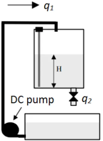
The considered system consists of two tanks (one of them is a buffer tank), a valve, a level sensor, a pipe system and a pump enforcing a movement of water [5]. The pump is driven by a DC motor, which is controlled by a PWM signal. The valve is positioned manually. The level sensor ensures a feedback loop. This system is presented in Figure 1.
Fig. 1.Simplified controlled system
?Lublin University of Technology, Department of Automatics and Metrology, Lublin, Poland,
email: [email protected]
??AGH University of Science and Technology, Department of Automatics and Biomedical Engineering, Krakow,
Poland, e-mail: [email protected], [email protected], [email protected], [email protected]
et. al.
The considered system has the following parameters:
a=0.31m– width
w=0.5m– depth
Hmax=0.4m– maximal height
This system is nonlinear because of the nonlinear function of the valve flow in depen-dence of water level in tank.
2. Modelling
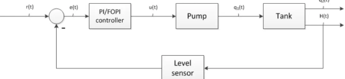
A diagram of a water level automatic control system is illustrated in Figure 2. It is a classic approach to automatic control system. A reference valuer(t)is added to an output signal and it goes to the controller as an error signale(t). The controlling signalu(t)appears at the controller output and controls the pump directly. The pump is a part of controlled system. The loop feedback is realized by the level sensor.
Fig. 2.Diagram of an automatic control system
The control input and output of the system is the water level measured in the tank. The parameters of considered model have been identified by the experiments on the above-mentioned hydro-mechanical system.
The modelling process started with obtaining necessary characteristics. This means: – the water levelHin function of the output sensor voltage,
– the pump efficiencyq1in function of the controlling signalu,
– the valve flowq2in function of the water level in tankH.
First of necessary functions is obtained in the following way: the tank was filled up to a known level and then the value of the output voltage was read (one hundred last samples) and an average value was calculated. This was repeated for a few known water levels. In a result the function of the water level in the tank in dependence of the output sensor voltage was obtained. It is presented in Figure 3.
0.2 0.4 0.6 0.8 1 1.2 1.4 1.6 1.8 2 0 0.05 0.1 0.15 0.2 0.25 0.3 0.35 Voltage U [V] Level H [m] Sensor diagram
Fig. 3.Diagram of the level’s sensor
The approximation of the above characteristic gives a following linear function:
H(U) =0.15616U+0.0069352 (1)
The next important relationship is the pump efficiency in dependence of the controlling signal. The tank was emptied and the valve was closed. Then, the tank was filled up by given time (T =20 s) by the pump controlled with constant PWM signal whereupon the water level was read. This was repeated a few times for different, but constant PWM signals. As a result of those attempts we got set of water level valuesH. Volume of waterV(H)for each of attempts is given by:
V(H) =awH (2)
Finally, the pump efficiencyq1is calculated by the following expression:
q1(H) =V(H)/T (3)
whereT=20 s.
This function is illustrated in Figure 4 and can be approximated with polynomial func-tion:
et. al. 0.2 0.3 0.4 0.5 0.6 0.7 0.8 0.9 1 0.2 0.4 0.6 0.8 1 1.2 1.4 1.6 1.8x 10 −4 PWM signal Flow [m 3/s]
Pump’s efficiency diagram
Fig. 4.The pump’s efficiency diagram
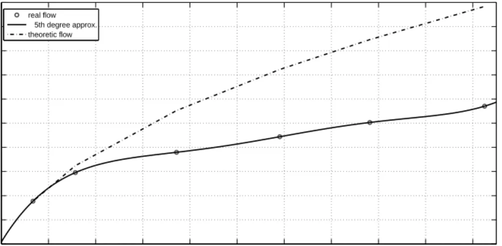
The last necessary function is the valve flow in dependence of the water level. The valve was partly opened and blocked to obtain constant properties of the system and pump was controlled by a constant PWM signal for a long time (min. 5 minutes). The system was brought to a steady state. In this case, pump efficiency equals the valve flow. The function of pump efficiency is known (Fig. 4), so executing the above-mentioned attempts for different PWM signals gives a possibility to get the valve flow in the dependence of the water level, see Figure 5, pointed data.
0 0.02 0.04 0.06 0.08 0.1 0.12 0.14 0.16 0.18 0.2 0.02 0.04 0.06 0.08 0.1 0.12 0.14 0.16 0.18 0.2 0.22 Level [m] Flow [m 3/s] Valve’s flow real flow 5th degree approx. theoretic flow
One can expect: Q2=c r pw b +Hg− pz b (4) where:
pw– a pressure affecting the water’s surface,
pz– an external pressure,
b– a fluid specific weight,
H– a fluid column height,
g– the gravity force,
c– a constant.
Let us considerpw=pz, therefore, one can write:
q2(H) =c2·
√
H (5)
However, the obtained characteristic does not fit to a theoretic diagram, see Figure 5, so one can conclude that the valve’s flow isn’t laminar. The fifth order polynomial approximation seems to be a better representation:
q2(H) = 4093·H5−2479·H4+564,9·H3−59.99·H2+3.231·H+0.0216
The differential equation of the considered system is:
dH
dt =
1
B ·(q1 −q2(H)) (6)
where:
B=a·w– the water’s surface,
q1– the pump efficiency,
q2(H)– the valve flow.
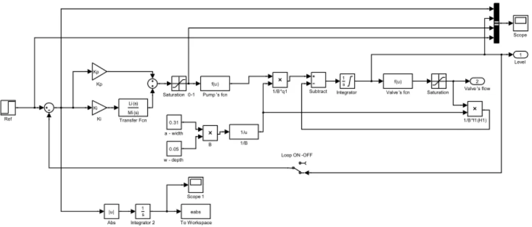
The model of the controlled object and the controller is presented in Figure 6. There is a saturation added because of the limited volume of the tank.
Both the real system and the numerical model are nonlinear because of the nonlinearity in two of tree obtained system parts’ functions. Controllers have been designed on the grounds of a reference point which has been chosen (H0=0.1 m).
et. al. Valve 's flow 2 Level 1 w - depth 0.05 a - width 0.31 Valve 's fcn f(u) Transfer Fcn Li (s) Mi (s) To Workspace eabs Subtract Scope 1 Scope Saturation 0-1 Saturation Ref Pump 's fcn f(u) Loop ON -OFF Kp Kp Ki Ki Integrator 2 1 s Integrator 1 s B Abs |u| 1/B*q1 1/B*f1(H1) 1/B 1/u
Fig. 6.Controlling system numerical model
3. Controlling methods
The non-integer order PIλ controller is a simplified PIλDµ and is described by an
equa-tion (7):
GFOPI(s) =Kp+Ki
1
sλ (7)
whereKp,Kiandλ denote proportional gain, integral gain and integral order respectively.
The comparison has been conducted using the following performances: – steady state error cancellation,
– integral absolute error minimization.
In order to compare the controlling quality of two types of controllers we decided to choose the optimisation method, which gave good results in previous research, it is the sim-ulated annealing [1, 2] method. This minimization method is able to find a global minimum of an objective function. In this case, the integrated absolute error has been chosen as the objective function (8).
This minimization method is able to find a global minimum of an objective function. In this case, the integrated absolute error has been chosen as the objective function (8).
IAE=
t
Z
0
|e(t)|dt (8)
Our purpose is to find the minimum of the objective function for both of the controllers using numerical models of the control system and a real-time simulation results.
In Figure 6 the considered system’s model with the non-integer order PIλ controller is
presented. If we setλ=1,this controller becomes the traditional PI controller. An optimisation
process is made by the simulated annealing method using the parameters from Table 1. Table 1
The parameters of the optimisation
Parameter PI FOPI Description
Ts 100 s 100 s Simulation time
Kpmin 1 1 Minimum proportional coefficient
Kimin 0 0 Minimum integral coefficient
λmin 1 0.1 Minimum integrator’s order
Kpmax 200 200 Maximum proportional coefficient
Kimax 200 200 Maximum integral coefficient
λmax 1 0.9 Maximum integrator’s order
Ref 0.1m 0.1m Reference value (H0)
Umin 0 0 Minimum controlling signal
Umax 1 1 Maximum controlling signal
Hmax 0.35 m 0.35 m Maximum water’s level
N – 5 Oustaloup’s approximation order
ωmin – 10−6 Minimum approximation frequency
ωmax – 102 Maximum approximation frequency
There are two variables of the optimisation method in the PI controller case, those are a proportional coefficientKpand an integral coefficientKi. In the case of the non-integer order
PIλ controller there are three variables, two first same as before and
λ as the third one. The
non-integer order integrator is numerically approached using an Oustaloup approximation [6, 7]. The Oustaloup continuous integer approximation is given by the equation:
sλ≈K N
∏
i=1 s+ω 0 i s+ωi ,α>0where poles, zeros and gain can be evaluated respectively as:
ω
0
i =ωminωu(2i−1−α)/N ωi=ωminωu(2i−1+α)/N
et. al. ωu= r ωmax ωmin K= ωhα
To find optimal parameters of the controller, the simulated annealing optimization method has been chosen. Simulated Annealing is a minimization technique for solving an unconstrained and a bound-constrained optimization problem, which gives a good results in finding a local minimum. At each iteration of the Simulated Annealing algorithm, a new point is randomly generated. The distance of the new point from the current point is based on a probability distribution (temperature function) with a scale proportional to the temper-ature. The algorithm accepts all new points that lower the objective function value, but also, with a certain probability, points that raise the objective function value. By accepting points that raise the quality function, the algorithm avoids being trapped in local minima in early iterations and is able to explore globally for better solutions.
The above-mentioned Oustaloup approximation gives satisfactory results within the fre-quency range [1, 2]. Consequently of carried optimisation process the following results are obtained, see Table 2.
Table 2
The results of the optimisation
Coefficient PI FOPI
Kp 189.86 157.143
Ki 0.5308 0.859
λ – 0.8973
4. Experiments
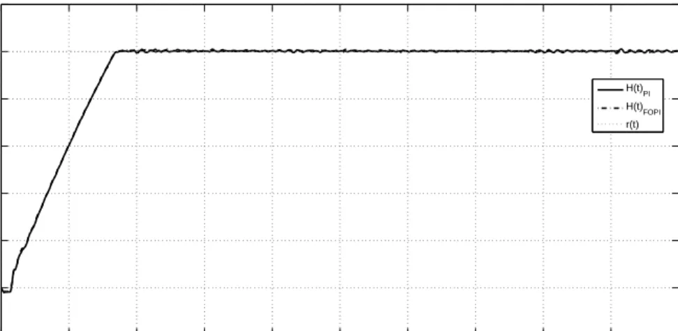
There have been conducted experiments to compare controller performance. A labora-tory workplace that we use consists of a PC with the Matlab/Simulink environment, a RT-DAC process board and a device driver. We added a FIR filter to the real-time controlling system to clear high frequency disturbances from the level sensor. It calculates a moving av-erage with 40 last samples. Controller performance for the hydro-mechanical system have been investigated based on the following experiment. Firstly, we attempted to run the con-trolling process at simulation conditions what is illustrated in Figure 7. There one can see a short delay at the starting point resulting from a short water transportation delay in the pipe from the pump to the tank inlet. A filling process has been running correctly and stable till the water level reached the reference value. Then, the level in the tank has stabilized, but some fluctuation not eliminated in both cases. It is probably effect of water waves in the tank.
Responses of the PI controller and the FOPI controller are very similar. The same can be seen in the error diagram (Fig. 8 and Fig. 9).
0 10 20 30 40 50 60 70 80 90 100 −0.02 0 0.02 0.04 0.06 0.08 0.1 0.12 Time [s] Level [m] H(t)PI H(t)FOPI r(t)
Fig. 7.Step responses for both of the controllers
0 10 20 30 40 50 60 70 80 90 100 −0.02 0 0.02 0.04 0.06 0.08 0.1 0.12 Time[s] Error [m] e(t)PI e(t)FOPI
et. al. 0 5 10 15 20 25 30 35 40 45 50 0.5 0.6 0.7 0.8 0.9 Time [s] IAE IAE(t) PI IAE(t)FOPI
Fig. 9.The Integrated Absolute Error for step response
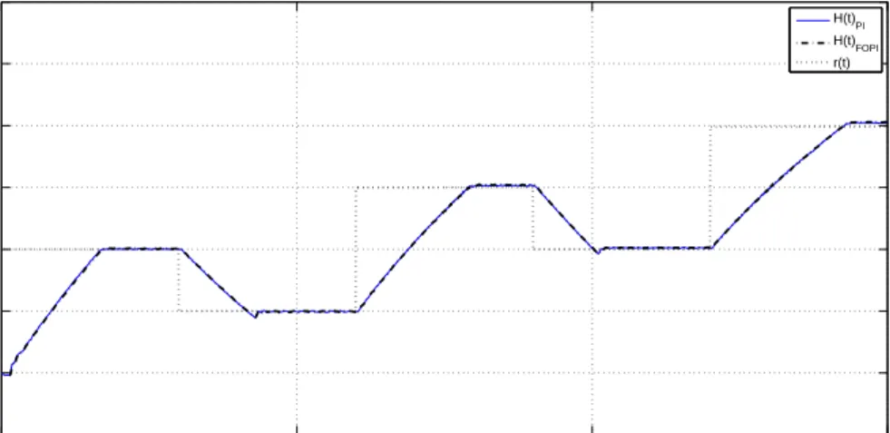
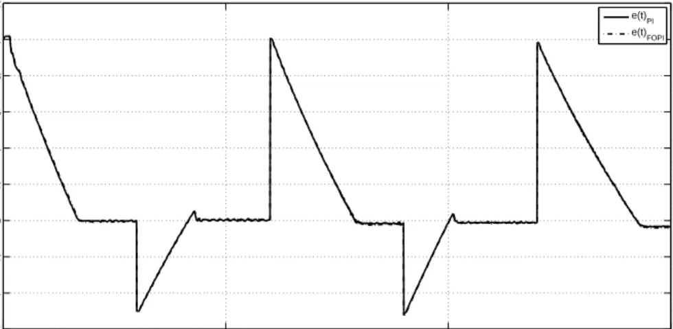
Secondly, the system response for different values of the reference signal has been in-vestigated. One can find transient step responses for 0.1 m, 0.05 m, 0.15 m, 0.1 m, 0.2 m respectively in Figure 10. The reference value changed every 30 seconds. There is a little overshoot during the decreasing the water level and one can see that if the level is higher, the steady state error is larger. Both PI and FOPI controllers offer an almost identical time response. 0 50 100 150 −0.05 0 0.05 0.1 0.15 0.2 0.25 0.3 Time [s] Level H(t)PI H(t) FOPI r(t)
The corresponding error diagrams are shown in Figure 11. The most interesting diagram is presented in Figure 12, where the integrated absolute error is. There is the most visible difference between the integrated absolute error of response with the PI and FOPI controller. Unfortunately, the result of the FOPI controlling is a little worse than the PI controlling result.
0 50 100 150 −0.06 −0.04 −0.02 0 0.02 0.04 0.06 0.08 0.1 0.12 Time [s] Error [m] e(t)PI e(t)FOPI
Fig. 11.The error for several step response
0 50 100 150 0 0.5 1 1.5 2 2.5 3 3.5 Time[s] IAE IAE(t)PI IAE(t)FOPI
et. al.
5. Conclusion
The comparison of two types of PI controllers has been conducted (classical PI controller and non-integer order PIλ controller, FOPI). The ways of developing the two controllers have
been presented and implemented in a hydro-mechanical system. Results show that the non-integer order PIλ controller gives almost as good effects as the traditional PI controller in
such systems but in the same time the non-integer order controller is computationally more complex than the PI controller, therefore using non-integer order PIλ controller to control
even such simple integrating systems proves useless.
Acknowledgements
The work was realised in the scope of project titled „Design and application of non-integer order subsystems in control systems”. The project was financed by the National Sci-ence Centre on the base of decision no. DEC-2013/09/D/ST7/03960.
References
[1] Dziwi´nski T., Bauer W., Baranowski J., Pi ˛atek P., Zagórowska M., Robust Non-integer Order Controller for Air Heating Process Trainer, [in:] Latawiec K.J., Łukaniszyn M., Stanisławski R. (Eds.), Advances in Modelling and Control of Non-integer-Order Systems, 2015, 249–256. [2] Bauer W., Dziwi´nski T., Baranowski J., Pi ˛atek P., Zagórowska M., Comparison of Performance
Indices for Tuning of PIλDµ Controller for Magnetic Levitation System, [in:] Latawiec K.J.,
Łukaniszyn M., Stanisławski R. (Eds.), Advances in Modelling and Control of Non-integer-Order Systems, 2015, 125–133.
[3] Dziwi´nski T., Bauer W., Baranowski J., Pi ˛atek P., Zagórowska M., Robust non-integer order controller for air heater. 19thInternational Conference on Methods and Models in Automation and Robotics, MMAR, 2015.
[4] Bauer W., Baranowski J., Mitowski W., Non-integer order PIαDµcontrol ICU-MM. Theory & Appl. of Non-integer Order Syst. Lecture Notes in Electrical Engineering, 257:295–303, Springer, Heidelberg, 2013
[5] Rosół M., Application of nonlinear control methods for tanks system(in Polish). Pomiary, Au-tomatyka, Kontrola, 7/8:30–34, 2001.
[6] Oustaloup A.,La commande CRONE: commande robuste d’ordre non entierHermes, 1991. [7] Oustaloup A., F. Levron F., Mathieu B., Nanot F.M., Frequency-band complex noninteger
dif-ferentiator: characterization and synthesis. Circuits and Systems I: Fundamental Theory and Applications, IEEE Transactions on, 47(1):25–39, 2000.