Calhoun: The NPS Institutional Archive
Theses and Dissertations Thesis Collection
2013-09
Analysis of decisions made using the analytic
hierarchy process
Tabar, Matthew J.
Monterey, California: Naval Postgraduate School
NAVAL
POSTGRADUATE
SCHOOL
MONTEREY, CALIFORNIA
THESIS
ANALYSIS OF DECISIONS MADE USING THE ANALYTIC HIERARCHY PROCESS
by
Matthew J. Tabar September 2013
Thesis Advisor: Jeffrey A. Appleget Second Reader: Ronald D. Fricker, Jr.
REPORT DOCUMENTATION PAGE
OMB No. 0704–0188Form Approved The public reporting burden for this collection of information is estimated to average 1 hour per response, including the time for reviewing instructions, searching existing data sources, gathering and maintaining the data needed, and completing and reviewing the collection of information. Send comments regarding this burden estimate or any other aspect of this collection of information, including suggestions for reducing this burden to Department of Defense, Washington Headquarters Services, Directorate for Information Operations and Reports (0704–0188), 1215 Jefferson Davis Highway, Suite 1204, Arlington, VA 22202–4302. Respondents should be aware that notwithstanding any other provision of law, no person shall be subject to any penalty for failing to comply with a collection of information if it does not display a currently valid OMB control number. PLEASE DO NOT RETURN YOUR FORM TO THE ABOVE ADDRESS.1. REPORT DATE (DD–MM–YYYY)2. REPORT TYPE 3. DATES COVERED (From — To)
4. TITLE AND SUBTITLE 5a. CONTRACT NUMBER
5b. GRANT NUMBER
5c. PROGRAM ELEMENT NUMBER
5d. PROJECT NUMBER
5e. TASK NUMBER
5f. WORK UNIT NUMBER 6. AUTHOR(S)
7. PERFORMING ORGANIZATION NAME(S) AND ADDRESS(ES) 8. PERFORMING ORGANIZATION REPORT NUMBER
9. SPONSORING / MONITORING AGENCY NAME(S) AND ADDRESS(ES) 10. SPONSOR/MONITOR’S ACRONYM(S)
11. SPONSOR/MONITOR’S REPORT NUMBER(S)
12. DISTRIBUTION / AVAILABILITY STATEMENT
13. SUPPLEMENTARY NOTES
14. ABSTRACT
15. SUBJECT TERMS
16. SECURITY CLASSIFICATION OF: a. REPORT b. ABSTRACT c. THIS PAGE
17. LIMITATION OF ABSTRACT
18. NUMBER OF PAGES
19a. NAME OF RESPONSIBLE PERSON
19b. TELEPHONE NUMBER (include area code)
NSN 7540-01-280-5500 Standard Form 298 (Rev. 8–98)
Prescribed by ANSI Std. Z39.18
30–9–2013 Master’s Thesis 2102-06-01—2104-10-31
ANALYSIS OF DECISIONS MADE USING THE ANALYTIC HIERARCHY PROCESS
Matthew J. Tabar
Naval Postgraduate School Monterey, CA 93943
Department of the Navy
Approved for public release; distribution is unlimited
This thesis analyzes the use of the Analytic Hierarchy Process (AHP) as a decision-making tool. The analysis shows what information can be gained about a military decision-maker who uses the AHP, and how this information can be utilized, permitting U.S. and allied forces to execute efficient and effective military operations. A case study of the AHP decision-making process demonstrates techniques that can be used to garner information about the decision-maker and potentially influence their future decisions.
Analytic Hierarchy Process, Decision Making, Mirror Imaging
Unclassified Unclassified Unclassified UU 69
THIS PAGE INTENTIONALLY LEFT BLANK
Approved for public release; distribution is unlimited
ANALYSIS OF DECISIONS MADE USING THE ANALYTIC HIERARCHY PROCESS
Matthew J. Tabar Lieutenant Commander B.A., University of Cincinnati, 1999 Submitted in partial fulfillment of the
requirements for the degree of
MASTER OF SCIENCE IN OPERATIONS RESEARCH
from the
NAVAL POSTGRADUATE SCHOOL September 2013
Author: Matthew J. Tabar
Approved by: Jeffrey A. Appleget Thesis Advisor
Ronald D. Fricker, Jr. Second Reader
Robert F. Dell
Chair, Department of Operations Research
THIS PAGE INTENTIONALLY LEFT BLANK
ABSTRACT
This thesis analyzes the use of the Analytic Hierarchy Process (AHP) as a decision-making tool. The analysis shows what information can be gained about a military decision-maker who uses the AHP, and how this information can be utilized, permitting U.S. and allied forces to execute efficient and effective military operations. A case study of the AHP decision-making process demonstrates techniques that can be used to garner information about the decision-maker and potentially influence their future decisions.
THIS PAGE INTENTIONALLY LEFT BLANK
Table of Contents
1 Introduction 1
1.1 The Problem of Mirror Imaging . . . 1
1.2 Understanding Decision-making Processes . . . 4
1.3 Thesis Outline . . . 5
2 The Analytic Hierarchy Process 7 2.1 The Process . . . 7
2.2 Literature Review: The Benefits of the AHP . . . 17
2.3 Literature Review: Critiques of the AHP . . . 17
2.4 In Chapter III . . . 21
3 Methodology 23 3.1 Case Study - Description . . . 23
3.2 Thesis - Method . . . 26
4 Analysis Results 29 4.1 Analysis - What Can We Learn from the Decision Results?. . . 29
4.2 Using the Information Gained . . . 33
5 Conclusion 41 5.1 Conclusion . . . 41
5.2 Future Work . . . 41
Appendix: Special Case Study 43
References 45
Initial Distribution List 47
List of Figures
Figure 2.1 Full decision breakdown showing each alternative and its relation to the decision’s factors. . . 8 Figure 2.2 Representation of the basic example decision, showing the breakdown of
the larger decision into its factors and sub-factors. . . 9 Figure 2.3 Representation of the example decision with each factor broken into its
sub-factors. Factor values have been included in parenthesis. . . 12 Figure 2.4 Representation of the example decision broken down to minor sub-factors
with each sub-factor’s contribution to its factor in parenthesis and its overall weight in square brackets. . . 13
Figure 3.1 Representation of the AHP decision construct for the case study. De-picted are the 12 sub-factors that contribute to the four final factors used for the decision, as well as the three alternatives (After Bard and Sousk 1991). . . 27
THIS PAGE INTENTIONALLY LEFT BLANK
List of Tables
Table 2.1 Constructed parameters for the three ships used in the example decision: Which is the best ship? . . . 8 Table 2.2 Matrix of the comparisons of the factors in the overall decision. . . 10 Table 2.3 Matrix of the comparisons of the factors in the overall decision, with the
weight of each factor included. . . 11 Table 2.4 Matrix of the comparisons of the sub-factors in the cost factor, with the
weight of each sub-factor included. . . 11 Table 2.5 Matrix of the comparisons of the sub-factors in thespeedfactor, with the
weight of each sub-factor included. . . 11 Table 2.6 Pairwise comparisons of sub-factors with associated weights. . . 12 Table 2.7 Pairwise comparisons using rounded numbers to conform to Dr. Saaty’s
9 point index. . . 13 Table 2.8 Random Consistency Index as reported by Dr. Saaty (After Saaty 2001). 14 Table 2.9 Example pairwise comparison of alternative’s attribute under a single
fac-tor, herepurchase cost. . . 15 Table 2.10 Relative values for the factors of each alternative in the sample decision,
using simple linear utility functions. . . 16 Table 2.11 Parameters for the ships used in the example problem. . . 16 Table 2.12 Constructed parameters for the three ships used in the rank reversal
exam-ple decision: Which is the best ship? . . . 19 Table 2.13 Calculated global priorities for comparing Ship I and Ship II in the rank
reversal example. Costis normalized to $30M, andSpeedto 30. . . 19
Table 2.14 Calculated global priorities for comparing all three ships in the rank re-versal example. Here,Costis normalized to $30M, andSpeedto 46. . . 20 Table 2.15 Corrected global priorities for comparing all three ships in the rank
rever-sal example. Note, theSpeed criteria is now normalized to 30, the same value as in Table 2.13‘. . . 20
Table 3.1 Pairwise comparisons of the factor in the U. S. Army case study, with the resulting weights given in the far right column. Note, theCI reported in the original article (0.097) corresponds to what this thesis calls a CR
(After Bard and Sousk 1991). . . 25 Table 3.2 Comparisons of each alternative and how it measures up to each factor.
Included are the final tallied results for each alternative’s global priority, and associated rank (After Bard and Sousk 1991). . . 26
Table 4.1 Reported factor weights in the U.S. Army case study (After Bard and Sousk 1991). . . 29 Table 4.2 Reported final scores for the three alternatives in the U.S. Army case study
(After Bard and Sousk 1991). . . 30 Table 4.3 Calculated table of actual pairwise comparisons based on reported weights
(After Bard and Sousk 1991). . . 31 Table 4.4 Table of rounded pairwise comparisons based on reported weights,
show-ing relations to Dr. Saaty’s nine point scale (After Bard and Sousk 1991). 31 Table 4.5 Pairwise comparisons of the three alternatives in the sample decision
(Af-ter Bard and Sousk 1991). . . 31 Table 4.6 Rounded pairwise comparisons of the three alternatives in the sample
de-cision (After Bard and Sousk 1991). . . 32 Table 4.7 Testing for rank reversal by removing the USDCH alternative from the list
of alternatives (After Bard and Sousk 1991). . . 33 Table 4.8 Testing for rank reversal by copying the USDCH alternative from the list
of alternatives (After Bard and Sousk 1991). . . 34 Table 4.9 Result of minimizing resource allocation to a new alternative to achieve a
specified rank. Here the ’cost’ of each factor is equal, and the target rank is 1 (After Bard and Sousk 1991). . . 35
Table 4.10 Result of minimizing resource allocation to a new alternative to achieve a specified rank. Here the ’cost’ of each factor is offset to show how the results can change, and the target rank is still 1 (After Bard and Sousk 1991). . . 36 Table 4.11 Result of a Linear Program designed to misinform a rival using
underesti-mation, claiming that the new alternative is ten percent better in global pri-ority to the current highest global pripri-ority (After Bard and Sousk 1991). 38 Table 4.12 Result of a Linear Program designed to misinform a rival using
overes-timation, claiming the new alternative is twice as good as the old rank 1 (After Bard and Sousk 1991). . . 39
THIS PAGE INTENTIONALLY LEFT BLANK
Lists of Acronyms and Abbreviations
ARMS Advanced Robotic Manipulator System
AHP Analytic Hierarchy Process
COA Courses of Action
FMHR Field Material Handling Robot
FGDO Foreign Government Defense Organizations
MCDM Multi Criteria Decision Making
OR Operations Research
RDTE Research, Development, Test, and Evaluation
RTCH Rough Terrain Cargo Handlers
DoD United States Department of Defense
USDCH Universal Self-Deployable Cargo Handler
THIS PAGE INTENTIONALLY LEFT BLANK
Executive Summary
The Analytic Hierarchy Process (AHP) is a tool used by decision-makers, including many mil-itary ones. The output of the AHP lends itself to analysis to gain much information about the decision-maker’s priorities and thought processes.
The information that can be directly gained from analysis of the output of the AHP include the factors a particular decision-maker relies on to make decisions, and how those factors compare to each other in priority. In addition, the decision itself can be examined for susceptibility to rank reversal. Knowing whether rank reversal is possible in a decision aids in being able to predict the outcome of a decision with new inputs.
Over and above the information that can be directly gained from the output of the AHP, two techniques can be employed, based on the knowledge gained from analyzing the output, in order to exploit AHP decisions. These techniques are overestimation and underestimation. Underestimation allows the determination of the optimal specifications of a new alternative that will cause a rival decision-maker to detrimentally forgo the commitment of additional resources in response to an altered decision.
Overestimation allows the determination of the optimal specifications of a new alternative that will cause a rival decision-maker to needlessly commit resources in response to the altered decision. This can be done while minimizing the required resources needed to produce this new alternative.
Two case studies, one unclassified and one classified, demonstrate the viability the use of these techniques in operational and strategic decision making scenarios.
THIS PAGE INTENTIONALLY LEFT BLANK
Acknowledgements
I would like to thank, first and foremost, Dr. Appleget, for agreeing to undertake this thesis with no specific background in the subject matter. It was a lengthy search to find an advisor, but I’m glad it resulted in a good one.
Next, I would like to thank Dr. Fricker, for helping me make this thesis worthy of submission. I would like to thank my wife, Carah, for editing this thesis. Without her efforts it would sound like a third grader had written it.
I would also like to thank the other staff and my fellow students at the Naval Postgraduate School for making the 10 quarters I have spent in this eight quarter program enjoyable, fruitful, and entertaining.
THIS PAGE INTENTIONALLY LEFT BLANK
CHAPTER 1:
Introduction
This thesis analyzes the use of the Analytic Hierarchy Process (AHP) as a decision-making tool. The analysis shows what information can be gained about a military decision-maker who uses the AHP, and how this information can be utilized, permitting U.S. and allied forces to execute efficient and effective military operations. A case study of a decision made by a military decision-maker through the use of the AHP demonstrates techniques that can be used to garner information about the decision-maker.
1.1
The Problem of Mirror Imaging
In Dien Bien Phu, 1954, the colonial French army, attempting to cut the Vietminh supply lines into Laos, chose artillery sites considered heavily defensible. The sites were surrounded by hills covered in thick jungle. These hills, the French surmised, would be inaccessible to Vietminh artillery, as there was no logistics network in place to move heavy artillery guns to the hilltops. What they did not consider was the Vietminh’s ability to break the guns down and transport them along jungle paths by hand (Windrow, 1998). This ultimately led to the Vietminh outmatching the French in artillery numbers, leading to the French defeat at Dien Bien Phu. This was a historic defeat, since a small, poorly equipped and ill-trained military was able to defeat a first world power. France’s failure at Dien Bien Phu was primarily a result of the cognitive trap of mirror imaging: assuming that the Vietminh would make the same logistics decisions as the French.
1.1.1
What is Mirror Imaging?
Mirror imaging is a form of decision-making in which one party assumes another will act in the same way they would when making a decision. This is commonly seen in military operations when a commander assesses his/her enemy’s options to be the same as their own, and then assumes the enemy will act in the same manner as he/she would. In the example above, the French assessed the surrounding hills to be too rugged for transporting artillery to the top, so they surmised that the Vietminh would be similarly limited. The outcome of the battle illustrates one of the dangers of mirror imaging in a combat situation.
It should be noted that mirror imaging need not occur only between aggressors. Mirror imaging
can have negative impacts on cooperative engagements as well. If partnerAassumes that partner
B will act in a certain way, and plans accordingly, the mutual plan can suffer when B does something different. Mirror imaging stems from a lack of knowledge about the other party’s capabilities or thought processes; the resolution of this effect is to gain a deeper understanding of both. In the cooperation scenario, this is easily achieved by both parties sharing all pertinent information on capabilities and thought processes; which is mutually beneficial and avoids the pitfalls of mirror imaging.
1.1.2
Mirror Imaging Loses Battles
In a competitive situation, mirror imaging is a potentially dangerous situation. A commander may make choices based on erroneous assumptions about their enemy’s actions. In our exam-ple, the French commander decided, "The Vietminh could not get artillery onto those hills, so we do not need to increase our numbers to defend against them." However, the enemy may have different tactics available to them, ones that the commander has never thought of, which will ultimately lead to the commander’s defeat. If the commander had a more complete under-standing of the enemy’s capabilities and thought processes, he would not have relied on mirror imaging, and his actions would have been different. The French commander may have realized, "I assume the Vietminh can get artillery on those hills, so I will increase my numbers and defeat them if they do." Now, using a strategy based on avoiding mirror imaging, the French comman-der can achieve victory. This is a very generalized and simple illustration, but the principle is this: The more information one has about an opponent’s capabilities and thought processes, the more accurately one can predict their actions. This knowledge can lead to a profitable outcome, including military victories in hostile situations.
1.1.3
Mirror Imaging Based Mistakes are Costly and Hard-learned
The common means of learning of the downfall of mirror imaging is to fall victim to it, and reap the bloody benefit of the information gained. This is a costly method, as it means losing battles, personnel, and equipment, for the sake of gaining insight. There is no single solution to mirror imaging; every enemy will have different information or thought processes, and both parties have a vested interest in not letting the other side gain understanding of their capabilities and thought processes. This combination makes mirror imaging an extremely difficult, widespread problem.
This thesis will examine a case study example to offer techniques to combat mirror imaging. This case study will show how analyzing the output of an AHP based decision is a good method
to aid in combating mirror imaging. The AHP lends itself well to analysis, as it is transparent, simple to compute, and easily manipulated. The AHP is a decision-making process that divides a decision into its critical elements, referred to as factors. These factors are then compared to each other by a group of experts to assign a weight to each factor. Finally, each alternative being considered for the decision is then measured according to the factors, and a score is calculated. These scores determine which alternative is considered best. The AHP method clearly delineates what the decision-maker’s thought process and priorities are. Understanding a decision another party has made using the AHP will help commanders make informed decisions about future actions which, in turn, minimizes loss to personnel and equipment, and maximizes battle success.
1.1.4
The History of the Analytic Hierarchy Process
In the late 1960s, Dr. Thomas Saaty, one of the pioneers of Operations Research (OR), was directing research projects for the Arms Control and Disarmament Agency at the U.S. Depart-ment of State. These projects were designed to impleDepart-ment arms control strategies and policies. They brought together many of the country’s top scientists, to formulate ways to reduce arms numbers, and lawyers, to interpret the laws governing arms control. In spite of the talents of the people Dr. Saaty recruited, he was disappointed in the results of the team’s efforts (Foreman & Gass, 2001). Dr. Saaty later recalled the following:
Two things stand out in my mind from that experience. The first is that the theories and models of the scientists were often too general and abstract to be adaptable to particular weapon trade off needs. It was difficult for those who prepared the U.S. position to include their diverse concerns. . . and to come up with practical and sharp answers. The second is that the U.S. position was prepared by lawyers who had a great understanding of legal matters, but [who] were not better than the scientists in assessing the value of the weapon systems to be traded off (Foreman & Gass 1996, p. 5).
In subsequent years, Dr. Saaty developed a tool not just for the scientists and lawyers to use, but useful in a wide range of applications by a variety of professionals. The tool developed, the AHP, is a method of Multi Criteria Decision Making (MCDM). The AHP uses the decision-maker’s opinions to develop a priority list for the factors that make up a decision, as well as how each alternative option weighs against those factors.
The AHP is widely used throughout the world in various fields of study for MCDM. A few examples are: deciding how best to reduce the impact of global climate change (?) (Berrit-tella, Certa, Enea, & Zito 2007), quantifying the overall quality of software systems (Mccaf-frey, 2005), selecting university faculty (Grandzol, 2005), deciding where to locate offshore manufacturing plants (Atthirawong MacCarthy, & Gregory, 2002), assessing risk in operating cross-country petroleum pipelines (Dey, 2003), deciding how best to manage U.S. watersheds (De Steiguer, Duberstein, and Lopes, 2003), and the U. S. Army choosing the best military rough terrain cargo handler (Bard & Sousk, 1990).
1.1.5
AHP in the United States
Aside from a few instances in the U.S. Army, the United States Department of Defense (DoD) does not use the AHP often. This is not due to any perceived flaw in the AHP, but because of a difference in decision-making fundamentals. The DoD prefers the use of methods that leverage its experience in operational matters, using experience as a guide in predicting operations. This leads to the use of simulation, both computer-aided and not, or Courses of Action (COA) devel-opment, which also involves the use of simulation. Simulation has its own set of pros and cons. Among the pros are the ability to consider many options in a single simulation, and to change the input parameters easily in order to view many different situations at once. The con is the pitfall of believing the output of the simulation to be truth and not possibilities. This misplaced belief can still lead to mirror imaging, which we have shown to be a dangerous decision-making method.
Although the DoD does not currently use the AHP often in decision-making, many Foreign Government Defense Organizations (FGDO) do. This difference in decision-making processes between the DoD and FGDO is one which can aid the DoD in gaining an understanding of them. By being aware of FGDO’s processes, the DoD can improve future cooperative or competitive engagements. Therefore, a deep understanding of the AHP and of the decisions that are made using this process is essential in understanding the capabilities and thought processes of many FGDOs. This understanding will aid in both cooperating with our allies and in competing with our adversaries.
1.2
Understanding Decision-making Processes
This thesis does not propose to solve the entire issue of mirror imaging, or to give a cut-and-dried tool to use in analyzing another party’s decisions that applies to every situation. There are, however, several options one can use to counteract some of the issues of mirror imaging in
military scenarios. These include simulating the situation to flesh out all alternatives available to the enemy, producing COAs that cover all possibilities; or analyzing an enemy’s prior decisions in an attempt to predict their actions. The latter option is done most easily with a decision made using the AHP, as it lends itself so well to analysis. Decisions made using the AHP are ideal for analysis because the AHP has a very prescribed methodology, and most of the information that goes into the decision, i.e., the decision-maker’s though process, is presented in the output. It can be difficult to determine these critical pieces of a decision with a simulation or COA development reference, as the inputs to these two methods are not always transparent.
To address the issue of mirror imaging, and present a set of solution techniques, this thesis ex-amines a two case studies of the output of an AHP decision made by military organizations, one unclassified, one classified. This analysis will show what capabilities the military organization has, the alternatives being considered for the decision, and the thought process used to deter-mine what parts of the decision are more or less important. There are two possible outcomes to this type of analysis: either new information is obtained that alters what was known, or old information is confirmed, solidifying preconceived notions. Either way, better understanding is achieved, and mirror imaging is less likely. This information can be used to enhance military efforts by allowing military commanders to better predict their opponents actions, leading to victories.
This thesis will examine a decision made using the AHP in two parts. The first part will be analysis of the decision, the decision hierarchy, the alternative’s hierarchy, and the results, in order to extract what capabilities and thought processes can be gleaned from the decision. The second part of the examination will be an analysis of the ways the decision can be exploited. This analysis will consist of checking the decision output’s resistance to rank reversal, devel-oping a method for inserting an alternative into the output list at a specific point, and using the decision’s mechanic to pick what information about a new alternative will be shared with the decision-maker.
1.3
Thesis Outline
The following chapters are broken down thus: Chapter II covers an in depth history and me-chanics of the AHP, as well as a literature review of its strengths and weaknesses; Chapter III details the selected example problem and the method used for analyzing said problem; Chapter IV presents the results of the analysis; and Chapter V provides conclusions and recommenda-tions.
THIS PAGE INTENTIONALLY LEFT BLANK
CHAPTER 2:
The Analytic Hierarchy Process
The previous chapter established that mirror imaging is a potentially fatal mental trap that decision-makers, especially military decision-makers, can fall into. One defense against this trap is gathering information on an opposing decision-maker’s thought process and capabilities. One way to gather this information is through analyzing the output of the AHP, a process which lends itself well to gathering information on what the user’s priorities and thought processes are. This chapter describes the AHP in detail.
2.1
The Process
In his book,Decision Making for Leaders: The Analytic Hierarchy Process for Decisions in a Complex World, Dr. Thomas Saaty breaks the AHP into five steps, as follows (Saaty, 2001):
• Step 1 - Build a hierarchy
• Step 2 - Make comparisons
• Step 3 - Calculate weights
• Step 4 - Check consistency
• Step 5 - Produce result
Before beginning the in-depth explanation of the AHP, a few terms frequently used in the process need to be defined.
• Hierarchy- The representation of a decision broken down into its constituent pieces, here called factors.
• Factors- The constituent pieces that combine to make a decision. These are broad cate-gories, often lacking detail.
• Sub-factors- The pieces of factors broken down to smaller pieces. As factors are to the decision, sub-factors are to factors. Depending how in depth the decision-maker wants to go, sub-factors can be divided into sub-sub-factors, and etc.
• Weights- The numerical interpretation of how important a factor is to the decision, usually reported as a decimal. All of the factors in a decision will sum up to 1. Sub-factors can have weights as well, representing how important that sub-factor is to its factor.
• Consistency- A measure of how close a matrix is to obeying the rule of consistency, that ifAis twice as important asB, andBis twice as important asC, thenAmust be four times as important asC.
• n - the number of factors or sub-factors used in the final composition of the decision hierarchy.
The best way to describe the AHP is to use an example. For illustration purposes, consider a basic decision of which ship is superior, Ship I, Ship II or Ship III, with the parameters found in Table 2.1:
Table 2.1: Constructed parameters for the three ships used in the example decision: Which is the best ship?
Purchase Cost Sustainment Cost Cruising Speed Top Speed
Ship I $10M $400k 15 25
Ship II $20M $1,000k 15 20
Ship III $30M $2,000k 20 30
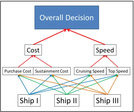
A graphical representation of the decision broken down into factors and sub-factors, along with each alternative, is found in Figure 2.1.
Figure 2.1: Full decision breakdown showing each alternative and its relation to the decision’s factors.
2.1.1
Build a Hierarchy
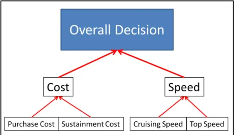
To begin the AHP process, first determine the parts of the decision that contribute to the overall outcome. To do this, divide the decision into broad categories, then subdivide them into smaller pieces. For instance, the ship comparison example decision could be divided into the factors
costandspeed. Thecostfactor could be divided into sub-factorspurchase costandsustainment costandspeedcould be divided into sub-factorscruising speedandtop speed. See Figure 2.1.1 for a graphical depiction of this. For this example, there would ben=4 sub-factors to compare.
Figure 2.2: Representation of the basic example decision, showing the breakdown of the larger decision into its factors and sub-factors.
2.1.2
Make Comparisons
Once the factors and sub-factors have been determined, pairwise comparisons of the factors will need to be made to determine how much each factor contributes to the decision. These comparisons will be made by a panel of subject matter experts chosen by the decision-maker for this purpose. The number and composition of the expert panel is not defined. There can be any number of experts, balancing the experience gained from a large panel, with the ability to reach consensus of small panel. Likewise, diversity in the backgrounds of the panel will increase the knowledge brought to the decision, but could make consensus harder to achieve. There are two ways that the comparisons can be made. The first way is for each expert to assert his/her opinion, and then some method (averaging, weighting, determining means) is used to achieve a single value to represent the group. The second method is for the panel to discuss the decision, and achieve a consensus number together. Whether every expert compiles their own
matrix of comparisons, or all experts decide on a general consensus, the necessary result is a single matrix of pairwise comparisons. In our example this would be a 4 x 4 matrix like the one found in Table 2.7.
In order to make the pairwise comparisons, Dr. Saaty developed a 9-point scale. The scale is based on determining whether one factor compared to another isequally important(1),slightly more important(3),more important(5),greatly more important(7), orabsolutely more impor-tant(9). Values of 2, 4, 6, and 8 are reserved for intermediate values. The reciprocal value is achieved when comparing the factors in the opposite direction, i.e., ifAismore importantthan
B(5),Bcould be said to beless importantthanA(15).
Ultimately, each of the four sub-factors above will need to be compared to each other. There are two ways this can be done. In the first method, the factors ofcostandspeed are compared to each other, followed by comparing each sub-factor under each factor separately. Following the example, definecostasslightly more important(3 on the 9 point scale) thanspeed. The two by two matrix this would produce is shown in Table 2.2. Looking at thecostfactor, let us define
purchase costas between slightlyandmore important thansustainment cost(4 on the 9 point scale). For the speed factor, definecruising speedandtop speedasequally important(1 on the 9 point scale).
Table 2.2: Matrix of the comparisons of the factors in the overall decision.
OVERALL Cost Speed
Cost 1 3
Speed 13 1
The other option to determine each sub-factor’s overall contribution to the decision is to directly compare each sub-factor to every other. This method involves more comparisons, and can become confusing, as a comparison could be made between two very dissimilar sub-factors, leading to an uncertain result. For instance, trying to compare cruising speed to sustainment costwould be difficult, as the two sub-factors are very dissimilar. This second method can also lead to increased inconsistency, as will be discussed below.
2.1.3
Calculate Weights
The calculation of the weight of each factor or sub-factor is an exercise in matrix mathematics. The vector of weights is the normalized eigenvector of the matrix associated with the largest
eigenvalue,λMax, of the matrix. The weights for the pairwise comparison matrix in Table 2.2
are given in Table 2.3.
Table 2.3: Matrix of the comparisons of the factors in the overall decision, with the weight of each factor included.
OVERALL Cost Speed Weight
Cost 1 3 0.75
Speed 13 1 0.25
Tables 2.4 and 2.5 represent the comparisons forcostandspeedrespectively. See Figure 2.1.3 for a graphical depiction of all of weights.
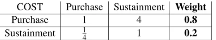
Table 2.4: Matrix of the comparisons of the sub-factors in the cost factor, with the weight of each sub-factor included.
COST Purchase Sustainment Weight
Purchase 1 4 0.8
Sustainment 14 1 0.2
Table 2.5: Matrix of the comparisons of the sub-factors in thespeed factor, with the weight of each sub-factor included.
SPEED Cruising Top Weight
Cruising 1 1 0.5
Top 1 1 0.5
The next step in determining each sub-factor’s contribution to the overall decision is simply to multiply each sub-factor’s value by its corresponding factor’s value. To illustrate, consider the
purchase costsub-factor, where:
• OverallValuePC= The contribution of purchase cost to the overall decision.
• ValuePC= The contribution of purchase cost to the cost factor.
• ValueC = The contribution of cost to the overall decision.
OverallValuePC=ValuePC∗ValueC=0.8∗0.75=0.6 (2.1) The rest of the sub-factors’ overall contributions are tabulated in Table 2.6. In addition, Table 2.6 shows the matrix of pairwise comparison values that result from the calculated weights. These values were calculated by using Equation 2.2. The weights are also graphically depicted in
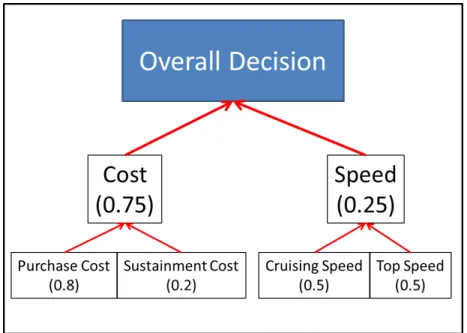
Figure 2.3: Representation of the example decision with each factor broken into its sub-factors. Factor values have been included in parenthesis.
Figure 2.1.3. The calculated weights tell the decision-maker how much each factor contributes to the overall decision. For instance, in our example,pricemakes up 60 percent of the decision of which ship is best.
ComparisonValue= Sub f actorColumnweight
Sub f actorRowweight
(2.2)
For the comparison of the factorsPurchase CostandCruising Speedthis would be 00.125.6 =4.8.
Table 2.6: Pairwise comparisons of sub-factors with associated weights.
Purchase Cost Sustainment Cost Cruising Speed Top Speed Factor
Purchase Cost 1 4 4.8 4.8 0.6
Sustainment 0.25 1 1.2 1.2 0.15
Cruising 0.21 0.83 1 1 0.125
Top 0.21 0.83 1 1 0.125
Returning to the issue mentioned above on the difficulty in comparing each sub-factor to every other, consider this: had that method been chosen to do the comparisons here, an issue would arise, in that not all of the comparisons are whole numbers. To illustrate this, Table 2.6 has been reproduced in Table 2.7, with each comparison value being the rounded value from Table 2.6 to conform to Dr. Saaty’s 9 point scale. The drawback involved with this method will be described
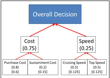
Figure 2.4: Representation of the example decision broken down to minor sub-factors with each sub-factor’s contribution to its factor in parenthesis and its overall weight in square brackets.
in the next section.
Table 2.7: Pairwise comparisons using rounded numbers to conform to Dr. Saaty’s 9 point index.
Purchase Cost Sustainment Cost Cruising Speed Top Speed Factor
Purchase Cost 1 4 5 5 0.612
Sustainment 0.25 1 1 1 0.137
Cruising 0.2 1 1 1 0.13
Top 0.2 1 1 1 0.13
2.1.4
Check Consistency
Once all of the overall weights have been calculated, the next step of the AHP is to check the factor matrix for consistency. Consistency in the matrix is important, because it reflects how precise the result of the process will be. The basic idea of consistency is that for any givennby
nmatrix: Factor 1 · · · Factor N Factor 1 a11 ... a1n .. . ... . .. ... Factor N an1 · · · ann
and for any i,j,k≤n, the equation ai j∗ajk=aik must hold true. Put into plain language, if factorX is two times more important than factor Y, and factorY is two times more important
than factor Z, factorX must be four times more important than factor Z. Inspecting all of the entries in Table 2.6 shows complete consistency. To illustrate the consistency calculations, the matrix in Table 2.7 will now be used.
To calculate inconsistency, Dr. Saaty suggests using the following procedure: First, using the previously determined maximum eigenvalue of the matrix, λmax, calculate the consistency
in-dex,CI, based on Equation 2.3, wheren is the number of factors used in the decision (Saaty, 2001):
CI= λmax−n
n−1 (2.3)
For the matrix in Table 2.7,λmax =4.00623, andn=4, resulting inCI =0.0021. Next, using
the calculatedCI, determine the matrix’s consistency ratio,CRfrom the equation:
CR=CI
RI (2.4)
Here,RI is the random consistency index created by Dr. Saaty and used in all consistency cal-culations. This index is based on the idea that a randomly generatednx nfactor comparison matrix, based on the 9 point scale, will generate a certain amount of inconsistency. For values ofnup to 10, Dr. Saaty randomly generated 500 matrices and calculated their average incon-sistency, to use as a comparison index that he calledRI(Saaty, 2001). The table that Dr. Saaty produced is seen in Table 2.8.
Table 2.8: Random Consistency Index as reported by Dr. Saaty (After Saaty 2001).
n 1 2 3 4 5 6 7 8 9 10
RI 0.00 0.00 0.58 0.90 1.12 1.24 1.32 1.41 1.45 1.49
If the value ofCR is less than 10 percent, i.e. the factor matrix in use has less than 10 percent of the inconsistency found in a random factor matrix, then the matrix is consistent enough and can be used for calculating results. If, however, the CR is higher than 10 percent, the pairwise comparisons should be redone by the expert panel in order to increase the consistency of the final decision. Using Table 2.7’sconsistency index of 0.021 percent, and n=4, it can be seen that the sample problem’s random consistency indexis 0.023 percent, much less than 10 percent. This means that the final decision from this process will produce a result consistent
with the thoughts of the expert panel.
2.1.5
Produce Result
Now that the factors’ weights have been calculated and consistency has been determined to be within acceptable limits, the final step in the AHP is to determine each alternative’s value for each factor. For instance, in the factorpurchase costwe have the values of $10M (Ship I), $20M (Ship II), and $30M (Ship III). The question is: how important is a smaller purchase cost? This is a question that can be answered in several ways. The first way is to submit the alternative’s parameters to the same pairwise comparison process used for the factor’s weights, where ele-ments of the same factor are compared, say purchase cost. This method may be preferred if there are many constraints on the factor, for instance, a $20M budget, or the requirement to buy as many ships as possible with $35M. In order to make the comparisons more logical, the ver-biage of the comparison could be changed toacceptableviceimportant, i.e., a $10M purchase cost is more acceptablethan a $20M purchase cost (5). The result of this would be a list of weights for each alternative’s contribution in each of the factor areas that adds up to 1. Table 2.9 below shows what the comparison matrix would look like forpurchase cost, where:
• $10M is betweenequally as acceptableas andslightly more acceptablethan $20M
• $10M is betweenslightly more acceptableandmore acceptablethan $30M
• $20M is betweenequally as acceptableas andslightly more acceptablethan $10M
Table 2.9: Example pairwise comparison of alternative’s attribute under a single factor, herepurchase cost.
PURCHASE COST Ship I ($10M) Ship II ($20M) Ship III ($30M) Result
Ship I ($10M) 1 2 4 0.57
Ship II ($20M) 12 1 2 0.29
Ship III ($30M) 14 11.5 1 0.14
A second method for obtaining the values is to use a utility function. A utility function allows the decision-maker to set boundaries on the parameters, or to use a scale that is other than linear. This utility function method has a few advantages over the first. One, no more subjective comparisons will have to be made, which can save time and effort on the part of the expert panel. Two, the functions can be reused when new alternatives are submitted, again saving time. For our example problem, a simple normalized linear utility function has been used to convert the ship parameter matrix in Table 2.1 to the utility matrix in Table 2.10.
Table 2.10: Relative values for the factors of each alternative in the sample decision, using simple linear utility functions.
COST SPEED
Purchase Cost Sustainment Cruising Top Ship I 0.67 0.62 0.0 0.33 Ship II 0.33 0.38 0.0 0.0 Ship III 0.0 0.0 1.0 0.67
Once these relative values have been calculated for the alternatives, all that remains is to cal-culate each alternative’s value to the overall decision. This is done by using Equation (2.5) where:
• Value= The alternative’s value in the overall decision.
• Factori= Factori’s contribution to the overall decision.
• AlternativeValuei= The alternative’s relative value for factori.
• k= The number of factors in the decision.
Value=
k
∑
i=1
(Factori∗AlternativeValuei) (2.5)
There are two possibilities when comparing alternatives using the AHP. First, that alternative
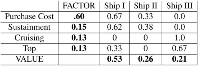
A’s value is equal to alternativeB’s. By the theory of the AHP, this would mean that it makes no difference which alternative is chosen between the two, as they will each satisfy the decision with the same weight. The other possibility is that alternativeA’s value is different than alterna-tiveB’s. The higher value will always determine which alternative is superior. The final values for each alternative in the sample problem are listed in Table 2.11, showing that Ship I is the superior alternative. Note, for this calculation, the weights from Table 2.6, as they are the most consistent.
Table 2.11: Parameters for the ships used in the example problem.
FACTOR Ship I Ship II Ship III Purchase Cost .60 0.67 0.33 0.0 Sustainment 0.15 0.62 0.38 0.0 Cruising 0.13 0 0 1.0 Top 0.13 0.33 0 0.67 VALUE 0.53 0.26 0.21 16
2.2
Literature Review: The Benefits of the AHP
The AHP has many benefits to its use. Primarily these fall under the heading of managing chaos. Specifically, the AHP is a tool that can be used to simplify and synthesize complexity. In addition, the AHP is applicable to a wide range of decisions.
2.2.1
Simplifying Complexity
Dr. Saaty sought, in creating the AHP, a simple way to deal with complexity. Simple enough so that lay people with no formal training could understand and participate. He found one thing common in numerous examples of the ways humans had dealt with complexity over the ages – that was the hierarchical structuring of complexity into homogeneous clusters of factors (Foreman & Gass, 2001).
2.2.2
Synthesis of Complexity
In addition to being able to break a decision down into its constituent factors, the AHP offers an additional benefit, the ability to combine different expert’s analysis. A decision-maker may have multiple different experts working for them, executives in a corporation, commanders in a military, etc., and each expert may have their own analysis of the decision being considered. The AHP allows for diversity in these analyses and makes it possible to combine them into a unified decision, based on the mathematics involved in calculating the weights of factors (Foreman & Gass, 2001, pg. 470).
2.2.3
Applicability
The AHP, due to its comprehensive nature and ability to turn big decisions into a series of small determinations, has a wide range of applications. The AHP can be used for resource allocation, choosing among alternatives, and process engineering, to name a few (Foreman & Gass, 2001, pg. 471).
2.3
Literature Review: Critiques of the AHP
Contrasting the many benefits of the AHP are the flaws that some have found in it. The major flaws that have been noted in numerous articles written since the AHP was first published are its use of the linear 1 to 9 scale, and the issue of rank reversal. These two issues are mildly related, as the inconsistency generated by the linear scale can promote rank reversal.
2.3.1
Linear and Rigid Scale
The first issue commonly reported in literature on the AHP has to do with Dr. Saaty’s choice of a linear 1 to 9 scale for use in the pairwise comparisons. The main issue descends from the possible inconsistency generated from comparisons. For instance, if factorAis determined to beslightly more importantthanB(3), andBis determined to beslightly more importantthanC
(3), then to assure complete consistency,Awould need to be rated asabsolutely more important
than C (3x3 =9). This is a big jump for two factors that are only slightly more important than each other. Following logically, if any two comparisons, A to B and B to C, are more thanslightly more important, the resultant third comparison,AtoC, will induce inconsistency, since 9 is the highest rating possible for any comparison. InSome Comments on the Analytic Hierarchy Process, R.D. Holder proposes the use of an exponential scale to resolve the issue (Holder, 1990, pg. 1073-1074). Essentially, one needs to determine the minimum discernible difference in factors,α. Then, comparisons become exponential factors ofα:
• α0: equally important • α2: slightly more important • α4: more important
• α6: greatly more important • α8: absolutely more important
Now, if factorAis determined to beslightly more importantthanB(α2), andBis determined to
beslightly more importantthanC(α2),Awill be rated asmore importantthanC(α2∗α2=α4),
which makes more sense according to the verbiage descriptions.
Dr. Saaty responded to Mr. Holder’s critiques in the 1991 article "Response to Holder’s Com-ments on the Analytic Hierarchy Process" in the Journal of the Operations Research Society. Dr. Saaty states, "He [Holder] forgets that the AHP is a theory for the human level of coping and not a number-crunching device for measuring a single attribute from zero to infinity" (Saaty, 1991, pg. 911). Dr. Saaty’s point here is that the important thing is that the expert panel be easily able to convey their priorities to the verbiage of the scale, not necessarily that the scale meet a rigorous mathematical definition.
2.3.2
Rank Reversal
The second, and possibly more serious, issue is that the application of the AHP can result in rank reversal. Rank reversal occurs when a new alternative is added to the list of alternatives, or
one of the existing ones is removed, and when the process is re-run, a new order is seen among the alternatives that were included originally. The commonly used scenario is this: the waiter asks if you want chicken or fish, and you reply fish. The waiter then remembers that steak is also available, and you now want chicken. The addition of the third alternative, which does not make it through the decision process as the best option, should not have altered the order of the two existing options.
To illustrate rank reversal, consider this change to the above example: To simplify, the only two criteria for choosing a ship areSpeedandCost, andSpeedis determined to be 40 percent of the decision,Cost60 percent, and each ship’s value are as listed in Table 2.12.
Table 2.12: Constructed parameters for the three ships used in the rank reversal example decision: Which is the best ship?
Cost Speed (0.40) (0.60) Ship I $20M 30 Ship II $30M 20 Ship III $10M 46
To simplify the math, comparisons of ships are done by dividing theCostorSpeedof each ship in the comparison by the highest value in the comparison. If Ship I and Ship II are compared without Ship III, the result would look like Table 2.13. Note that Ship I is considered superior to Ship II.
Table 2.13: Calculated global priorities for comparing Ship I and Ship II in the rank reversal example.
Cost is normalized to $30M, andSpeed to 30.
Cost Speed Global (0.40) (0.60) Priority Ship I 0.67 1.00 0.867
Ship II 1.00 0.67 0.800
If all three ships are compared, the result would look like Table 2.14. Now Ship II is superior to Ship I. This is an example of rank reversal.
Table 2.14: Calculated global priorities for comparing all three ships in the rank reversal example. Here,Cost is normalized to $30M, and Speed to 46.
Cost Speed Global (0.40) (0.60) Priority Ship I 0.67 0.65 0.657
Ship II 1.00 0.43 0.660
Ship III 0.33 1.00 0.733
Many papers and articles have been written about this rank reversal phenomenon, on both sides of the discussion. Again, it is Mr. Holder who gives valuable insight to the problem:
The problem of rank reversal arises because of the insistence that score vectors are normalized, either so that components sum to unity or so that the largest component is unity, before composition with weights, and because weights are elicited without reference to scales for performance against criteria. (Holder 1990, p. 1075)
When the attributes of the alternatives are scored, and those scores are normalized, they will, for instance, be on a zero to one scale. When a new option is introduced, that option, if it falls outside of the previous scale, will change the old scale. This can result in rank reversal, as seen in the above example, if the AHP is not used properly. The best way to fix this issue is to avoid changing the scale. If a new alternative is inserted into the process, it should be rated on the original scale, even when above or below the scale. In the rank reversal example this would mean using Table 2.15 as the corrected ranking.
Table 2.15: Corrected global priorities for comparing all three ships in the rank reversal example. Note, theSpeed criteria is now normalized to 30, the same value as in Table 2.13‘.
Cost Speed Global (0.40) (0.60) Priority Ship I 0.67 0.65 0.867
Ship II 1.00 0.43 0.800
Ship III 0.33 1.00 1.513
2.4
In Chapter III
In the next chapter, a sample decision that uses the AHP will be presented. In addition, the method by which this thesis will analyze the decision will be examined in detail.
THIS PAGE INTENTIONALLY LEFT BLANK
CHAPTER 3:
Methodology
To illustrate information that can be gained by analyzing the output of an AHP decision, this thesis looks at two real-world case studies. The first is a classified case study, covered in Ap-pendix A. The second, discussed here, is based on a 1990 articleA Tradeoff Analysis For Rough Terrain Cargo Handlers Using The AHP: An Example Of Group Decision Making, in which Dr. Jonathan Bard and Dr. Stephen Sousk compared three Rough Terrain Cargo Handlers (RTCH) for the U.S. Army. The evaluation team in this case study consisted of five managers and en-gineers from the Belvoir Research, Development and Engineering Center in Fort Belvoir, VA. The team worked with an objective hierarchy that contained 12 attributes (Bard & Sousk, 1990).
3.1
Case Study - Description
In the 1990s, the U. S. Army was making an effort to reduce risk and boost the productivity of material handling crews. At the time the article was written, the U. S. Army was using three different-sized rough terrain forklifts with maximum lifting capacities of 4,000 lbs., 6,000 lbs., and 10,000 lbs. each.
These vehicles were similar in design and performance to those used by industry, and, at best, could reach speeds of 20 mph. For the most part, this meant that the fleet was not self-deployable; i.e., it could not keep pace with a convoy on most surfaces. As a consequence, additional transportation resources were required for relocation between job sites. This re-striction severely limited the unit’s maneuverability and thus survivability on the battlefield. Additionally, cargo handling personnel had issues related to safety in hazardous nuclear, bi-ological and chemical environments. Although protective gear was available, the operators’ effectiveness was severely hampered by its use. Heat exhaustion, vision impairment, and the requirement for frequent gear changes were the most commonly cited problems (Bard & Sousk, 1990).
At the time, the U.S. Army was investigating the use of robotics to perform many of the dan-gerous and labor-intensive functions normally undertaken by enlisted personnel. To this end, a number of robotics programs were initiated: developing a Universal Self-Deployable Cargo Handler (USDCH) at Belvoir Research, Development, and Engineering Center; developing a
Field Material Handling Robot (FMHR) for the Human Engineering Laboratory, and prototyp-ing an Advanced Robotic Manipulator System (ARMS) for the Defense Advanced Research Projects Agency (Bard & Sousk, 1990).
3.1.1
Case Study - Hierarchy
The team of experts assembled for this decision identified four dominant root factors, with 12 sub-factors that contributed to the overall outcome. The root factors and sub-factors are listed here:
1. Performance
• Mission Objectives: How well does the alternative successfully complete the mis-sion?
• Reliability, Availability, and Maintainability (RAM): How well does the alternative meet military requirements and standards for RAM?
• Safety: How well does the alternative protect the crew? 2. Risk
• System Integration: How well does the alternative sync with other machinery?
• Technical Performance: How does the alternative’s technical specifications (speed, lift capability, etc.) compare to the requirements of the mission?
• Cost Overrun: How likely is the alternative to have a cost overrun?
• Schedule Overrun: How likely is the alternative to have a schedule overrun? 3. Cost
• Research, Development, Test, and Evaluation (RDTE): How much is RDTE ex-pected to cost for the alternative?
• Life-Cycle Cost: What is the expected life cycle cost of the alternative? 4. Program Objectives
• Implementation Timetable: How soon can the alternative be operational?
• Technological Opportunities: What new technologies could be developed in con-junction with the alternative?
• Acceptability: How well is the program accepted, by both user and maker?
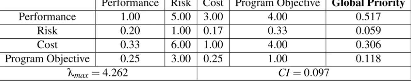
To simplify the process, the experts were only asked to compare the 4 root factors for the process hierarchy. Table 3.1 re-creates the resulting pairwise comparison matrix as reported in the original article (Bard & Sousk, 1990). In order to validate the process that was used in the article, the data given for the pairwise comparisons were used to calculate the global priority
weights, λmax, Consistency Index, CI, and Consistency Ratio, CR. A minor discrepancy was
found in the article’s reported value of 0.097 for the CI, which corresponds to this author’s calculated value of CR. This makes no difference to the integrity of the reported results in the article.
3.1.2
Case Study - Alternatives
According to Drs. Bard and Sousk, in using the AHP to choose amongst alternatives, the Army’s process would result in a vehicle that would be:
• able to substitute for the existing 4,000 lb., 6,000 lb., and 10,000 lb. forklifts, while maintaining current material handling capabilities;
• capable of unaided movement (self-deployability) between job sites at convoy speeds in excess of 40 mph;
• capable of determining if cargo is contaminated by nuclear, biological, or chemical agents;
• capable of handling cargo in all climates, and under all contamination conditions;
• transportable by C-130 and C-141B aircraft;
• operable in the near term as an expandable semi-autonomous man-machine system;
• capable of robotic cargo engagement; and,
• remotely operable from up to one mile away (Bard & Sousk, 1990).
To this end, three alternatives were chosen (Bard & Sousk, 1990) for the analysis:
1. Baseline - The existing system, the 4,000, 6,000, and 10,000 lb rough terrain forklifts augmented with a 6,000 lb variable reach vehicle.
2. Upgraded System- The baseline models upgraded to be self-deployable.
3. USDCH- A teleoperable, robotic-assisted USDCH with micro-cooling for the protective gear, and the potential for full autonomy.
Table 3.1: Pairwise comparisons of the factor in the U. S. Army case study, with the resulting weights given in the far right column. Note, the CI reported in the original article (0.097) corresponds to what this thesis calls aCR (After Bard and Sousk 1991).
Performance Risk Cost Program Objective Global Priority
Performance 1.00 5.00 3.00 4.00 0.517 Risk 0.20 1.00 0.17 0.33 0.059 Cost 0.33 6.00 1.00 4.00 0.306 Program Objective 0.25 3.00 0.25 1.00 0.118 λmax=4.262 CI=0.097 25
A graphical depiction of the decision process is given in Figure 3.1.2.
3.1.3
Case Study - Results
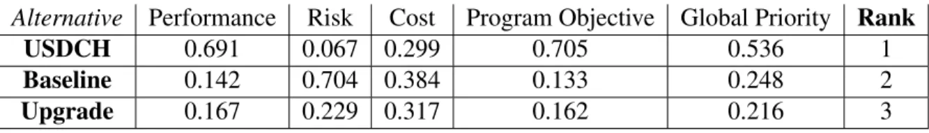
The three alternative cargo handlers were compared under each of the four factors (Perfor-mance, Risk, Cost, and Program Objective) to provide the comparison matrix reproduced in Table 3.2. Note that the values in each column total to one, indicating that these reported values are normalized. Included in Table 3.2 is also the Global Priority and Rank for each alternative, which is the final result of the AHP.
3.2
Thesis - Method
To garner useful information from this case study, the following was done:
• A comparison matrix was generated based on the article’s calculated weights, to show the true comparisons used in the decision.
• A comparison matrix was generated based on the article’s calculated results, to show how the alternatives compare to one another.
• Each alternative was removed from the list to test for rank reversal.
• A fourth alternative was added to the list of alternatives to test for rank reversal.
• A linear program was employed to show how a new alternative can be inserted anywhere into the list of alternatives with minimized resource allocation.
In addition, this thesis extrapolated the techniques above to illustrate how they can be used to the benefit of the side doing the analysis.
Table 3.2: Comparisons of each alternative and how it measures up to each factor. Included are the final tallied results for each alternative’s global priority, and associated rank (After Bard and Sousk 1991).
Alternative Performance Risk Cost Program Objective Global Priority Rank
USDCH 0.691 0.067 0.299 0.705 0.536 1
Baseline 0.142 0.704 0.384 0.133 0.248 2
Upgrade 0.167 0.229 0.317 0.162 0.216 3
Figure 3.1: Representation of the AHP decision construct for the case study. Depicted are the 12 sub-factors that contribute to the four final sub-factors used for the decision, as well as the three alternatives (After Bard and Sousk 1991).
THIS PAGE INTENTIONALLY LEFT BLANK
CHAPTER 4:
Analysis Results
For the results of the classified case study, refer to Appendix A. The analysis of the unclassified case study described in Chapter III netted two basic results. First, it allowed us to gain insights into the decision-maker’s thoughts, either to verify preexisting assumptions, or to establish new ones. Second, the analysis allowed us to find ways to use the information gained to our advan-tage. This chapter details these two aspects. For the purpose of this case study, this author will assume the role of a manufacturer (Company A) who is competing with another manufacturer (Company B) to get the U.S. Army to buy its cargo handler model, and will use analysis of the decision presented in Chapter III as a means to further that end.
4.1
Analysis - What Can We Learn from the Decision
Re-sults?
The AHP lends itself well to gleaning information about the decision-maker who uses the pro-cess. First, the decision-maker’s priorities are laid out in the reported factor weights and final results. In addition, mathematical manipulation of these numbers yields a true comparison ma-trix showing precisely how each of the factors or alternatives compare to each other, in the eyes of the decision-maker. Finally, the results can be tested for susceptibility to rank reversal; this is an important aspect of using the decision to one’s advantage, as understanding of susceptibility to rank reversal can aid in manipulating future decisions given additional inputs.
4.1.1
Priorities
The basic concept of the AHP is to distill the priorities of a panel of subject matter experts into a single vector of weights. The weight vector from the U.S. Army case study appears in Table 4.1.
Table 4.1: Reported factor weights in the U.S. Army case study (After Bard and Sousk 1991).
FACTOR WEIGHT Performance 0.517 Cost 0.306 Program Objective 0.118 Risk 0.059 29
Some basic information can be learned just from inspecting this vector. First, the priority order of the factors is self evident. Here, performance is most important, and risk is least. As a manufacturer, this will lead Company A to spend more resources in an important area like
performancein order to increase perceived overall quality in the eyes of this decision-maker. Additionally, the final output of the AHP, the result vector, is itself a list of priorities presented by the decision-maker. Table 4.2 shows the result vector from the U.S. Army case study. These priority lists are very basic and quite easily attained, and it is good to keep in mind that these are an intrinsic part of the AHP that will be available from every decision made using that process.
4.1.2
True Comparisons
The next step in getting insight into a decision-maker’s mind is to determine just how each factor or alternative compares to its peers. This is done by creating a matrix similar to Table 3.1, but instead of using subjective opinions to create the values, the value is calculated using the weight vector in Table 4.1 and the Equation 4.1.
ComparisonValue=ColumnFactorWeight
RowFactorWeight (4.1)
The resulting matrix is given in Table 4.3. To show the result as it conforms to Dr. Saaty’s nine point scale, the values have been rounded in Table 4.4.
From these tables it can be seen that, according to the experts chosen by the U.S. Army for this decision:
• Performance is betweenequally importantandslightly more importantthan Cost
• Performance is betweenslightly more important andmore important than Program Ob-jective
Table 4.2: Reported final scores for the three alternatives in the U.S. Army case study (After Bard and Sousk 1991). ALTERNATIVE SCORE USDCH 0.536 Baseline 0.248 Upgrade 0.216 30
Table 4.3: Calculated table of actual pairwise comparisons based on reported weights (After Bard and Sousk 1991).
Performance Cost Program Objective Risk
Performance 1.00 1.69 4.38 8.76
Cost 0.59 1.00 2.59 5.19
Program Objective 0.23 0.39 1.00 2.00
Risk 0.11 0.19 0.50 1.00
Table 4.4: Table of rounded pairwise comparisons based on reported weights, showing relations to Dr. Saaty’s nine point scale (After Bard and Sousk 1991).
Performance Cost Program Objective Risk
Performance 1 2 4 9
Cost 12 1 3 5
Program Objective 14 13 1 2
Risk 19 15 12 1
• Performance isabsolutely more importantthan Risk
• Cost isslightly more importantthan Program Objective
• Cost ismore importantthan Risk
• Program Objective is betweenequally importantandslightly more importantthan Risk This is valuable information that is used to build a picture of how this decision-maker thinks. For instance it can be asserted from this information, that the U.S. Army’s panel of experts considers the likelihood of a manufacturer’s cost overrun (risk) to be negligibly important when compared to the a cargo handler’s operational performance (performance). As a manufacturer, Company A may decide to forgo careful consideration of the cost of the cargo handler manufacturing process because the U.S. Army considers that to be of low importance.
This same process of turning the vector into a list of comparisons can be done with the alterna-tives in the decision as well. The pairwise comparisons for the alternaalterna-tives appear in Table 4.5, with the rounded form in Table 4.6.
Table 4.5: Pairwise comparisons of the three alternatives in the sample decision (After Bard and Sousk 1991).
USDCH Baseline Upgrade USDCH 1.00 2.16 2.48
Baseline 0.46 1.00 1.15
Upgrade 0.40 0.87 1.00
Table 4.6: Rounded pairwise comparisons of the three alternatives in the sample decision (After Bard and Sousk 1991).
USDCH Baseline Upgrade
USDCH 1 2 2
Baseline 12 1 1
Upgrade 12 1 1
Again, from these numbers it is seen that:
• The USDCH is betweenequally acceptableandslightly more acceptablethan the Base-line model.
• The USDCH is between equally acceptable and slightly more acceptablethan the Up-graded model.
• The Baseline model isequally acceptableas the Upgraded model.
As a competing manufacturer, Company A now has an idea of how well its cargo handler will have to perform to make it competitive. In addition, Company A can begin to build a picture of how hard it will be to make one that ismore acceptablethan the USDCH, the current favorite.
4.1.3
Rank Reversal Testing
The potential for rank reversal in a decision is important to know. If the potential is evident, a process can be developed to exploit this weakness. If the potential is not present, the intro-duction of new alternatives to the decision will produce predictable results. Knowledge of the potential for rank reversal, therefore, is a valuable tool if one is trying to alter the decision to one’s advantage. It allows one side to have some control over another side’s decision-making process. Recall from Chapter II that there are two general ways to induce rank reversal: remov-ing an alternative, and addremov-ing an alternative. These methods will both be explored for the U.S. Army case study decision.
Removing an Alternative
The procedure for removing an alternative from the list is simple in a decision with three alter-natives. One alternative is removed, and the two remaining are subject to the same procedure outlined in Chapter II for producing a result. This process is detailed for the removal of the USDCH alternative in Table 4.7. Note, these tables depict two subtables, the top shows what al-ternative was added or removed, and the bottom shows how the new alal-ternative list looks when normalized. For decisions with more than three variables, sets of alternatives would need to be
removed sequentially for full rigorous analysis.
Table 4.7: Testing for rank reversal by removing the USDCH alternative from the list of alternatives (After Bard and Sousk 1991).
Alternative Performance Risk Cost Prgm Obj Global Priority Rank USDCH 0.69 0.07 0.30 0.71 0.536 1 Baseline 0.14 0.70 0.38 0.13 0.248 2 Upgrade 0.17 0.23 0.32 0.16 0.216 3
Renormalized List Performance Risk Cost Prgm Obj Global Priority Rank Baseline 0.46 0.75 0.55 0.45 0.503 1 Upgrade 0.54 0.25 0.45 0.55 0.497 2
This same process was used for the other two alternatives as well, with the result that no rank reversal occurs when any of the alternatives are removed.
Adding an Alternative
The next step in testing for rank reversal is to add an alternative in order to induce reversal. As a manufacturer trying to have an effect on this decision, it would be valuable to be able to change the outcome of the decision, not just in where Company A’s product will fall, but in the order of the other products as well. The common additions to the alternative list that cause rank reversal include adding a copy of each alternative, adding an alternative that consists of the highest or lowest attributes, and an alternative that has attributes of 1.5 on the zero to one scale used for the current alternatives. An example of this for adding a copy of the USDCH alternative is found in Table 4.8, the remaining options can be found in Appendix 2. In order to test for rank reversal with an added alternative, the new list of alternatives will need to be renormalized. Table 4.8 shows both the list of alternatives with the raw new alternative, and the list of alternatives with renormalized values.
Inspection of these tables show that there is no evidence of rank reversal. This decision is, therefore, very resistant to rank reversal. As a manufacturer, Company A can use that knowledge to its advantage by using the predictability of the decision. A method of doing this is outlined in the next section.
4.2
Using the Information Gained
The next step in analyzing this decision, having extracted the information about both the decision-maker’s priorities and the decision’s resistance to rank reversal, is to use the decision to Com-pany A’s advantage as a manufacturer to get the U.S. Army to buy their cargo handler before