Department of Economics
Working Paper Series
Bootstrap Unit Root Tests in Models with GARCH(1,1) Errors
09-001 Nikolay Gospodinov Concordia University Ye Tao
Bootstrap Unit Root Tests in Models with
GARCH(1,1) Errors
Nikolay Gospodinovy Concordia University and CIREQ
Ye Taoz Concordia University
January 2009 Revised: May 2009
Abstract
This paper proposes a bootstrap unit root test in models with GARCH(1,1) errors and establishes its asymptotic validity under mild moment and distributional restrictions. While the proposed bootstrap test for a unit root shares the power enhancing properties of its asymptotic counterpart (Ling and Li, 2003), it o¤ers a number of important advantages. In particular, the bootstrap procedure does not require explicit estimation of nuisance parameters that enter the distribution of the test statistic and corrects the substantial size distortions of the asymptotic test that occur for strongly heteroskedastic processes. The simulation results demonstrate the excellent …nite-sample properties of the bootstrap unit root test for a wide range of GARCH speci…cations.
JEL Classi…cation: C12, C15, C22.
Keywords: Unit root test; GARCH; Bootstrap.
We would like to thank the Editor and two anonymous referees for helpful comments and suggestions. The …rst author gratefully acknowledges …nancial support from FQRSC, IFM2 and SSHRC.
yDepartment of Economics, Concordia University, 1455 de Maisonneuve Blvd. West, Montreal, Quebec, H3G 1M8
Canada; tel: (514) 848-2424 (ext.3935), fax: (514) 848-4536, email: [email protected].
zDepartment of Economics, Concordia University, 1455 de Maisonneuve Blvd. West, Montreal, Quebec, H3G 1M8
1
Introduction
The simultaneous presence of high persistence and conditional heteroskedasticity is a common characteristic of many economic time series. The stark di¤erences between the long-run behavior of nonstationary and stationary processes and their implications for economic analysis led to the development of a large class of unit root tests with good size and power properties. While the limiting theory for possibly unit root processes has been established under fairly general conditions, including some types of time-varying volatility, the explicit modeling of the higher-order dynamics is often expected to improve the e¢ ciency of the conditional mean estimates and the power of the tests. For instance, a strand of literature that emerged recently (Ling and Li, 1998, 2003; Ling, Li and McAleer, 2003; Seo, 1999) derives the asymptotic distributions of unit root tests with GARCH errors and demonstrates the power gains of incorporating the GARCH structure into the testing procedure. The form of the asymptotic distribution of the unit root test in this case is a mixture of a Dickey-Fuller (DF) and a standard normal distribution with a mixing coe¢ cient that depends on the degree of conditional heteroskedasticity. As the degree of conditional heteroskedasticity increases (i.e., the sum of the GARCH coe¢ cients approaches one), the standard normal distribution carries more weight and the corresponding smaller critical values give rise to a more powerful testing procedure. Note that the Dickey-Fuller distribution is still valid in the presence of GARCH errors but it is conservative and provides an upper bound for the critical values.
Despite the non-trivial power gains of the unit root tests with GARCH errors (see, for example, Seo, 1999), the applied work with these tests has been very limited. There are several possible reasons why empirical researchers may …nd these tests not to be particularly appealing. First, they require nonlinear (maximum likelihood) estimation as opposed to OLS estimation for the Dickey-Fuller tests. More importantly, the asymptotic distribution depends on nuisance parameters which involves additional computation for obtaining critical values. Finally, as we show later in the paper, the tests based on asymptotic critical values su¤er from substantial size distortions especially for some GARCH parameter con…gurations that are typically documented in empirical studies with …nancial time series data.
In this paper we propose a bootstrap method for approximating the …nite-sample distributions of unit root tests with GARCH(1,1) errors and establish its asymptotic validity. We extend the
results of Basawa et al. (1989, 1991), Ferretti and Romo (1996), Heimann and Kreiss (1996) and
Park (2003), among others, to unit root models with conditional heteroskedasticity estimated by maximum likelihood (ML). The implementation of the proposed bootstrap procedure is straightfor-ward and is valid under some fairly weak conditions. In particular, we follow Ling and Li (2003) and derive the consistency of the bootstrap distribution assuming …nite second moments and symmetry of the errors. This allows for highly persistent GARCH speci…cations (with sum of the GARCH parameters arbitrarily close to one) that are commonly estimated in the empirical …nance litera-ture. Some related bootstrap results are derived in Gospodinov (2008) in the context of testing for nonlinearity in models with a unit root and GARCH errors.
The …nite-sample results demonstrate the excellent size and power properties of the proposed bootstrap test. While the tests based on asymptotic critical values tend to overreject (in some situations, up to 40-50% at 5% signi…cance level), the bootstrap test is always very close to its nominal size regardless of the degree of conditional heteroskedasticity. Furthermore, the power of the bootstrap test that incorporates the GARCH structure of the model exceeds the size-adjusted power of the standard DF test by a substantial margin when the conditional heteroskedasticity is strong.
The properties of the proposed bootstrap test prove to be of great practical importance for identifying the mean reverting behavior in processes with GARCH structure. In our empirical analysis of several U.S. interest rate processes, we show that the DF test does not provide any evidence against the null of a unit root which has important implications about the long-run properties of the data. In contrast, the bootstrap DF-GARCH test tends to reject convincingly the unit root hypothesis due to its superior power properties. This lends support to the mean reverting speci…cation as an underlying process for interest rate dynamics in many economic and …nance models.
The rest of the paper is organized as follows. The main model and notation are introduced in Section 2. Section 3 describes the proposed bootstrap procedure and derives its asymptotic validity. Section 4 presents a Monte Carlo simulation experiment that assesses the …nite-sample performance of the asymptotic and bootstrap tests and illustrates their usefulness for term structure of interest rates. Section 5 concludes. The proofs of all results in the paper are relegated to the Appendix.
2
Model and Notation
Consider the …rst-order AR process with GARCH(1,1) errors
yt = yt 1+"t (1)
"t =
p ht t
ht = !+ "2t 1+ ht 1;
where = 1and t iid(0;1). This model can be generalized to higher-order AR and GARCH
processes. For simplicity, we present the results for the …rst-order model (1) but the limiting representations and the bootstrap procedure can be extended in a straightforward manner (but with more cumbersome notation) to higher-order processes. We can also allow for non-zero mean and linear trend in yt in which case the analysis is performed on the demeaned or detrended
data. We describe below how the asymptotic and bootstrap procedures need to be modi…ed in the presence of deterministic components.
Let = (!; ; ) denote the vector of the unknown GARCH parameters. The parameter of
interest is and the Gaussian quasi-likelihood function of this model is given by
LT( ; ) = 1 T T X t=1 lt( ; ); (2) where lt( ; ) = 12lnht 12" 2 t
ht: We follow Ling and Li (2003) and assume that the following
conditions are satis…ed.
Assumption 1Assume that
(a) t iid(0;1); E( 3t) = 0,E( 4t) = <1for all t;
(b) =f(!; ; ) : 0< !l ! !u; ;0< l u;0< l u; + <1g;
(c) y0 = 0and h0 is initialized from its invariant measure:
Assumption 1 imposes some very weak moment and distributional conditions on the error term. The standardized errors are assumed to be symmetric iid random variables with a …nite fourth moment. The assumed symmetric distribution of t may appear restrictive but this allows us to
weaken the moment requirements on the error term "t (see Ling and Li, 2003). In particular, the
limiting results and the validity of the bootstrap procedure are derived assuming the existence of …nite second moment of "t which is satis…ed under fairly general conditions on the GARCH
parameters. More speci…cally, the conditions in part (b) ensure thatE("2t)<1 and the processes
fhtg and f"tg are strictly stationary, ergodic and -mixing with exponential decay (Carrasco and Chen, 2002; Francq and Zakoïan, 2006) and allow for strong conditional heteroskedasticity that is typically present in …nancial data. Part (c) speci…es the initialization of the conditional mean and variance functions. Assuming y0 to be …xed at a di¤erent value than zero or to be op(T1=2) does
not a¤ect the limiting results derived below. Similarly, the asymptotic distributions are invariant to the assumption on the initial condition ofh (Lee and Hansen, 1994; Ling and Li, 2003).
By the block diagonality of the Hessian matrix (Bollerslev, 1986; Ling, Li and McAleer, 2003), the conditional mean and variance parameters can be estimated separately without any e¢ ciency loss. LetbLS = (PTt=1y2
t 1) 1(
PT
t=1ytyt 1 )denote the OLS estimator of and note thatT(bLS
1) =Op(1)under Assumption 1. The parameter vector can be estimated from the OLS residuals
b"t=yt bLSyt 1 and the corresponding estimatesbare asymptotically equivalent to the estimates
obtained from the true "t. Then, for some preliminary T-consistent estimator e; the one-step
QMLE estimator of is given by
bM L =e 2 4 T X t=1 @2lt ;b @ 2 3 5 1 =e 2 4 T X t=1 @lt ;b @ 3 5 =e
and (Ling and Li, 2003)
T(bM L 1) = " 1 T2 T X t=1 @2lt( ; ) @ 2 # 1 =1 " 1 T T X t=1 @lt( ; ) @ # =1 +op(1):
The OLS estimator bLS can be used as an initial preliminary estimator. Then, the iterative estimator that updates the estimates ofband bM L until convergence is asymptotically equivalent to the full MLE.
Lett LS=1= (PTt=1y2t 1 )1=2(T 1 PT t=1b" 2 t) 1(bLS 1)andt M L=1 = h PT t=1 @2l t( ; ) @ 2 i1=2 =bM L; =b
(bM L 1)be thet-statistics ofH0 : = 1for the OLS and ML estimators, respectively. Let also)
signify weak convergence, D[0;1]denote the space of real valued functions de…ned on the interval [0,1] that are right-continuous at each point in [0,1] and have …nite left limits, and B1(r) be a
standard Brownian motion on D[0;1]. The following lemma is a restatement of some results in Ling and Li (2003) and Seo (1999).
Lemma 1Suppose that = 1 and Assumption 1 holds. Then, as T ! 1 t LS=1) R1 0 B1(r)dB1(r) R1 0 B12(r)dr 1=2; (3) t M L=1 ) r K F 2 6 4 R1 0 B1(r)dB1(r) R1 0 B 2 1(r)dr 1=2 + p 1 2z 3 7 5; (4) where = 1= pK; E(ht) = 2; K=E(1=ht) + ( 1) 2Pk1=1 2(k 1)E("2t k=h2t); F =E(1=ht) +
2 2P1k=1 2(k 1)E("2t k=h2t)and zis a standard normal random variable distributed independently of B1(r).
Proof See Ling and Li (2003) and Seo (1999).
Several interesting observations emerge from the limiting representations in Lemma 1. The as-ymptotic distribution oft M L=1is a scaled mixture of a Dickey-Fuller and a standard normal random
variables with a mixing coe¢ cient that depends on the degree of conditional heteroskedasticity and non-normality of the errors. In the case of normally distributed errors (K =F), the Dickey-Fuller distribution provides an upper bound for the critical values oft M L=1. As the degree of conditional
heteroskedasticity increases,1 more weight is assigned to the standard normal distribution and the corresponding smaller critical values increase the power of the test. The limiting representations for models with constant and linear trend can be obtained by replacing B1(r) in (3) and (4) by
its demeanedB1(r) R1 0 B1(s)dsand detrended B1(r) R1 0(4 6s)B1(s)ds r R1 0(12s 6)B1(s)ds counterparts, respectively.
Another version of the test standardizes (bM L 1)with the robust variance covariance matrix (Bollerslev and Wooldridge, 1992) h PTt=1@2lt( ; )
@ 2 i 1 PT t=1 @lt( ;) @ 2 h PT t=1 @2l t( ;) @ 2 i 1 ;
evaluated at the ML estimates of and ;whose limiting distribution is given by
R1
0 B1(r)dB1(r)
(R1
0 B12(r)dr) 1=2 +
1Boswijk (2001) derives an approximate expression of in terms of the GARCH parameters as q
(1 )(1 2)
(1 + 2)(1 2+2 2):It is then easy to see that high persistence in the conditional variance ( + near one) is typically associated with low values of .
p
1 2 . This test is expected to have more robust size properties with possibly non-normally
distributed errors although at the cost of moderate power losses for Gaussian errors.
Despite its potential for non-trivial power improvements, the test in (4) has the unappealing property that its asymptotic distribution is non-pivotal and depends on nuisance parameters. In principle, one could tabulate critical values for the test t M L=1
q b
F =Kb on a grid of values for (Seo, 1999), where the nuisance parameters are estimated from the data, although this makes the testing procedure somewhat cumbersome. More importantly, the nuisance parameters involve in…nite sums and estimates of , , and h that enter in a highly nonlinear fashion which could impair the precision with which these quantities are computed. As we demonstrate below, this may lead to severe size distortions of the tests even for large sample sizes. The bootstrap method that we propose in this paper proves to be very useful for approximating the …nite-sample distribution of t M L=1 as it avoids the explicit calculation of the nuisance parameters. In addition to the
substantially improved size properties of the unit root test, the straightforward implementation of the bootstrap o¤ers practical advantages and can be easily extended to processes that accommodate more general seral correlation and conditional heteroskedasticity structure.
3
Bootstrap Approximation
In this section, we propose a bootstrap method for approximating the …nite-sample distribution of the unit root testt M L=1:We start by discussing the bootstrap procedures based on resampling the
symmetrized residuals and generating repeated samples under the null of a unit root. In proving the asymptotic validity of the bootstrap, we …rst verify that the bootstrap samples satisfy the conditions of Assumption 1 and the e¤ect of the initial conditions is asymptotically negligible. Then, we develop a bootstrap invariance principle with conditionally heteroskedastic errors and establish the weak convergence of the bootstrap statistic to the limiting distribution in Lemma 1.
3.1 Description of the Bootstrap Procedure
Let fy1; y2; :::; yTg be a sequence of T observations generated by model (1). As argued above, the
conditional mean and variance parameters of (1) can be estimated separately. Let b= !;b b;b
0
recursively from these estimates for some initial valueh0 and bM L denote the one-step or iterated
MLE of introduced in the previous section.
De…ne the residuals e"t = yt bM Lyt 1: While these residuals could also be constructed
im-posing the null of a unit root ( = 1), we follow Paparoditis and Politis (2003) and compute the residuals using the MLE of which helps to retain the important characteristics of the data and improve the power of the unit root test. We then construct the recentered standardized residuals aset=e"t=
q
bht T 1PTi=1e"i=
q
bhi fort= 1;2; :::; T with empirical distribution function denoted
by FeT( ) =T 1PTt=1I(et ) that is used for resampling. Since the underlying distribution of t is assumed to be symmetric (Assumption 1, part (a)), we need to ensure that the empirical
distribution from which the bootstrap samples are drawn is also symmetric. For this reason, we construct the collection f e1; e2; :::; eTg which is symmetric by construction (Jing, 1995).
The bootstrap procedure for approximating the distribution oft M L=1takes the following steps.
First, draw a random sample f 1; 2; ::: Tg from f e1; e2; :::; eTg with replacement and for initial conditions h0 and y0, construct a bootstrap sample recursively as
ht = !b+ (b+b t21)ht 1 yt = yt 1+pht t:
The bootstrap samplefy1; y2; ::::::yT} is …rst used to get the bootstrap QMLE estimates = (! ; ; ) from "t = yt LSyt 1; where LS = (PTt=1y 2
t 1 ) 1 (
PT
t=1ytyt 1). Then, the
one-step bootstrap QMLE of is obtained as
M L=e " T X t=1 @2lt( ; ) @ 2 # 1 =e " T X t=1 @lt( ; ) @ # =e ,
wheree is a preliminary consistent estimate, typically LS:The iterative bootstrap estimator can
be computed by updating the estimates of and M L until convergence. The estimators and
M L are …nally used to calculate the Hessian
h PT t=1 @2l t( ;) @ 2 i 1
= M L; = and thet-statistic of a
unit root t M L=1= h PT t=1 @2l t( ;) @ 2 i1=2 = M L; = ( M L 1):
This algorithm is repeated B times2 and each time the bootstrap unit root statistic t
M L=1 is
computed. LetP denote the distribution of(y1; y2; :::; yT)conditional on the sample(y1; y2; :::; yT)
2
and GT(x) = P (t
M L=1 x) be the bootstrap distribution of t M L=1: Bootstrap critical values
can be obtained by taking the corresponding quantile ofGT(x)and bootstrap p-values of the unit root test are constructed as B 1PBj=1I(t
M L=1 t M L=1). The procedure can be adapted easily
to models with deterministic components.
3.2 Asymptotic Validity of the Bootstrap
This section analyzes the asymptotic properties of the symmetrized-residual bootstrap procedure. We …rst demonstrate that the bootstrap samples satisfy the conditions of Assumption 1. We also show that the initial values used for generating bootstrap samples do not a¤ect the asymptotic distribution of the test statistic. We then establish the bootstrap invariance principle for partial sums of processes with GARCH errors and prove the weak convergence of the bootstrap unit root test statistic to the asymptotic distribution (4) in Lemma 1.
From the properties of the MLE estimator b and the constraints imposed in the estimation of the GARCH parameters, it is easy to verify that part (b) of Assumption 1 still holds for the bootstrap data generating process. As a result, we focus on establishing if the bootstrap samples satisfy the conditions of parts(a) and (c) of Assumption 1.
Let d2(:) denote the Mallows metric3 of degree2;de…ned asd2(FX; FZ) = inf EjX Zj2 1=2
over all joint distributions for the random variablesXandZwith marginal distributionsFX andFZ.
Also, letFeTsym( ) = (2T) 1PTt=1[I(et )+I( et )]denote the empirical distribution function of the symmetrized recentered residuals f e1; e2; :::; eTgand F be the true distribution of the standardized errors t: We use the Mallows metric d2 to show that the symmetrized empirical
distribution function of the recentered standardized residuals provides a good approximation to the true distribution function and the bootstrap errors satisfy the conditions for establishing the bootstrap invariance principle.
Lemma 2. Let E and V ar refer to the expected value and variance of P ; f tgTt=1 be drawn with replacement from FeTsym( ) and suppose that Assumption 1 holds:Then, (a) d2 FeTsym; F ! 0 as
T ! 1, (b) E("t) = 0, (c) V ar ("t) = 2 as T ! 1, and (d) E ("t)3= 0:
Proof. See Appendix A.2. 3
The bootstrap sequences fhtg and f"tg are constructed for some initial values h0 and 0. Auxiliary Lemma 2 in Appendix A.1 establishes that if 0is drawn fromFeTsym( )andht is initialized from its invariant measure, the bootstrap sequences fhtg and f"tg are strictly stationary and ergodic. Furthermore, Auxiliary Lemma 3 in Appendix A.1 shows that the expected di¤erence (underP ) of partial sums constructed from sequences that start from in…nite past and …nite past tend to zero as T ! 1.
The following lemma demonstrates that di¤erent initial values of ht have no asymptotic e¤ect on the bootstrap procedure.
Lemma 3. De…ne the processes t = 1"t + 2[h"t t ^ ht( "2 t ht 1) Pt 1 k=1^ k 1 "t k] and S[T r] = T 1=2P[tT r=1] t for f0 r 1g, where = ( 1; 2) 0
is a constant vector with 0 6= 0: Let h01
and h02 are two di¤ erent initial values of ht and (ht1; ht2); ("t1; "t2) and ( t1; t2) are bootstrap sequences corresponding to these initial values, respectively.
Then, under Assumption 1 and as T ! 1; (a) E jht1 ht2j ! 0, (b) E j"t1 "t2j ! 0, (c) E p1 T PT i=1"i1 p1T PT i=1"i2 = O T 1=2 ; and (d) E S (1) [T r] S (2) [T r] = O T 1=2 , where S[(1)T r]= p1 T P[T r] t=1 t1 and S (2) [T r]= 1 p T P[T r] t=1 t2.
Proof. See Appendix A.2.
Finally, we show that the bootstrap delivers consistent estimates of the nuisance parameters that enter the limiting distribution of the unit root test.
Lemma 4. Under Assumption 1 and as T ! 1; (a) E (ht)! E(ht), (b) E (1=ht) ! E(1=ht),
(c) K !K;and (d) F !F.
Proof. See Appendix A.2.
Now we can establish the bootstrap invariance principle for partial sums of GARCH processes.
Lemma 5.Under Assumption 1,
0 @T 1=2 [T r] X t=1 "t; T 1=2 [T r] X t=1 2 4"t ht + (1 2 t )hb t t X j=1 bj 1 "t j 3 5 1 A)[W1(r); W2(r)]
for all r 2 [0;1]; conditionally on the sample (y1; y2; :::; yT), where [W1(r); W2(r)] is a bivariate
Brownian motion in D[0;1] D[0;1]with mean zero and covariance matrix =r 0
@ E(ht) 1
1 K
1 A;
where K is de…ned in Lemma 1.
Proof. See Appendix A.2.
The results in Lemmas 2 to 5 provide su¢ cient conditions for the asymptotic validity of the bootstrap procedure. The next theorem shows that the bootstrap approximation to the distribution of thet M L=1 test converges weakly to the limiting distribution in Lemma 1 which implies that the
bootstrap is …rst-order asymptotically correct.
Theorem 1.Under Assumption 1 and the null hypothesis H0 : = 1, for any x2Rand >0;
lim
T!1Pr supx
P (t
M L=1 x) P(t M L=1 x) > = 0;
where P(t M L=1 x) is the limiting distribution (4) of the t M L=1 test in Lemma 1.
Proof. See Appendix A.2.
Theorem 1 implies that the critical and p-values for the unit root test with GARCH errors can be approximated by the proposed bootstrap that avoids the explicit estimation of nuisance parameters. An interesting extension that is beyond of the scope of this paper is to study the power of the bootstrap test under the alternative and show that it converges to the power function of the asymptotic test as in Swensen (2003). Also, while investigating the higher-order accuracy of the bootstrap might be interesting, the bootstrap is not expected to o¤er any asymptotic re…nements since the test statistic is not pivotal.
The next section shows that the asymptotic distribution (4) provides a very poor approximation to the …nite-sample distribution of the unit root test when the degree of conditional heteroskedas-ticity is high. This seems to arise from the imprecise estimation of the nuisance parameters as the conditional heteroskedasticity is close to an integrated GARCH process. In contrast, the size of the bootstrap-based test is near the nominal level across all GARCH parameterizations without any adverse e¤ects on the power.
4
Numerical Illustrations
4.1 Monte Carlo Simulation
This section reports the results from a Monte Carlo experiment that assesses the size and power properties of the asymptotic and bootstrap unit root tests in models with GARCH errors. Repeated sample paths are generated from the following model
yt = yt 1+"t (5)
"t =
p ht t
ht = !+ "2t 1+ ht 1;
where t iid(0;1):We consider three error distributions: Gaussian,tdistribution with 7 degrees of freedom and chi-square distribution with 5 degrees of freedom that are appropriately standardized
to have mean zero and variance one. The sample sizes are T = 200 and 400 and the number of
Monte Carlo replications is 2,000.
The autoregressive parameter takes values of1 and0:92 in evaluating the size and the power of the unit root test, respectively. We also normalize the unconditional variance to be one by setting!= 1 . The performance of the tests is evaluated for di¤erent degrees of conditional
heteroskedasticity that cover the conditional homoskedastic case ( + = 0) and some highly
persistent GARCH speci…cations ( + = 0:999). We consider speci…cations that are typically estimated from …nancial data (for example, ( = 0:399; = 0:6)and ( = 0:199; = 0:8)) as well as speci…cations (large and small , for instance) that are not frequently encountered in economic applications. It should be noted that while all speci…cations satisfy the moment conditionE"2t <1, most of the considered GARCH parameterizations renderE"4t in…nite.
We investigate the empirical size and power performance of the asymptotic test based on the OLS estimator (ASY DF), the DF test with critical values approximated by the wild bootstrap
(BOOT DF), the asymptotic test based on the iterated ML estimator of the GARCH model
(ASY GARCH) and its bootstrap analog (BOOT GARCH) discussed in Section 3. All tests are constructed using demeaned data which is equivalent to including an intercept in the estimated models. In the ML estimation of the GARCH parameters, we impose the restriction + <1.
The GARCH bootstrap generates samples under the null of a unit root by resampling the cen-tered, symmetrized standardized residuals. These samples are used to approximate the distribution of the unit root test with 199 bootstrap replications that delivers the corresponding bootstrap crit-ical values. The asymptotic critcrit-ical values for the test based on the OLS estimator are obtained from the Dickey-Fuller tables. For the asymptotic test based on the ML estimator with GARCH errors, we use the true values of , and to obtain the values of the nuisance parametersF,K
and (by truncating the in…nite sums at a large integer value) and then interpolate the appropriate critical values from Table 3 in Seo (1999).
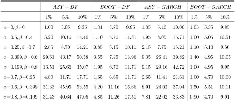
The empirical rejection probabilities under the null of a unit root at 1%, 5% and 10% nominal levels for standard normal errors and sample sizes 200 and 400 are reported in Tables 1 and 2. The asymptotic DF test is well sized in the conditionally homoskedastic case and slightly overrejects for low to moderate degrees of conditional heteroskedasticity. As the GARCH persistence approaches the unit boundary, the size distortions of the DF test are substantial (see also Valkanov, 2005) and are bigger when exceeds :Several recent papers (Beare, 2008; Cavaliere and Taylor, 2008, 2009) have proposed modi…ed unit root test procedures that are robust to the presence of certain types of conditional heteroskedasticity.4 Here, we consider the wild bootstrap approach of Cavaliere and Taylor (2008) who extend the results of Gonçalves and Kilian (2004, 2007) to unit root models with nonstationary volatility. The second column of Tables 1 and 2 presents the results based on the wild bootstrap method. The wild bootstrap reduces the size distortions of the asymptotic DF test but there are still some relative large overrejections when the sum of the GARCH parameters is near unity. This re‡ects the stronger moment requirements on the errors that are needed for establishing the validity of the wild bootstrap (Cavaliere and Taylor, 2008).
The results for theASY GARCH testt M L=1are reported in the third column of Tables 1 and
2. While the size distortions of this test are smaller than those of the DF test, they are still fairly large despite the fact that the ASY GARCH test is designed to handle explicitly the presence 4Some other popular methods for size correction may not be valid or appropriate in our context. For example, using
a robust variance covariance matrix tends to reduce the size distortions (Kim and Schmidt, 1993) but the consistency of this procedure for nonstationary processes has not been formally established. Also, while the resampling scheme that incorporates the GARCH structure of the model can certainly be used for the DF test, it is not obvious why one would employ it for this test and not for the more powerful test based on the ML estimator.
of conditional heteroskedasticity. Substantial overrejections occur when the GARCH speci…cation borders an integrated GARCH process.5
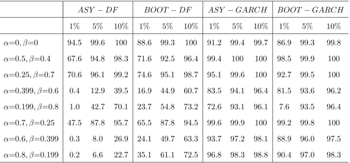
In contrast to the large size distortions of the asymptotic tests, our proposed bootstrap method (last column in Tables 1 and 2) controls the size of the unit root test with GARCH errors uniformly across all GARCH speci…cations and nominal levels. This impressive performance of the bootstrap unit root test is achieved despite the small number of bootstrap replications. Overall, our bootstrap procedure proves to be very e¤ective for correcting the overrejections of the ASY GARCH test. Tables 3 and 4 report the empirical power of the unit root tests with simulated data from model (5) with = 0:92, t N(0;1)andT = 200and 400:The rejection probabilities for the asymptotic
tests (ASY DF andASY GARCH) is size-adjusted power whereas the power of the bootstrap
tests (BOOT DF andBOOT GARCH) is raw power. One interesting observation that emerges
from the results is that the asymptotic DF test is not able to detect any deviations from the null hypothesis when the conditional heteroskedasticity is very strong and T = 200. For example, if ( = 0:6; = 0:399)and ( = 0:8; = 0:199);the size-adjusted power of the DF test is only 6.70% and 7.12% at 10% nominal level and T = 200. Even for the parameterization ( = 0:399; = 0:6)
that is more often encountered in …nancial applications, the power is 9.55% at 10% nominal level. As the sample size gets larger,6 the power of the asymptotic DF test improves but it is still well
below that of theASY GARCH test. Interestingly, the wild bootstrap has better power than its asymptotic analog although some of the power gains are due to the overrejections under the null of a unit root reported in Tables 1 and 2.
The tests that incorporate the GARCH structure of the model su¤er only a small power loss in the conditionally homoskedastic case but o¤er moderate to very large power gains when the degree of conditional heteroskedasticity in the GARCH speci…cation increases. These substantial power 5Our numerical experiments suggest that these overrejections are due to imprecise estimation of the nuisance
parameters 2 =E(ht); E(1=ht)andK as + is close to one. For example, when + = 0:99, the estimates of 2
start to deviate signi…cantly from1and tend to be biased towards 0. The di¤erence becomes even more extreme for + = 0:999and large values of (Gospodinov and Tao, 2009).
6
All computations are performed in GAUSS. The computational time increases roughly 1.5 times when the sample size doubles from 200 to 400. More precisely, the average time withT = 200is 2.2 seconds per Monte Carlo replication while withT= 400;it is 3.3 seconds (2.66GHz Intel Core 2 processor).
improvements, combined with the size correction property of the bootstrap method, illustrate the potential of the ML-based tests to detect the mean reversion in processes with strong conditional heteroskedasticity. The raw power of the bootstrap test is very close, albeit slightly below, the (typically infeasible in practice) size-adjusted power ofASY GARCH. Davidson and MacKinnon (2006) analyze the discrepancy that arises between the rejection probabilities of the bootstrap test and the size-adjusted power of the asymptotic test and suggest possible ways of minimizing it.
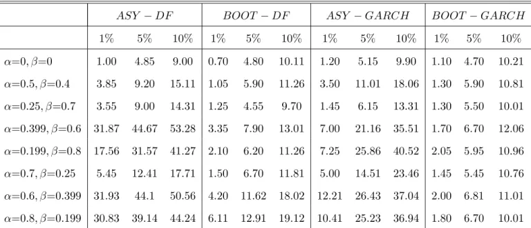
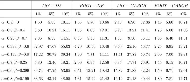
We now turn our attention to the size and power properties of the unit root tests with non-normal errors. Thetdistribution with 7 degrees of freedom is often used in econometric applications to capture the fatter tails of …nancial data at weekly or monthly frequency. The 2 distribution
does not satisfy the symmetry condition in part (a) of Assumption 1 and is used to investigate the sensitivity of the tests to asymmetric errors. While the 2 distribution with 5 degrees of freedom
produces much larger asymmetry than that typically observed in economic and …nancial data, it would be interesting to assess the behavior of the tests for more extreme speci…cations. In this case, we do not symmetrize the residuals as in Section 3.1 and allow the bootstrap procedure to adapt to the shape of the estimated error distribution. To preserve space, we only report the empirical size and power of the tests for T = 200. The results for non-normal errors (Tables 5 and 6 for t7
distribution and Tables 7 and 8 for 2
5 distribution) can be summarized as follows.
The empirical size and power of the asymptotic DF test appears to be fairly similar across the di¤erent error distributions. The bootstrap DF test tends to overreject more for non-normal errors, especially then the sum of the GARCH parameters is near unity (in some cases, the empirical size is close to and above 20% at 10% nominal level). Overall, the wild bootstrap appears to be an e¤ective tool for reducing the large size distortions of the asymptotic DF test although, strictly speaking, it is not theoretically valid for most of the GARCH speci…cations considered in this paper. The performance of theASY GARCH test deteriorates further in the case of 25-distributed errors as predicted by theory. While theBOOT GARCHtest also tends to overreject for asymmetric errors (by 2-3 percentage points at 10% nominal level), it is still very well sized and delivers signi…cant power improvements.
4.2 Testing for a Unit Root in U.S. Interest Rates
The correct speci…cation of the dynamics of interest rates plays an important role in derivative pricing, hedging and term structure modeling. For example, most di¤usion models of spot interest rate that are used for bond valuation impose a mean reverting behavior on the underlying process. Yet, unit root tests for post-war U.S. interest rates rarely reject the null of a unit root which requires that this nonstationarity is taken into account in modeling and long-run forecasting of interest rates. This empirical …nding not only creates some tension between the dynamics of interest rates in theoretical …nance and the speci…cation adopted in practice but it may also cause substantial size distortions in testing the parameters in term structure models (Elliott, 1998).
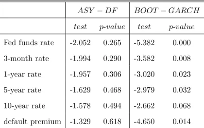
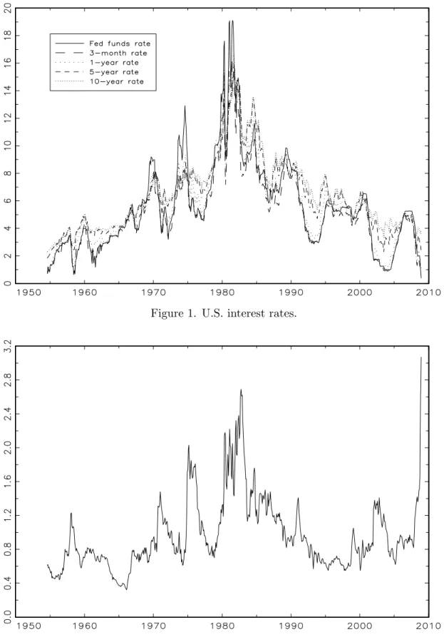
While the conditional heteroskedasticity is a widely documented characteristic of interest rates, the unit root tests typically do not incorporate explicitly the strong GARCH e¤ect into the testing procedure. We re-examine the possibility of a mean reversion in U.S. interest rates using the bootstrap test proposed in this paper. The data employed in the analysis include the Federal Funds rate, 3-month Treasury bill rate (secondary market), 1-, 5- and 10-year Treasury bond yields (constant maturity) and the default premium constructed as the di¤erence between the Aaa and Baa corporate bond yields. The series are annualized rates at monthly frequency covering the period July 1954 - November 2008 and are downloaded from Table H.15 of the Federal Reserve
Statistical Release (http://www.federalreserve.gov/releases/h15/data.htm). The dynamics
of the …ve interest rates and the default premium are plotted in Figures 1 and 2, respectively. The graphs show that all series are characterized by high persistence over the sample period. The short-term interest rates appear to be more volatile than the long-term rates and the dynamics become smoother as the time to maturity increases. Finally, the sum of the estimated GARCH parameters for all interest rates is very close to one which indicates a strong volatility clustering.
The results from the Dickey-Fuller and the GARCH-based unit root tests are reported in Table 9. Since the interest rates do not exhibit any trending behavior, we consider a model that includes an intercept but not a linear trend. The values of the DF statistic for all interest rate processes do not exceed the asymptotic critical values at 5% and 10% signi…cance level (-2.86 and -2.57, respectively). The asymptotic p-values of the DF tests are between 0.27 and 0.62 and provide no evidence against the null of a unit root. This appears to be due to the low power of the DF test
for detecting mean reversion in processes with strong conditional heteroskedasticity reported in our simulation study. The results from our bootstrap test with GARCH errors stand in sharp contrast with this …nding. The bootstrap p-values of theBOOT GARCH test suggest that the null of a unit root can be rejected at 5% signi…cance level for all interest rates except for the 10-year yield whose bootstrap p-value is 0.068. Incorporating the GARCH structure of interest rates into the testing procedure con…rms the substantial power gains documented in the previous section. This rejection of the unit root hypothesis also lends empirical support to the mean reverting di¤usion speci…cation that is typically used in …nancial economics to describe the dynamics of short-term interest rates.
5
Conclusion
This paper proposes a bootstrap test for a unit root in processes with GARCH errors and shows its asymptotic validity under very weak moment and distributional assumptions. The proposed method o¤ers several important advantages over its asymptotic counterpart and the existing tests that do not exploit the information in the conditional variance. First, the test delivers impressive power gains by explicitly incorporating the GARCH structure of the errors, especially for highly persistent GARCH speci…cations with power improvements over the DF-type tests. While the asymptotic counterpart of the test requires the computation of nuisance parameters and su¤ers from relatively large size distortions, the proposed bootstrap procedure is straightforward to implement and appears to control the size uniformly over all possible GARCH speci…cations that guarantee the existence of second moments of the errors. Finally, while generalizing the asymptotic theory to more complicated setups would be quite involved, our bootstrap method can be easily adapted to models with a lag length that goes to in…nity at certain rate, asymmetric errors and di¤erent types of conditional heteroskedasticity (other models from the GARCH class, stochastic volatility models etc.)
References
[1] Basawa, I.V., Mallik, A.K., McCormick, W.P., Reeves, J.H., Taylor, R.L. (1991). Bootstrap-ping unstable …rst-order autoregressive processes.Annals of Statistics 19:1098-1101.
[2] Basawa, I.V., Mallik, A.K., McCormick, W.P., Taylor, R.L. (1989). Bootstrapping explosive autoregressive processes.Annals of Statistics 17:1479-1486.
[3] Beare, B.K. (2008). Unit root testing with unstable volatility. Nu¢ eld College Economics Working Paper No. 2008-06.
[4] Bickel, P.J., Freedman, D. (1981). Some asymptotic theory for the bootstrap. Annals of Sta-tistics 9:1196-1217.
[5] Bollerslev, T. (1986). Generalized autoregressive conditional heteroscedasticity. Journal of Econometrics 31:307-328.
[6] Bollerslev, T., Wooldridge, J.M. (1992). Quasi-maximum likelihood estimation and inference in dynamic models with time-varying covariances. Econometric Reviews 11:143-172.
[7] Boswijk, H.P. (2001). Testing for a unit root with near-integrated volatility. Unpublished man-uscript, Universiteit van Amsterdam.
[8] Carrasco, M., Chen, X. (2002). Mixing and moment properties of various GARCH and sto-chastic volatility models.Econometric Theory 18:17-39.
[9] Cavaliere, G., Taylor, A.M.R. (2008). Bootstrap unit root tests for time series with nonsta-tionary volatility.Econometric Theory 24:43-71.
[10] Cavaliere, G., Taylor, A.M.R. (2009). Bootstrap M unit root tests. Econometric Reviews
28:393-421.
[11] Davidson, R., MacKinnon, J.G. (2000). Bootstrap tests: How many bootstraps? Econometric Reviews 19:55-68.
[12] Davidson, R., MacKinnon, J.G. (2006). The power of bootstrap and asymptotic tests.Journal of Econometrics 133:421–441.
[13] Elliott, G. (1998). On the robustness of cointegration methods when regressors almost have unit roots.Econometrica 66:149-158.
[14] Ferretti, N., Romo, J. (1996). Unit root bootstrap tests for AR(1) models.Biometrika 83:849-860.
[15] Francq, C., Zakoïan, J.M. (2006). Mixing properties of a general class of GARCH(1,1) models without moment assumptions on the observed process. Econometric Theory 22:815-834. [16] Gonçalves, S., Killan, L. (2004). Bootstrapping autoregression with conditional
heteroskedas-ticity of unknown form.Journal of Econometrics 123:89-120.
[17] Gonçalves, S., Killan, L. (2007). Asymptotic and bootstrap inference for AR(in…nity) processes with conditional heteroskedasticity. Econometric Reviews 26:609-641.
[18] Gospodinov, N. (2008). Asymptotic and bootstrap tests for linearity in a TAR-GARCH(1,1) model with a unit root.Journal of Econometrics 146:146-161.
[19] Gospodinov, N., Tao, Y. (2009). Bootstrap unit root tests in models with GARCH(1,1) errors. Working paper 09-001, Concordia University.
[20] Heimann, G., Kreiss J.P. (1996). Bootstrapping general …rst order autoregression. Statistics and Probability Letters 30:87-98.
[21] Jing, B.Y. (1995). Some resampling procedures under symmetry.Australian Journal of Statis-tics 37:337-344.
[22] Kim, K., Schmidt, P. (1993). Unit root tests with conditional heteroskedasticity. Journal of Econometrics 59:287-300.
[23] Lee, S.W., Hansen, B.E. (1994). Asymptotic theory for the GARCH(1,1) quasi-maximum likelihood estimator. Econometric Theory 10:29-52.
[24] Ling, S., Li, W.K. (1998). Limiting distributions of maximum likelihood estimators for unstable autoregressive moving-average time series with general autoregressive heteroskedastic errors.
Annals of Statistics 26:84-125.
[25] Ling, S., Li, W.K. (2003). Asymptotic inference for unit root processes with GARCH (1,1) errors.Econometric Theory 19:541-564.
[26] Ling, S., Li, W.K., McAleer, M. (2003). Estimation and testing for unit root processes with GARCH (1,1) errors: Theory and Monte Carlo evidence.Econometric Reviews 22:179-202. [27] MacKinnon, J.G. (1996). Numerical distribution functions for unit root and cointegration tests.
Journal of Applied Econometrics 11:601-618.
[28] Nelson, D.B. (1990). Stationarity and persistence in the GARCH (1,1,) model. Econometric Theory 6:318-334.
[29] Paparoditis, E., Politis, D.N. (2003). Residual-based block bootstrap for unit root testing.
Econometrica 71:813-855.
[30] Park, J.Y. (2003). Bootstrap Unit Root Test. Econometrica 71:1845–1895
[31] Pascual, L., Romo, J., Ruiz, E. (2000). Forecasting returns and volatilities in GARCH process using the bootstrap. Working paper 00-68, Universidad Carlos III de Madrid.
[32] Seo, B. (1999). Distribution theory for unit root tests with conditional heteroskedasticity.
Journal of Econometrics 91:113-144.
[33] Swensen, A.R. (2003). A note on the power of bootstrap unit root tests. Econometric Theory
19:32-48.
[34] Valkanov, R. (2005). Functional central limit theorem approximations and the distribution of the Dickey-Fuller test with strongly heteroskedastic data.Economics Letters 86:427-433.
A
Appendix: Auxiliary Lemmas and Proofs
A.1 Auxiliary Lemmas
Auxiliary Lemma 1. Under Assumption 1, (a) bht ht=op(1) +O( t) and (b) " 2 t
htbht =Op(1):
Proof. For proof of part (a); see Gospodinov (2008). For part (b) note that "2t
htbht < "2t !!b "2 t 2;
where = minf!;b!g>0. SinceE "2t 2 =
2 2 and
"2t
htbht 0, it is easy to show that
"2t
htbht =Op(1).
Auxiliary Lemma 2. Let ht =!bh1 +P1k=1 ki=1 ^ t i2 + ^ iand "t = t
r b
!h1 +P1k=1 k
i=1 ^ t i2 + ^
i
and suppose that 0 is drawn from FeTsym( ) and the sequence fhtg is initialized from its invariant measure. Then, fhtg and f"tg are strictly stationary and ergodic processes.
Proof. The proof follows directly from Theorem 2 in Nelson (1990).
Auxiliary Lemma 3. Let t = 1"t + 2["ht t ^ ht( "2 t ht 1) Pt 1 k=1^ k 1 "t k] and 0t = 1"t + 2[h"t t ^ ht( " 2 t ht 1) P1 k=1^ k 1 "t k], and denote S[T r] = p1T P[T r] t=1 t and S[0T r] = 1 p T P[T r] t=1 0t for f0 r 1g: Then,E S[T r] S[0T r] !0.
Proof. The proof is similar to that of (4.6) in Lemma 4.2 in Ling and Li (2003). More speci…cally,
E S[T r] S[0T r] p1 T [T r] X t=1 E 2 ht "t2 ht 1 ^ 1 X k=t ^k 1" t k ! 1 p T [T r] X t=1 E p2 ^0 ( t2 1) E ^ 1 X k=t ^k 1"t k p ht c p T [T r] X t=1 1 X k=t ^(k 1)=2 ! = pc T [T r] X t=1 O ^t=2 !0 asT ! 1; wherec is a constant:
A.2 Proofs of Lemmas and Theorems Proof of Lemma 2
part (a): For any 2R,
FTsym( ) = 1 2T 2T X i=1 I( i ) = 1 2T T X i=1 I( i ) + 1 2T T X i=1 I( i ) (6) = 1 2[FT( ) + (1 FT( ))] ! 1 2[F( ) + (1 F( ))] =F( ) asT ! 1
and by the symmetry ofF. Becaused2is a metric,d2 FeTsym; F 2 d2 FeTsym; FTsym 2 +d2 FTsym; F 2 andd2 FTsym; F 2
!0from (6) and Bickel and Freedman (1981). Next, it is easy to show (Pascual
et al., 2000) thatd2(FeTsym; FTsym)2 E ej j
2 6 T PT j=1 ej j 2 +T32 PT i=1 i 2 !0since T 1=2PTi=1 i =Op(1) and T6 PTj=1 ej j 2 = T6 PTj=1 " 2 j hjbhj b h1j=2 h1j=2 2 ! 0 from Auxiliary Lemma 1.
part(b): Note that thekthmoment of the symmetrized residualsfe1;e2; :::;eT; e1; e2; :::; eTg
is given by (2T) 1hPT t=1(et)k+ PT t=1( et)k i =T 1PT
t=1(et)p if p 1 is even and 0 if p is odd.
Then, since f tg is an iid sample from the symmetrized empirical distribution function of the recentered standardized residuals; E ( t) = 0and hence E ("t) = 0:
part (c): Because E ("t) = 0 and t are iidconditionally on the sample, V ar ("t) =E ("t)2 =
E (ht)E ( t)2 and V ar ("
t) = T1
PT
t=1bht T1 PTt=1e 2
t : From part (a) of Auxiliary Lemma 1
and PTt=1 t = Op(1); it follows that that T1 PTt=1 bht ht = op(1) and T1 PTt=1bht p
! E(ht).
Combining this result with T1 PTt=1e2t !p 1, we have V ar ("t)!p 2 asT ! 1:
part(d): SinceE ( t)3= 0by construction, t areiidconditionally on the sample, andT1 PTt=1bht=
Op(1);we obtain thatE ("t)3= 0: Proof of Lemma 3
part (a): By recursive substitution,
ht =!b[1 + t 1 X k=1 k Y i=1 b t i2 +b ] +!b t Y i=1 b t i2 +b h0:
If the two candidate initial values are h01 and h02, then the di¤erence between the corresponding sequencesht1 and ht2 is given by jht1 ht2j=!b
t Q i=1 b 2 t i+b jh01 h02jand E jht1 ht2j=b!jh01 h02jE " t Y i=1 b t i2 +b # =b!jh01 h02j b+b t;
using thatE ( t)2 !1:Since b+b <1by construction,E jht1 ht2j !0 ast! 1.
part (b): Rewrite pht1 pht2 as pht1 pht2 = pht1 ht2 ht1+pht2 ht1 ht2 2!b :Then, E j"t1 "t2j = Eh pht1 pht2 j tji E ht1 ht2 2!b j tj = 1 2jh01 h02j ^ + ^ t E j tj
using thatE ( t)2 !1. SinceE j tj<1 and b+b <1,Ej"t1 "t2j !0 ast! 1.
part (c): Note that
E p1 T T X i=1 "i1 p1 T T X i=1 "i2 p1 T T X i=1 E j"i1 "i2j p1 T T X i=1 1 2jh01 h02j ^ + ^ i E j tj = jh01 h02jE j tj 2pT 1 ^ + ^ T+1 1 ^ + ^ 1 2pT jh01 h02jE j tj 1 ^ + ^ =O p1 T :
part (d): Taking expectations under P of the di¤erence betweenS[(1)T r] andS[(2)T r] yields
E S[(1)T r] S[(2)T r] p1 TE [T r] X t=1 j"t1 "t2j+ p2 TE [T r] X t=1 "t1 ht1 "t2 ht2 +p2^ T [T r] X t=1 E t 1 X k=1 ^k 1"t k1 ht1 t 1 X k=1 ^k 1"t k2 ht2 E ( 2 t 1) = 1I1+ 2I2+ 2^I3:
From part (c) we know I1 =O T 1=2 . Furthermore, I2 = p1TE P[tT r=1] p1h t1 1 ph t2 t 1 b !pTE PT
t=1j"t1 "t2j = O T 1=2 . Using similar arguments, it can be shown (see Gospodinov
and Tao, 2009) that I3=O T 1=2 and, hence, E S[(1)T r] S[(2)T r] =O T 1=2 . Proof of Lemma 4
part (a): As in part (a) of Auxiliary Lemma 1 and part (c) of Lemma 2, we can show that
ht ht=op(1) +O( t) and T1 PTt=1(ht ht) =op(1) which implies that E (ht)!p E(ht): part (b): Since both "t and ht are stationary and ergodic (Auxiliary Lemma 2), h1
t and "2 t k h 2 t are also stationary and ergodic. UsingE (1=ht) = T1 PTt=1 h1
t+op(1)andE(1=ht) = 1 T PT t=1 h1t+op(1), we have 1 T T X t=1 1 ht 1 T T X t=1 1 ht = 1 T T X t=1 ^ ht ht ht^ht 1 !!b 1 T T X t=1 (ht ht) = 1 !!bjEht E (ht) +op(1)j=op(1):
part (c): From part(b) we already have that T1 PTt=1 h1 t 1 T PT t=1 1 ht =op(1):Next, 1 T T X t=1 "t k2 =ht2 1 T T X t=1 "2t k=h2t = 1 T T X t=1 h2t "t k2 "2t k + h2t ht2 "2t k h2 tht2 1 T!b2 T X t=1 "t k2 "2t k + 1 Tb! T X t=1 (ht+ht) (ht ht) htht "2 t k ht 1 b !2 1 T T X t=1 "t k2 1 T T X t=1 "2t k + (!+!b) (k 1) !!b2 1 T T X t=1 ht 1 T T X t=1 ht = 1 b !2 E " 2 t i E "2t i +op(1) + (!+!b) (k 1) !!b2 jE(ht) E (ht) +op(1)j = (k 1)op(1)asT ! 1: Then, jK K j 1 T T X t=1 1 ht 1 T T X t=1 1 ht + 2 ^2 1 X k=1 2(k 1)E("2 t k=h2t) + ^2 1 X k=1 2(k 1) 1 T T X t=1 "2t k=h2t +op(1) ! 1 X k=1 ^2(k 1) 1 T T X t=1 "t k2 =ht2 !! +op(1) = K1+ 2 ^2 K2+ ^2K3:
The …rst term K1 is op(1) (see part (b) above) and from the results of Lemma 2 and the
properties of the MLE, it follows that 2 ^2 =op(1). Furthermore,
K3 = 1 X k=1 2(k 1) 1 T T X t=1 "2t k=h2t "t k2 =ht2 ! + 1 X k=1 1 T T X t=1 2(k 1) ^2(k 1) " 2 t k=ht2 ! 1 b ! 1 X k=1 2 ^ ^ 2 ^ (k 2) + 2 ^ (k 3) ^ +:::+ ^(k 2) !! +op(1) 1 b ! 1 X k=1 2 ^ ^ (k 1) (k 2) +o p(1) =op(1) lim T!1( 1 T 1 1 + (T 1) T 1) +o p(1) =op(1);
where = 2=^ <1(for more details, see Gospodinov and Tao, 2009). Therefore,jK K j=op(1)
asT ! 1.
Proof of Lemma 5
The structure of the proof is similar to that of Lemma 3 in Gospodinov (2008) for two-parameter partial sum processes and Lemma 4.2 in Ling and Li (2003). For full details, see Gospodinov and Tao (2009).
Proof of Theorem 1
Following Ling and Li (2003), the …rst two derivatives of the likelihood for observation t with respect to can be expressed as
" 1 T T X t=1 @lt( ; ) @ # =1 = 1 T T X t=1 yt 1 2 4"t ht + (1 2 t )hb t t X j=1 bj 1 "t j 3 5+op(1) " 1 T2 T X t=1 @2lt ( ; ) @ 2 # =1 = " T 2 T X t=1 yt21 # 2 4E 1 ht + 2b 2"t2 ht t X j=1 b2(j 1)E " 2 t j h 2 t !3 5+op(1):
From Lemmas 4 and 5 and the continuous mapping theorem,hT1 PTt=1@lt( ; )
@ i =1 ) R1 0 W1(r)dW2(r) and hT12 PT t=1 @2l t( ; ) @ 2 i =1)F R1 0 W1(r) 2dr:Thus, " T X t=1 @2lt( ; ) @ 2 #1=2 = M L ( M L 1)) p1 F R1 0 W1(r)dW2(r) R1 0 W1(r)2dr 1=2: De…ne W1(r) = B1(r), = 1= p K and W2(r) = p K[ B1(r) + p 1 2B 2(r)], where B1(r)
and B2(r) are two independent standard Brownian motions. Substituting forW1(r) and W2(r) in
the above expression, we get
" T X t=1 @2l t( ; ) @ 2 #1=2 = M L ( M L 1)) r K F 2 6 4 R1 0 B1(r)dB2(r) R1 0 B 2 1(r)dr 1=2 + p 1 2z 3 7 5 (7) noting that R01B2 1(r)dr 1=2R1
0 B1(r)dB2(r)is distributed as a standard normal random variable
z. From (7) and Polya’s theorem, we obtain the desired result
sup x2R P (t M L=1 x) P(t M L=1 x) P !0:
Table 1. Empirical size (in %) of unit root tests (standard normal errors and T = 200).
ASY DF BOOT DF ASY GARCH BOOT GARCH
1% 5% 10% 1% 5% 10% 1% 5% 10% 1% 5% 10% =0; =0 1.00 5.05 9.35 1.31 5.80 9.95 1.35 5.40 10.06 1.05 5.35 9.85 =0:5; =0:4 3.20 10.16 15.46 1.10 5.70 11.31 1.95 8.05 15.71 1.00 5.05 10.51 =0:25; =0:7 2.85 8.70 14.21 0.85 5.15 10.11 2.15 7.75 15.21 1.10 5.10 9.50 =0:399; =0:6 29.61 43.17 50.58 3.55 7.85 13.96 9.35 26.41 39.82 1.40 4.95 10.05 =0:199; =0:8 13.51 25.66 35.07 1.95 6.70 11.71 9.15 29.16 42.72 1.00 4.95 9.95 =0:7; =0:25 4.80 11.71 17.71 1.65 6.65 11.71 2.65 11.41 21.61 1.00 4.70 10.00 =0:6; =0:399 31.83 45.95 53.55 4.20 11.16 16.66 8.91 24.02 37.04 1.50 5.51 10.11 =0:8; =0:199 31.43 40.64 47.05 4.85 11.26 17.51 7.81 22.02 33.83 0.90 4.70 9.91
Notes: The empirical size is computed from 2,000 Monte Carlo replications with data generated from model (5) with t N(0;1); = 1 and T = 200.
Table 2. Empirical size (in %) of unit root tests (standard normal errors and T = 400).
ASY DF BOOT DF ASY GARCH BOOT GARCH
1% 5% 10% 1% 5% 10% 1% 5% 10% 1% 5% 10% =0; =0 1.00 5.90 11.11 1.05 5.25 10.56 1.25 5.95 10.66 0.90 5.80 10.21 =0:5; =0:4 2.75 8.05 13.26 1.50 5.25 10.46 1.55 6.85 13.16 1.10 4.95 9.45 =0:25; =0:7 3.00 8.25 14.96 1.20 5.00 10.31 0.75 4.80 10.31 1.00 5.60 10.61 =0:399; =0:6 28.86 40.22 47.02 2.15 6.80 13.36 3.35 14.46 25.01 1.40 5.65 10.96 =0:199; =0:8 17.86 29.86 38.52 1.75 6.30 13.56 5.80 21.36 34.27 1.45 6.35 11.95 =0:7; =0:25 4.75 11.31 16.86 0.80 4.50 9.70 2.10 8.65 17.36 1.00 4.75 9.30 =0:6; =0:399 28.31 38.82 45.67 3.10 8.75 13.46 6.70 21.06 32.67 1.30 5.60 10.21 =0:8; =0:199 25.56 34.17 39.72 3.65 9.45 15.51 6.25 18.81 30.12 1.45 4.75 9.05
Notes: The empirical size is computed from 2,000 Monte Carlo replications with data generated from model (5) with t N(0;1); = 1 and T = 400.
Table 3. Empirical power (in %) of unit root tests (standard normal errors and T = 200).
ASY DF BOOT DF ASY GARCH BOOT GARCH
1% 5% 10% 1% 5% 10% 1% 5% 10% 1% 5% 10% =0; =0 31.2 68.8 85.9 24.1 63.4 82.6 25.4 66.7 84.4 24.7 63.9 81.2 =0:5; =0:4 15.9 48.7 67.7 23.8 55.9 72.2 56.9 87.5 94.7 52.8 86.3 93.5 =0:25; =0:7 15.6 49.6 72.5 23.2 57.1 74.5 33.0 73.7 88.6 29.4 70.8 87.0 =0:399; =0:6 0.2 2.4 9.6 4.2 15.6 27.2 22.2 63.7 76.2 28.7 61.3 73.4 =0:199; =0:8 0.4 9.6 27.7 8.1 25.5 39.7 11.3 55.4 73.3 17.4 53.2 71.5 =0:7; =0:25 6.5 42.2 63.4 22.1 51.5 69.5 74.5 94.5 97.3 68.4 91.7 96.5 =0:6; =0:399 0.1 1.4 6.7 6.2 21.1 31.8 38.6 76.2 83.4 46.5 73.9 82.6 =0:8; =0:199 0.0 2.2 7.1 10.9 28.8 40.6 70.6 89.0 92.6 63.4 84.6 90.3
Notes: The empirical power is computed from 2,000 Monte Carlo replications with data generated from model (5) with t N(0;1); = 0:92 and T = 200. The power reported for the asymptotic
tests (ASY DF and ASY GARCH) is size-adjusted power and the power for the bootstrap
tests (BOOT DF and BOOT GARCH) is raw power.
Table 4. Empirical power (in %) of unit root tests (standard normal errors and T = 400).
ASY DF BOOT DF ASY GARCH BOOT GARCH
1% 5% 10% 1% 5% 10% 1% 5% 10% 1% 5% 10% =0; =0 94.5 99.6 100 88.6 99.3 100 91.2 99.4 99.7 86.9 99.3 99.8 =0:5; =0:4 67.6 94.8 98.3 71.6 92.5 96.4 99.4 100 100 98.5 99.9 100 =0:25; =0:7 70.6 96.1 99.2 74.6 95.1 98.7 95.1 99.6 100 92.7 99.5 100 =0:399; =0:6 0.4 12.9 39.5 16.9 44.9 60.7 83.5 94.1 96.4 81.5 93.6 96.2 =0:199; =0:8 1.0 42.7 70.1 23.7 54.8 73.2 72.6 93.1 96.1 7.6 93.5 96.4 =0:7; =0:25 47.5 87.8 95.7 65.5 87.8 94.5 99.6 99.9 100 99.2 99.8 100 =0:6; =0:399 0.3 8.0 26.9 24.1 49.7 63.3 93.7 97.2 98.1 88.9 96.0 97.5 =0:8; =0:199 0.2 6.6 22.7 35.1 61.1 72.5 96.8 98.3 98.8 90.4 97.0 98.3
Notes: The empirical power is computed from 2,000 Monte Carlo replications with data generated from model (5) with t N(0;1); = 0:92 and T = 400. The power reported for the asymptotic
tests (ASY DF and ASY GARCH) is size-adjusted power and the power for the bootstrap
Table 5. Empirical size (in %) of unit root tests (standardizedt7 distribution).
ASY DF BOOT DF ASY GARCH BOOT GARCH
1% 5% 10% 1% 5% 10% 1% 5% 10% 1% 5% 10% =0; =0 1.00 4.85 9.00 0.70 4.80 10.11 1.20 5.15 9.90 1.10 4.70 10.21 =0:5; =0:4 3.85 9.20 15.11 1.05 5.90 11.26 3.50 11.01 18.06 1.30 5.90 10.81 =0:25; =0:7 3.55 9.00 14.31 1.25 4.55 9.70 1.45 6.15 13.31 1.30 5.50 10.01 =0:399; =0:6 31.87 44.67 53.28 3.35 7.90 13.01 7.00 21.16 35.51 1.70 6.70 12.06 =0:199; =0:8 17.56 31.57 41.27 2.10 6.20 11.26 7.25 25.86 40.52 2.05 5.95 10.96 =0:7; =0:25 5.45 12.41 17.71 1.50 6.70 11.81 5.00 14.51 23.46 1.45 5.45 10.76 =0:6; =0:399 31.93 44.1 50.56 4.20 11.62 18.02 12.21 26.43 37.04 2.00 6.81 11.01 =0:8; =0:199 30.83 39.14 44.24 6.11 12.91 19.12 10.41 25.23 36.94 1.80 6.70 10.01
Notes: The empirical size is computed from 2,000 Monte Carlo replications with data generated
from model (5) with t t7
p
5=7; = 1 and T = 200.
Table 6. Empirical power (in %) of unit root tests (standardized t7 distribution).
ASY DF BOOT DF ASY GARCH BOOT GARCH
1% 5% 10% 1% 5% 10% 1% 5% 10% 1% 5% 10% =0; =0 29.5 68.9 87.0 27.1 65.7 83.5 25.1 65.1 82.5 22.5 60.2 80.1 =0:5; =0:4 11.3 47.5 70.2 23.0 56.0 72.6 36.9 73.4 88.6 40.4 76.8 88.5 =0:25; =0:7 14.2 46.9 71.1 21.8 54.4 71.7 18.5 62.0 80.1 21.9 60.0 78.1 =0:399; =0:6 0.5 1.4 6.9 3.3 14.4 25.9 12.3 46.7 63.8 21.3 51.5 66.5 =0:199; =0:8 0.5 5.6 21.1 6.5 20.6 33.3 2.8 39.2 58.8 12.7 43.0 60.2 =0:7; =0:25 6.9 35.7 61.1 21.9 51.5 67.6 49.7 83.8 93.4 54.5 84.1 92.8 =0:6; =0:399 0.2 2.1 5.0 7.0 21.1 32.6 24.6 65.0 78.6 38.3 66.9 78.9 =0:8; =0:199 0.2 2.3 9.0 10.9 28.5 42.1 40.4 79.1 89.9 52.8 78.0 88.9
Notes: The empirical power is computed from 2,000 Monte Carlo replications with data generated
from model (5) with t t7
p
5=7; = 0:92 and T = 200. The power reported for the asymptotic
tests (ASY DF and ASY GARCH) is size-adjusted power and the power for the bootstrap
Table 7. Empirical size (in %) of unit root tests (standardized 25 distribution).
ASY DF BOOT DF ASY GARCH BOOT GARCH
1% 5% 10% 1% 5% 10% 1% 5% 10% 1% 5% 10% =0; =0 1.50 5.55 10.11 1.65 5.70 10.66 2.45 6.90 12.36 1.45 5.60 10.71 =0:5; =0:4 3.80 10.21 15.11 1.55 6.05 12.01 5.25 13.21 21.41 1.75 6.00 11.06 =0:25; =0:7 2.85 8.55 14.51 0.85 5.35 11.31 1.85 9.50 16.11 1.55 6.40 11.31 =0:399; =0:6 32.97 47.67 55.03 4.20 10.56 16.46 9.60 25.16 36.77 2.25 6.95 13.21 =0:199; =0:8 17.22 30.73 39.24 1.90 7.71 14.11 11.41 27.83 39.74 2.00 7.00 13.31 =0:7; =0:25 5.80 12.46 18.21 2.00 6.35 12.56 6.95 17.71 26.91 1.45 6.15 10.71 =0:6; =0:399 36.74 47.25 53.95 6.51 13.21 19.42 15.82 31.83 42.24 1.50 6.71 12.01 =0:8; =0:199 33.63 43.14 48.55 7.31 15.22 21.42 16.12 31.13 40.44 1.80 7.81 12.71
Notes: The empirical size is computed from 2,000 Monte Carlo replications with data generated from model (5) with t ( 25 5)=p10; = 1and T = 200.
Table 8. Empirical power (in %) of unit root tests (standardized 25 distribution).
ASY DF BOOT DF ASY GARCH BOOT GARCH
1% 5% 10% 1% 5% 10% 1% 5% 10% 1% 5% 10% =0; =0 19.0 62.9 85.5 27.6 66.1 83.8 12.3 58.2 77.9 20.4 60.3 79.2 =0:5; =0:4 14.8 53.6 73.4 27.0 60.5 75.9 26.1 63.7 81.6 30.2 66.2 82.1 =0:25; =0:7 15.7 57.9 78.1 24.1 61.5 78.4 12.1 45.9 66.1 16.8 49.2 69.3 =0:399; =0:6 0.0 2.2 10.0 4.9 12.4 25.7 9.7 40.8 60.8 19.5 50.3 68.1 =0:199; =0:8 0.2 8.7 24.4 5.1 21.3 35.2 4.10 31.2 51.1 11.8 40.0 59.7 =0:7; =0:25 5.8 41.1 67.3 26.4 57.7 73.4 42.4 76.3 89.2 44.3 76.1 88.3 =0:6; =0:399 2.0 2.9 8.1 6.4 20.2 32.3 26.6 61.0 75.0 33.1 63.2 75.1 =0:8; =0:199 0.0 1.5 7.8 13.6 29.4 44.1 52.0 72.0 82.4 46.9 75.0 84.2
Notes: The empirical power is computed from 2,000 Monte Carlo replications with data generated
from model (5) with t ( 25 5)=p10; = 0:92 and T = 200. The power reported for the
asymptotic tests (ASY DF and ASY GARCH) is size-adjusted power and the power for the
Table 9. Unit root tests for U.S. interest rates.
ASY DF BOOT GARCH test p-value test p-value
Fed funds rate -2.052 0.265 -5.382 0.000
3-month rate -1.994 0.290 -3.582 0.008
1-year rate -1.957 0.306 -3.020 0.023
5-year rate -1.629 0.468 -2.979 0.032
10-year rate -1.578 0.494 -2.662 0.068
default premium -1.329 0.618 -4.650 0.014
Notes: Thep-values for the ASY DF test are computed as in MacKinnon (1996). The p-values for theBOOT GARCH test are obtained using the bootstrap procedure described in Section 3.1 with 1,999 bootstrap replications.
Figure 1. U.S. interest rates.