University of New Mexico
UNM Digital Repository
Electrical and Computer Engineering ETDs Engineering ETDs
Summer 7-12-2018
High-Performance Testbed for Vision-Aided
Autonomous Navigation for Quadrotor UAVs in
Cluttered Environments
Shakeeb Ahmad
University of New Mexico
Follow this and additional works at:https://digitalrepository.unm.edu/ece_etds
Part of theComputer Engineering Commons,Computer Sciences Commons, and theElectrical and Computer Engineering Commons
This Thesis is brought to you for free and open access by the Engineering ETDs at UNM Digital Repository. It has been accepted for inclusion in Electrical and Computer Engineering ETDs by an authorized administrator of UNM Digital Repository. For more information, please contact
Recommended Citation
Ahmad, Shakeeb. "High-Performance Testbed for Vision-Aided Autonomous Navigation for Quadrotor UAVs in Cluttered Environments." (2018).https://digitalrepository.unm.edu/ece_etds/416
High-Performance Testbed for
Vision-Aided Autonomous Navigation for
Quadrotor UAVs in Cluttered
Environments
by
Shakeeb Ahmad
B.E., National University of Sciences and Technology, Pakistan 2015
THESIS
Submitted in Partial Fulfillment of the Requirements for the Degree of
Master of Science
Electrical Engineering
The University of New Mexico Albuquerque, New Mexico
Dedication
To my parents and siblings for their support, love, and encouragement throughout my life.
Acknowledgments
I would like to thank my advisor Dr. Rafael Fierro, for the opportunity to pursue my passion and interest in robotics and for providing me enough room to make mistakes to learn and for making me feel at ease so I could clear my doubts. Moreover, I would like to thank Dr. Francesco Sorrentino for always encouraging me for my work, no matter how small it is, so I could try new things and learn. Also, I am thankful to Dr. Yin Yang for being part of my thesis committee.
Additionally, I would like to thank my friends from the MARHES laboratory for their help especially when I was new to the whole environment. I would like to say thank you to Gregory Brunson for being my lab partner and for the technical help especially during bad crashes with robots, Joseph Kloeppel, Christoph Hintz, Steven Maurice and Carolina Gomez for their encouragement and to help me get familiar and comfortable with the awesome lab environment, Dr. Jonathan West for his technical pieces of advice, and Rebecca Kreitinger for her help.
This work is mostly supported by the Department of Electrical Engineering, University of New Mexico.
High-Performance Testbed for
Vision-Aided Autonomous Navigation for
Quadrotor UAVs in Cluttered
Environments
by
Shakeeb Ahmad
B.E., National University of Sciences and Technology, Pakistan 2015
M.S., Electrical Engineering, University of New Mexico, 2018
Abstract
This thesis presents the development of an aerial robotic testbed based on Robot Operating System (ROS). The purpose of this high-performance testbed is to de-velop a system capable of performing robust navigation tasks using vision tools such as a stereo camera. While ensuring the computation of robot odometry, the system is also capable of sensing the environment using the same stereo camera. Hence, all the navigation tasks are performed using a stereo camera and an inertial measure-ment unit (IMU) as the main sensor suite. ROS is used as a framework for software integration due to its capabilities to provide efficient communication and sensor in-terfaces. Moreover, it also allows us to use C++ which is efficient in performance especially on embedded platforms. Combining together ROS and C++ provides the necessary computation efficiency and tools to handle fast, real-time image processing and planning which are the vital parts of navigation and obstacle avoidance on such scale.
The main application of this work revolves around proposing a real-time and effi-cient way to demonstrate vision-based navigation in UAVs. The proposed approach is developed for a quadrotor UAV which is capable of performing defensive maneuvers in case any obstacles are in its way, while constantly moving towards a user-defined final destination. Stereo depth computation adds a third axis to a two dimensional image coordinate frame. This can be referred to as the depth image space or depth image coordinate frame. The idea of planning in this frame of reference is utilized along with certain precomputed action primitives. The formulation of these action primitives leads to a hybrid control law for feasible trajectory generation. Further, a proof of stability of this system is also presented. The proposed approach keeps in view the fact that while performing fast maneuvers and obstacle avoidance simul-taneously, many of the standard optimization approaches do not work in real-time on-board due to time and resource limitations.
Moreover, to verify the performance of the testbed, we developed an application inspired by the autonomous drone racing competition held at the IEEE International Conference on Intelligent Robots and Systems 2017. The goal was to design a nav-igation strategy for a quadrotor UAV to pass through square targets. The targets’ positions were only approximately known so that we were unable to fully rely on any predefined map. In addition, due to drift and noise in visual odometry pass-ing through a target based on a predefined map becomes challengpass-ing. In order to accommodate the on-board resources without compromising thrust to weight ratio, a custom quadrotor platform was developed. This system integration helps getting RGB images, depth map, 3D point cloud and 6-DOF position tracking data from the stereo vision which were further processed to accomplish autonomous navigation in obstacle populated environments.
Contents
List of Figures x
List of Tables xii
Glossary xiii 1 Overview 1 1.1 Introduction . . . 1 1.2 Motivation . . . 2 1.3 Literature Review . . . 4 1.4 Problem Formulation . . . 6 1.5 Thesis Organization . . . 7 2 System Overview 8 2.1 Simplified Quadrotor UAV Dynamic Model . . . 8
2.2 Hardware . . . 14
2.2.1 LoboDrone . . . 15
2.2.2 Lumenier QAV250 . . . 17
2.2.3 Intel Aero . . . 19
2.2.4 NVIDIA Jetson . . . 20
Contents
2.2.6 Autopilot PX4 . . . 23
2.3 Software and Communication . . . 24
2.3.1 ROS . . . 24
2.3.2 MAVLink Protocol . . . 25
2.3.3 Jetson Setup . . . 25
2.3.4 ZED Camera Setup . . . 26
3 Perception 27 3.1 Stereo Camera Model . . . 27
3.1.1 Epipolar Geometry . . . 27
3.1.2 Pinhole Camera Model and Triangulation . . . 29
3.1.3 Calibration Parameters . . . 30
3.2 Perception Strategy . . . 31
3.3 Escape Strategy . . . 34
4 Control Strategy 36 4.1 Trajectory Generation . . . 36
4.2 Hybrid System Perspective . . . 38
4.3 Proof of Hybrid System’s Stability . . . 42
5 Verification and Applications 46 5.1 Tracking Results . . . 46
5.2 Flight Performance Through Square Targets . . . 47
5.2.1 Overview . . . 47
5.2.2 Results . . . 49
5.3 Simulation . . . 51
5.4 Implementation Results . . . 55
Contents
5.6 Comparison Between APF and Hybrid Trajectory Generation Ap-proaches . . . 60
6 Conclusion 63
List of Figures
2.1 A quadrotor UAV physical model. . . 9
2.2 MARHES Aerial testbed . . . 14
2.3 SolidWorks model of an attached arm. . . 15
2.4 Strain and stress measurements. . . 16
2.5 LoboDrone v1.0 quadrotor frame with actuators. . . 16
2.6 LoboDrone v2.0 quadrotor assembly. . . 18
2.7 Intel Aero Ready to Fly (RTF) kit. . . 19
2.8 Jetson TK1. . . 20
2.9 Jetson TX1 and TX2 modules. . . 21
2.10 Orbitty carrier board on Jetson TX1. . . 21
2.11 ZED and ZED mini stereo cameras. . . 22
2.12 A pixracer module . . . 24
2.13 An aero compute board. . . 24
2.14 Basic ROS concept. . . 25
3.1 Epipolar geometry with non-parallel camera frames. . . 28
3.2 Epipolar geometry with parallel camera planes. . . 28
3.3 Triangulation geometry. . . 29
3.4 Computation of the artificial shields and their transformations and projections in the depth image space. . . 31
List of Figures
3.5 Escape point computation by querying potential points in 4 directions. 34
4.1 Hybrid automaton. . . 38
4.2 Lyapunov function Forxref = [10 0] andxesc = [4 0]. . . 43
4.3 Lyapunov function (Zoomed-In) For xref = [10 0] and xesc = [4 0]. 43 5.1 Figure eight trajectory tracking with motion capture (left) and VIO(right). 47 5.2 Flow diagram of the algorithm. . . 50
5.3 Snapshots to show one instance of manuever through a square target. 51 5.4 Snapshots to show one instance of manuever in an example workspace in Gazebo. . . 52
5.5 Trajectory generation (a). . . 54
5.6 Trajectory generation (b). . . 55
5.7 Final trajectory setpoints (Simulation). . . 56
5.8 Simplified flow chart of the algorithm (Hybrid trajectory control ap-proach). . . 56
5.9 Trajectory plot for low height and tall obstacles (Implementation). . 57
5.10 Final trajectory setpoints (Implementation). . . 58
5.11 Formation of desired 3D trajectory (Artificial potential fields ap-proach). . . 59
5.12 Complete 3D trajectory (Artificial potential fields approach). . . 60
5.13 One instance of quadrotor getting stuck due to limited motion prim-itives (Hybrid trajectory control approach) . . . 62
List of Tables
Glossary
R Set of real numbers
W Workspace where W ⊂R
O Obstacles in workspace whereO ⊂ W
C Configuration space
q Point in configuration space whereq∈ C
A(q) Set of occupied points by the robot while maintaining a configura-tion q where A(q)⊂ W
G(q) Set of occupied points by the camera’s field of view while maintain-ing a configuration q where G(q)
Cobs Configuration in collision
Cobs Collision-free configuration
qd(k) or qkd Desired final trajectory
qs(k) or qsk Trajectory generated by the controller for aTh to check for collision
Th Time horizon for which trajectoriesqsk are generated
Glossary
Tsaf ety Minimum time before the predicted collision where switching occurs
q0 Initial Configuration
qg Final/Goal configuration
RBE Z-X-Y Rotation matrix
u Control input to the quadrotor UAV
r Point in pixel coordinates
P Point in 3-D world coordinates
{B} Body frame of reference
{E} Inertial frame of reference
{FW} Workspace frame of reference
qT Configuration point q in camera coordinates
L Set of hybrid control modes
E Set of all the transitions in an hybrid automaton
G(l, l0) Guard for a transition e= (l, l0)
Up(x(k)) Set of motion primitives from the statex(k)
x(k) Set of state space variables
V(x) Lyapunov function
λ Eigen value
Chapter 1
Overview
1.1
Introduction
Our problem focuses on developing an approach using active perception and hybrid control aspects for fast, vision-based navigation in cluttered environments. This can also be referred to as a system which is ’flying like a bird’. Our approach is inspired by the ’race the sun’ game in which the UAV has to go as fast as possible, saving its energy and avoiding obstacles on its way. Our problem is derived from the fact that a bird flies forward to reach a certain destination while changing its strategy in case of any obstacles on the way followed by forward motion to reach its final destination again. From a controls perspective this can be seen as a hybrid control strategy assisted by a fast perception scheme. Moreover, since it is always moving forward towards its destination, it is not required to keep memory, which is typically stored in the form of an occupancy grid/3D map. Additionally, it is not required to search the whole 3D space for feasible paths if the system can look for closer escapes routes if obstacles hinder its way. For this purpose, we used the concept of collision checking in disparity space similar to [14], [26], and [12]. However, in the former two the single point query is performed while collision checking. The idea is to perform C-space expansion on the depth image in all of the dimensions. This expansion is
Chapter 1. Overview
related to the safety radius of the quadrotor which is approximated by a sphere. Although, it presents an easy single point query strategy for collision checking, the expansion on the whole image takes a lot of computational resources while all the image space is not being queried for collision checking. Our perception strategy is a version of [12]. We adopted the idea of projecting the 2D vehicle image (at a certain configuration to be queried for feasibility) in the depth space and comparing the actual depth with the position of the 2D vehicle image. In addition, for planning the trajectories we used precomputed action primitives as our set of hybrid controllers with certain switching strategies. The first controller is responsible for taking the system to a global goal while the second controller performs the diverting maneuver in case of any obstacle.
1.2
Motivation
Quadrotor UAVs have recently been influencing many areas of research. They are useful in various applications including agriculture, search and rescue, transporta-tion, photography and others which require cooperative execution of tasks. Some of them require outdoor navigation while some are concerned with indoor navigation and sometimes mapping. Due to an increasing interest in their applications, the autonomous navigation issue is gaining importance. Moreover, the system should also be agile and able to recognize and avoid obstacles in its way. GPS is consid-ered a ready-to-use option in outdoor environments. However, there are currently many inevitable problems associated with GPS. While it does not guarantee reliable communication with the necessary satellites, efforts are needed to ensure accurate position tracking and navigation especially indoors. Moreover, GPS modules with better resolution and accuracy are expensive and are only responsible for giving posi-tion data. Moposi-tion Capture systems solve this problem to an extent by providing fast and accurate pose information to a robot. However, a completely on-board source
Chapter 1. Overview
of feedback is still required for a number of tasks to make a robot independent of external stationary sensors. In this kind of situation camera based navigation solves these problems. Based on the processor speed, images can be used to receive pose information. Moreover, they can be processed to help a quadrotor sense the environ-ment better via depth maps, point clouds and other related information. In other words, it is an all-in-one solution for autonomous navigation.
Figure 2.2 shows the test bed at Multi-agent Robotics and Heterogeneous Sys-tems (MARHES) Laboratory at the University of New Mexico. The previous testbed consisted of AscTech Hummingbird quadrotors at the lab which could only fly within a VICON motion capture area. Due to various hardware constraints and limitations the Hummingbird quadrotors could not be upgraded with vision tools. Therefore, there was a need to develop a new architecture for experiments based on quadrotors equipped with vision sensors and interfaces. For this purpose, a ROS-based architec-ture exploiting the capabilities of a single stereo camera as a main position feedback sensor is proposed. The architecture is then adopted by different revisions of quadro-tors at the MARHES Lab to come up with a fully customizable light weight platform for agile navigation. The new setup helped to introduce a fleet of quadrotors to a family of three hummingbird quadrotors. These new quadrotors could not only fly in the motion capture system but also made it possible to equip them with vision capa-bilities as described in this document. The first version was fully built from scratch to enable it to carry a Jetson TK1 single-board computer and required hardware for camera and other interfaces. Jetson is a powerful processor made by NVIDIA. It is one of the best embedded computers available so far for vision and artificial intel-ligence applications for use on-board autonomous vehicles. TK1 is the first version in the the Jetson series. This version of the quadrotor equipped with the required hardware made it possible to fly indoors with visual-inertial odometry (VIO) to ac-complish the desired tasks autonomously and independent of any external feedback in real-time. The final revision was built utilizing a Luminier QAV250 frame. It was
Chapter 1. Overview
then customized to include a small sized supercomputer Jetson TX2 by NVIDIA and a ZED mini stereo camera by Stereo Labs. This platform is lighter and faster which enabled the implementation of agile navigation with real-time obstacle avoidance in indoor cluttered environments. After building such an interesting platform, the ver-satile capabilities of ROS and Ubuntu running on the on-baord supercomputer were exploited for various applications discussed individually in the following chapters.
1.3
Literature Review
Vision-guided Quadrotor UAV navigation has been the focus of many researchers for the past decade. From a practical standpoint, the real-time functionality of the strategy is required along with adequate proofs of a system’s stability during aggressive maneuvers. There has been a lot of improvements in the efficiency of the algorithms proposed during this time in order to guarantee the real-time fast execution speeds of these algorithms. These research advancements are also thankful to advances in the computational efficiencies of more recent processing units. Among the prominent works starting from the early 2000s include [6], which describes the use of mixed-integer linear programming (MILP) to solve the non-convex obstacle avoidance optimization problem. Similarly there a sensor path planning work by Ferrari et al. [7] [8] [24]. This can be extended to involve the perception aspects and the real-time performance of the system in cluttered environments. Moreover, solving an MILP optimization problem in real-time might be slower and the number of constraints may also increase with an increase of the number of obstacles. Finding those constraints real-time using on-board perception adds another layer of expensive computations. There had been a lot of progress in the methods to facilitate the optimization and cost-function changes on-board as well. Some of the works include [16], [15] and [13]. Some other works around this time include [3] and [4] which use the concept of simultaneous localization and mapping (SLAM) for indoor flights in
GPS-Chapter 1. Overview
denied environments. Later, the works similar to Oishi’s and Tapia’s deal with the use of stochastic reachability for collision avoidance [10] and [11]. This can be extended to guarantee the real-time feasibility of their algorithms. Moreover, in a completely unknown environment the perception techniques are of significant importance while determining the efficiency of the algorithms along with the path planning techniques. These works, however, either rely on on-board trajectory optimizations, mapping or both.
On the other hand, there are methods developed for efficient perception for fast UAV navigation like [5], [17], [18] and [19]. Authors of [5] claim to be the first one in developing a system with complete on-board processing for way-point navigation in complex environments. This lead to the development of various much efficient in this area afterwards. It relies on calculating 3D maps of the environment on-board. [17] presents a very efficient event-triggered approach to depth perception. The idea is that the system performs the disparity checks when needed. However, they are using sampling-based techniques to demonstrate the planning aspect of their problem. [18] presents an approach to use different sensors to self-learn the distance on-board. This approach can be extended for self-learning different environment parameters using monocular cameras as a primary sensor. [19] highlights an approach to use ego-centric cylinders for environment perception as a better approach to saving and processing a complete environment map in memory. This requires some memory to save temporary 360 degree views before they are forgotten which depends on a forgetting factor.
Among the latest work more closely related to our problem is [22], [21] and [25]. The work by Barry, Florence and Tedrake ([22]) uses a library of seven precomputed trajectories. The trajectories are then connected and executed on-board in real-time. However, the stability gaurantee while switching between precomputed trajectories is out of the scope of their work. Secondly, they considered all the trajectories start-ing from a sstart-ingle state. This means that every time the trajectory has to start from
Chapter 1. Overview
a state which is not one of the starting states for the library trajectories, the system slowly is brought closer to the trajectory using another controller. [21] describes another way of approaching the problem of agile UAV navigation in cluttered envi-ronments. They use an A* algorithm for path planning with local and global map information. They are also performing trajectory optimization on-line. The work by Richter and Roy ([27]) is also a great contribution which combines deep learning and vision-guided navigation. It mostly scopes how to ensure safety in case of strange input on which a machine learning network is not trained. Among other recent works are [44] and [45].
1.4
Problem Formulation
The problem setup includes obstaclesOi ⊂ W, of unknown geometries and locations,
uniformly distributed in a workspace W ⊂ R3. Let F
W be the reference frame
fixed with the workspace W. The workspace is assumed to be compact. Let q = (x, y, z, θ)∈ C be a point in configuration space C of the quadrotor. The workspace quadrotorA(q)⊂ W is expressed as a set of all the points occupied by the quad-rotor while maintaining a certain stateq. G(q)⊂ W is expressed as a set of all the points occupied by the cameras’ field of view while the quad-rotor maintains a certain state
q. The configuration for which the quad-rotor will collide with the obstacle is given as Cobs = {q ∈ C : A(q)∩ Oi 6=φ}. In order to ensure collision free maneuver, the
allowed configuration is Cf ree =C\Cobs.
The problem is to find a trajectory qd(k) : [0 kf] → Cf ree such that qd(0) =q0
and qd(kf) = qg, where kf is the final time and q0 and qg are the initial and goal
configurations respectively. The goal configuration forms a plane in y−z axis as inspired by ’Race the sun’ game. This means that qg = (xg, y, z, θ). Herey,z,θ can
be any real number while xg defines the location of the destination plane. However,
Chapter 1. Overview
Moreover, it is also assumed that the vehicle is facing towards its goal initially i.e. FW coincides with the vehicle’s reference frame.
1.5
Thesis Organization
The rest of the thesis is organized as follows. Chapter 2 describes the simplified quadrotor UAV model and an introduction to the hardware and software components used in this thesis. Chapter 3 describes the stereo camera model and the perception techniques used for obstacle avoidance. The control strategy is presented in Chapter 4 along with the required proves to confirm the hybrid controller stability. Chapter 5 goes through the experiments related to various applications related to vision-based navigation in cluttered environments using the MARHES testbed. Moreover, it also presents the comparison between the proposed hybrid trajectory generation and artificial potential field approaches. The implementation and simulation results are also shown. Lastly, Chapter 6 presents the conclusion and future work.
Chapter 2
System Overview
2.1
Simplified Quadrotor UAV Dynamic Model
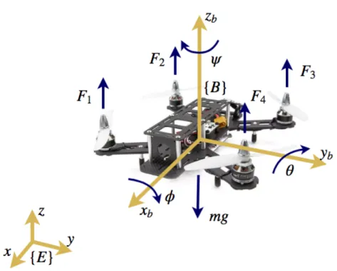
The quad-rotor model is inherently non-linear. The system has four inputs to facil-itate the maneuver in 3-dimensional space. Inertial frame of reference corresponds to the coordinate system with respect to the earth while the body frame of reference corresponds to the coordinate system with respect to vehicle body. Roll, pitch and yaw refers to the rotation of the quad-rotor around x,y and z axis respectively. φ,
θ and ψ denote these angles in the corresponding order. These angles are measured with respect to the body frame. If a quad-rotor starts from rest to a certain point in space, it has to undergo translations and rotations. The rotation matrix RB E
transforms the coordinates from body fixed frame to inertial frame and is given as
RBE = cψcθ−sφsψsθ −cφsψ cψsθ+cθsφsψ cθsψ+cψsφsθ cφcψ sψsθ−cψcθsφ −cφsθ sφ cφcθ , (2.1)
where c(.) and s(.)represent cos and sin functions respectively. In a quad-rotor UAV each rotor generates its own thrust according to the revolution per minute (RPM) of the motor and propeller profile. The following relations relate the thrust and
Chapter 2. System Overview
moment generated by a rotor with its angular velocity.
Fi =kfωi2. (2.2)
Mi =kmωi2, (2.3)
where Fi, Mi and ωi are the thrust, moment and RPM of the ith rotor respectively
and kf and km are the constants depending on the propeller profile.
Four inputs to the system are the total thrust of all four rotors and rolling, pitching and yawing torques.
Figure 2.1: A quadrotor UAV physical model.
Figure 2.1 shows a typical physical model of a quad-rotor UAV. The rolling and pitching torques are generated through the angular momentum and thrust difference between opposite rotors corresponding to each axis. Rotors 1 and 3 are responsible for generating pitching torque and rotors 2 and 4 affect rolling torque. The four
Chapter 2. System Overview
inputs can be written as follows:
u1 = ΣFi, u2 =l(F2−F4),
u3 =l(F1−F3),
u4 =M1−M2+M3−M4,
whereMi is the moment generated by the ith rotor perpendicular to its plane of
rotation.
As stated earlier, a quadrotor is an under-actuated system with four inputs. The conventional inputs to a quadrotor system are
u=hu1 u2 u3 u4
iT
where u1 is the total thrust generated by all four rotors and u2, u3, u4 represent
the rolling, pitching and yawing torques respectively. The states and outputs for the system are given as
xm = h x y z φ θ ψ x˙ y˙ z˙ φ˙ θ˙ ψ˙ iT , ym = h x y z ψ i ,
where x, y and z represent position of the center of quadrotor with respect to the inertial frame of reference {E}whereasφ,θ andψ corresponds to roll, pitch and yaw of the quadrotor body frame with respect to the inertial frame. The model derived from Newton-Euler equations under simplified assumptions ([1]- [2]) can be derived
Chapter 2. System Overview as: ΣFr =ma, (2.4) REB 0 0 u1 − 0 0 mg =m ¨ x ¨ y ¨ z , (2.5) Στr =Iα, (2.6) u2 u3 u4 − p q r ×I p q r =I ˙ p ˙ q ˙ r , (2.7)
wherep,qandrrepresent angular velocities in 3 dimensional body frame of reference {B}. Fr andτr are the three dimensional forces and torques acting on the quadrotor
as a result of thrusts generated by the four rotors. RE
B is the rotation matrix from
body fixed frame to world frame. Z-X-Y convention is considered for this matrix. It is generally useful to express the second set of equations in body frame. Moreover, using the small angle assumption for linear systems the equations in state space form
Chapter 2. System Overview are : ˙ x1 =x7, ˙ x2 =x8, ˙ x3 =x9, ˙ x4 =x10, ˙ x5 =x11, ˙ x6 =x12, ˙
x7 = (cosψsinθ+ cosθsinφsinψ)U1/m,
˙
x8 = (sinψsinθ−cosθsinφcosψ)U1/m,
˙ x9 = (cosφcosθ)U1/m−g, ˙ x10 =x11x12(Iyy−Izz)/Ixx+U2/Ixx, ˙ x11=x10x12(Izz −Ixx)/Iyy+U2/Iyy, ˙ x12 =x10x11(Ixx−Iyy)/Izz+U3/Izz. (2.8)
The nonlinear model given by Equation (2.8) is linearized about the equilibrium point,
x∗m =hx¯ y¯ z¯ 0 0 0 0 0 0 0 0 0
iT
.
where ¯x, ¯y and ¯z are the coordinates in {E} at hover. A general form of linearized system is given by
˙
xm =Axm+Bu,
ym =Cxm+Du,
Chapter 2. System Overview where A= 0 0 0 0 0 0 1 0 0 0 0 0 0 0 0 0 0 0 0 1 0 0 0 0 0 0 0 0 0 0 0 0 1 0 0 0 0 0 0 0 0 0 0 0 0 1 0 0 0 0 0 0 0 0 0 0 0 0 1 0 0 0 0 0 0 0 0 0 0 0 0 1 0 0 0 gx∗6 g gx∗4 0 0 0 0 0 0 0 0 0 −g gx∗6 gx∗5 0 0 0 0 0 0 0 0 0 0 0 0 0 0 0 0 0 0 0 0 0 0 0 0 0 0 0 0 Ixx∗12 Ixx∗11 0 0 0 0 0 0 0 0 0 Iyx∗12 0 Iyx∗10 0 0 0 0 0 0 0 0 0 Izx∗11 Izx∗10 0 , B = 0 0 0 0 0 0 0 0 0 0 0 0 0 0 0 0 0 0 0 0 0 0 0 0 (x∗5+x∗4x∗6)/m 0 0 0 (−x∗4+x6∗x∗5)/m 0 0 0 1/m 0 0 0 0 1/Ixx 0 0 0 0 1/Iyy 0 0 0 0 1/Izz ,
Chapter 2. System Overview C = 1 0 0 0 0 0 0 0 0 0 0 0 0 1 0 0 0 0 0 0 0 0 0 0 0 0 1 0 0 0 0 0 0 0 0 0 0 0 0 0 0 1 0 0 0 0 0 0 , here Ix= Iyy −Izz Ixx , Iy = Izz−Ixx Iyy , Iy = Ixx−Iyy Izz .
2.2
Hardware
Figure 2.2: MARHES Aerial testbed
The MARHES aerial testbed consists of three AscTec Hummingbirds quadrotors flying under vicon motion capture system. The network architecture being used is shown in Figure 2.2. This setup is capable of proving highly accurate feedbacks upto
Chapter 2. System Overview
millimeter accuracy at very fast speeds. However, there was a need for expansion of this aerial testbed especially for robotic swarm and vision based navigation ap-plications. Among the new additions to the testbed includes the new quad fleet of quadrotors based on Luminer QAV250 frames and newly released Intel Aero drones. This new family of quadrotors are equipped with vision capabilities to make them independent of any external feedback sources. This makes them capable of flying inside the motion capture system as well as outside. All the robots are ROS based. This adds a whole set of new possibilities of system modifications. Moreover, it provides more flexibility for a robotics software developer on such kind of systems. Stereo camera is used as a primary vision sensor along-with the IMU to provide VIO in real-time. However, the systems are capable of interfacing more vision sensors such as downward facing monocular cameras for VIO on-board. The new quadrotors have higher payload capacity to accommodate additional sensors. The low -level attitude control system is provided by an open source firmware PX4 on all the sys-tems. Different computers are used for high-level trajectory generation and image processing keeping in view the computational power and efficiency required. Three of those robots are described as follows
2.2.1
LoboDrone
Chapter 2. System Overview
Figure 2.4: Strain and stress measurements.
Figure 2.5: LoboDrone v1.0 quadrotor frame with actuators.
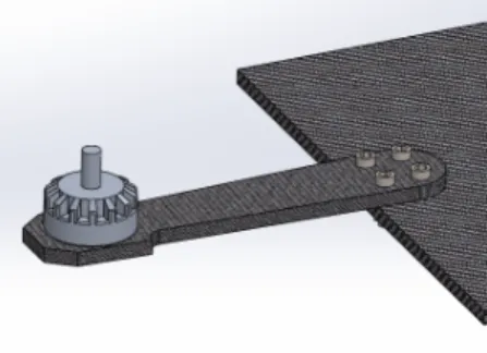
This quadrotor is built from scratch making it fully compatible with the required sensors for perception and planning. The carbon fiber plates are cut to built the frame according to the right size. The case on top carrying the cameras and a USB 3.0 hub is 3D printed. Figure 2.5 shows the picture of the assembled frame without computer and camera.
The frame designed consists of a 4mm carbon fiber bottom plate, on which are bolted four commercially available quadrotor arms. Stand-offs are used to add a second platform, this time made of 2mm carbon fiber. The Jetson is mounted on the bottom plate, and the PixRacer hangs from the top plate. This way, all onboard computing and flight control devices are protected, and the top plate is free to
Chapter 2. System Overview
mount sensors like the ZED camera. The battery is strapped to the bottom of the vehicle. The biggest concern with the custom platform is the joint between the motor arms and the bottom plate, as this joint must carry the weight of the vehicle and remain rigid amidst potentially high forces and torques. SolidWorks is used to run a stress analysis at the joint [42]. To simulate the greatest stress, the bottom plate is fixed and a force is applied to the motor equal to its maximum thrust of 2 kg. The analysis concluded with a maximum possible displacement of 0.103 mm, stress of 1.860e−7N/m2 which we determined, should not pose any issue. Figures 2.3, 2.4, 2.5 show the model of an arm, stress and strain measurements, and physical quadrotor respectively. Pixracer autopilot is used for low-level computational tasks like attitude stabilization with Jetson TK1 for high level trajectory generation and image processing. Both of them are described in the following subsections.
Tiger F80 1900kV motors are used for this platform carrying 6 inch propellers. With this configuration it can carry approximately 100 grams of payload while having a flight time of approximately 3 minutes with a 4s 3300 mAh battery. The airframe itself is 350mm in length when measured from motor shaft to motor shaft diagonally. The weight of this whole platform is approximately 1500 grams including battery and all the electronics.
2.2.2
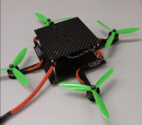
Lumenier QAV250
The newer version of LoboDrone includes a supercomputer with one of the most advanced stereo camera technology on-board. The frame used is Lumenier QAV250 airframe [50]. The airframe weighs 170 grams and is 250mm in length when measured diagonally from motor shaft to motor shaft.
This version is smaller, lighter and has better on-board computer than the first version of LoboDrone. With a 4s 3300mAh battery the flight time is recorded as approximately 10 minutes. The stereo camera used is Zed mini. This is the newest version of Zed camera by Stereo Labs and is designed to be used for mixed-reality
Chapter 2. System Overview
Figure 2.6: LoboDrone v2.0 quadrotor assembly.
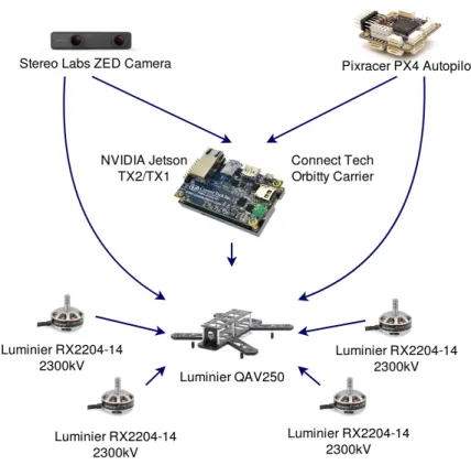
applications. The weight of the whole system including the battery and all the elec-tronics is approximately 900 grams. The actuators used are Lumenier 2204 2300kV motors. The controllers used for these motors are Luminier BL Heli F390 30A electronic speed controllers with autoshot/active braking capability. Oneshot serves as a faster ESC protocol replacing the old pulse width modulation (PWM) proto-col. With 5 inch propellers this setup can carry more payload as well i.e. ≈ 800 grams. Additionally, pixracer flight controller is responsible for performing the low level computational tasks like attitude stabilization while NVIDIA Jetson TX2 is the supercomputer on-board which is used for high level perception and planning computations.
Chapter 2. System Overview
2.2.3
Intel Aero
IntelR Aero flight platform comes as a ready to fly drone kit which is a pre-assembled
quadrotor UAV ready to fly through an RC transmitter. Main sensors and computer boards mounted on this platform are an aero compute board, a flight controller with PX4 autopilot, and an Intel Realsense camera and other required peripherals for flight. Its compute board is an Intel R Atom TM x7-Z8750 processor with 4 GB
LPDDR3-1600 RAM and 32 GB eMMC memory. Attached to it are a forward facing 8MP RGB camera and a downward facing monochrome VGA camera. Moreover, Intel Realsense is well known for its computational capabilities for depth maps. The on-board version of this camera is R200 which is very old now but it can easily be replaced by a newer one. It supports external USB3.0 devices as well. This pre-assembled architecture serves as a good platform for development especially for perception algorithms on-board. Similar to ARM processors, it can run Ubuntu and ROS which can be easily installed on them. Figures 2.7 and 2.13 show the items in an Intel Aero RTF kit and its compute board respectively.
Chapter 2. System Overview
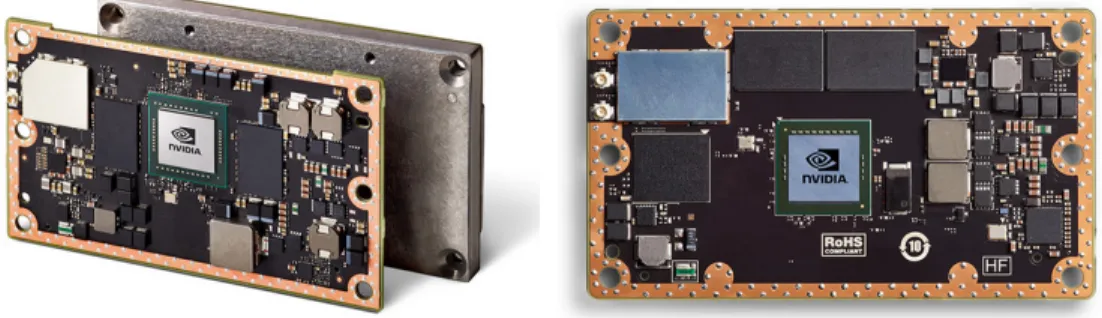
2.2.4
NVIDIA Jetson
NVIDIA took the computational power on robots especially on small autonomous drones to the next level [48]. Jetson TK1 is the first one in the series with NVIDIA 4-Plus-1 TMQuad-Core ARM R CortexTM -A15 CPU and NVIDIA Kepler GPU with
192 CUDA Cores. It has 16 GB internal eMMC memory. Its dimensions are 127mm x 127mm. The newer ones are Jetson TX1 and TX2. They both are supercomputers contained in small modules. Jetson TX1 is the first ever supercomputer on a module. They run on NVIDIA Maxwell TM and Pascal TM GPUs respectively. They both have 256 CUDA Cores and are 50 mm x 87 mm in size which is reasonably small for a small scale quadrotor UAV. CUDA is a programming model and framework for parallel computing. All of them have USB 3.0 and USB 2.0 devices compatibility, 1 Gigabit Ethernet, 802.11ac WLAN and Bluetooth. These features make them very suitable for deep learning, vision and other GPU computing applications on small scale robots. Figures 2.8 and 2.9 show how these modules look like. Jetson TK1 is
Figure 2.8: Jetson TK1.
used in the first prototype of LoboDrone. The main drawback of using it over the other two is that its much larger in size and support Ubuntu 14.04 which does not support the latest softwares like ZED camera SDKs for the newer cameras. Jetson TX1/TX2 has support for Ubuntu 16.04 which solves these problems. Moreover, it can also run ROS Kinetic, the latest stable version of ROS. However, Jetson
Chapter 2. System Overview
Figure 2.9: Jetson TX1 and TX2 modules.
Figure 2.10: Orbitty carrier board on Jetson TX1.
TX1/TX2 cannot be mounted directly on a quadrotor since it does not provide easy interface for the required peripherals. Figure 2.10 shows the orbitty carrier board sold be Connect Tech Inc. It is a 87mm x 50mm lightweight board which provides interface for gigabit ethernet, USB 3.0, USB 2.0, HDMI, MicroSD, 3.3V UART, I2C, and GPIOs. This makes it easier to connect external devices to the Jetson TX1/TX2 modules. This setup is used in the latest revision of LoboDrone using a QAV250 airframe.
Chapter 2. System Overview
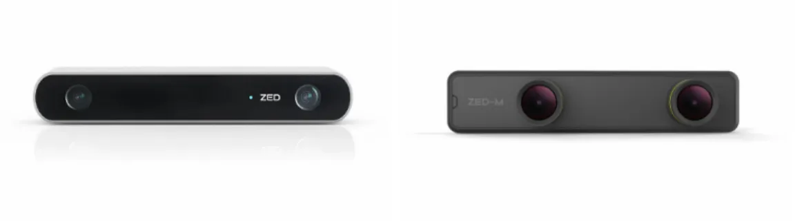
Figure 2.11: ZED and ZED mini stereo cameras.
2.2.5
Stereo Labs ZED Camera
ZED camera being the world’s first 3D camera for motion tracking and depth sensing is the state of the art in stereo vision to facilitate robot navigation [49]. There are two versions of ZED cameras available commercially as shown in Figure 2.11. The older standard ZED camera is a little bigger than the newer ZED mini. Both of them weigh≈160 and≈63 respectively. Both are capable of 6-axis positional tracking and stereo-inertial simultaneous localization and mapping (SLAM). However, the former can compute depth at longer distances i.e. from 0.5 to 20 meters while the later is capable of computing depth from 0.1 to 12 meters. They both have highly accurate motion sensors like accelerometer and gyroscope with sampling rate of 500Hz. They have a position and orientation accuracy of +/−1 mm and 0.1o respectively with
up to 100 Hz refresh rate. The standard ZED can go up to 2K resolution while ZED mini can go up to 2.2K resolution also claiming to be the fastest depth cameras. ZED mini is the first camera for mixed-reality applications. Stereo Labs provides a ROS wrapper to provide an interface for use with ROS. For use with Jetson and ROS on-board, the resolution and refresh rate options become limited accordingly.
Chapter 2. System Overview
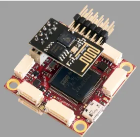
2.2.6
Autopilot PX4
PX4 is an open-source autopilot firmware mainly designed for hobbyist. Using any hardware like pixhawk and its variants, makes it easier to design and test low level control and high level planning algorithms. The main advantage of using such frame-work is that it is compatible with ROS. It accepts commands in the form of ROS topics from any computer running ROS. Since ubuntu and ROS can easily be in-stalled on ARM based processors like Odroid and Jetson, PX4 is very ideally suited as an autopilot for development and other customizations. There are a lot of differ-ent variants of hardware supporting PX4 firmware. One of them is pixracer which is used on both versions of LoboDrones. It has 180 MHz ARM Cortex R M4 with
single-precision FPU and 256 KB SRAM. It has its own WiFi telemetry for getting live data and for firmware upgrades. Moreover, it provides interfaces for the external peripherals needed for flight like PPM input for Spektrum RC receiver, port for FrSky telemetry, and PWM out port for ESCs, SD card slot for logging and safety switch port and other connectors. Most essentially it has the sensors embedded in the mod-ule for flight like barometer, magnetometer/compass, gyroscope and accelerometer. Typically, an on-board computer is used to send trajectories in the form of position set points to the autopilot running PX4 which is assumed to take care of low level attitude stabilization while following the way-points. However, the autopilot-ROS interface, as described in the software section, allows the computer to send low level commands as well if needed. Figure 2.12 shows a pixracer hardware module which can run PX4 autopilot firmware [51]. There are some other platforms which have the autopilot and on-board computer embedded on a single chip. It eliminates the need to buy and mount separate computer and autopilot modules on a robot. Intel Aero is one of the platforms which have such an architecture. It has an intel aero compute board mounted which provides all the computing required for a flight including the PX4 autopilot firmware. Figure 2.13 shows a picture of an Intel aero compute board.
Chapter 2. System Overview
Figure 2.12: A pixracer module
Figure 2.13: An aero compute board.
2.3
Software and Communication
2.3.1
ROS
Robot Operating System (ROS) provides the communication and low level framework for the architecture used. It has a modulated structure where nodes (containing C++ or Python functions) talk to each other using pre-defined classes of packets called ros messages. They can either use publish/subscribe model to route ros messages over user defined topics or use service/client. The former one is ideally suited for many to
Chapter 2. System Overview
many communication while the later is used for request/reply interactions. The whole architecture however, provides support for inter and intra robot node communication. Figure 2.14 shows a simplified version of such a system. Summarizing it, having a lot more to it than just mentioned, ROS is well suited for many robotics applications. It not only provides the communication framework but also software interfaces to many peripherals widely used in robotics. Moreover, its vast open source community adds a lot to the reuse-able software contributions by the developers.
Figure 2.14: Basic ROS concept.
2.3.2
MAVLink Protocol
MAVLink is a communication protocol usually used by the UAVs for the data transfer to and from other devices. PX4 based autopilot modules typically use MAVLink protocol for communication. The wrapper for this protocol for use with ROS is mavros. It converts the MAVLink messages to and from ROS messages on the on-board computer running ROS while the autopilot being connected to any USB port on the computer.
2.3.3
Jetson Setup
As mentioned earlier NVIDIA Jetson is used on most of the vision equipped robots at the MARHES testbed. These Jetson board accompany JetPack which is a software that is used to flash the board with customized versions of Linux, opencv, CUDA
Chapter 2. System Overview
toolkit and many other vision and deep learning software libraries. Its latest release is JetPack 3.2 which comes with Linux for Tegra (L4T) 28.2, which is a lighter Ubuntu 16.04 adapted to use with Jetson TX1, TX2/TX2i. It also comes with CUDA 9.0 which is required by ZED mini software development kit (SDK) and ROS-wrapper. It requires a host PC running Ubuntu 14.04 or 16.04 to flash the board. Once the JetPack installation is complete, ROS and can easily be installed and its packages can be developed. Similar procedure can be used to setup TK1 but it only supports the outdated versions of these softwares which makes the development more difficult.
2.3.4
ZED Camera Setup
A ZED camera comes with its own SDK for developers. However, by using ros-wrapper for a particular SDK, the development environment can be changed to ROS which provides necessary messages and topics to subscribe from and publish to. The latest version of ZED SDK is 2.4 which is supported by Jetson TX1 and TX2. It works with JetPack 3.2 and CUDA 9.0. As mentioned earlier when SDK is used with ROS-wrapper it publishes the odometry, the coordinate frames transformations, the rectified and raw image topics for all the cameras and depth and the point cloud in the form of ROS messages.
Chapter 3
Perception
3.1
Stereo Camera Model
Stereo camera is used to compute depth of the scene. A stereo camera takes ad-vantage of two cameras to calculate the disparity through triangulation. This is governed by epipolar geometry.
3.1.1
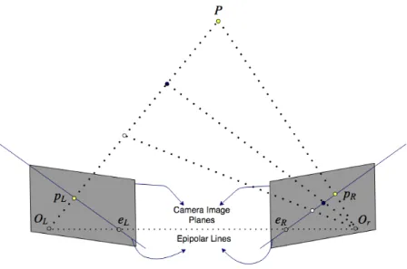
Epipolar Geometry
Epipolar geometry can be visualized in Figures 3.1 and 3.2. Figure 3.1 shows two camera planes at some angle. OL and OR represent the optical centers of the two
cameras. An optical center is a point from where all the projection lines of a camera must pass. This is also known as camera center. Stereo vision set up includes two epipoles, one for each camera. They are labeled as eL and eR respectively. The
epipole eL refers to the point where the projection line from the optical center of
the right camera intersects the image plane of right camera. In other words it is the image of the right camera’s optical center as seen by the left camera. The opposite applies to the epipole eR. Consider a point P in space. The line joining the optical
Chapter 3. Perception
Figure 3.1: Epipolar geometry with non-parallel camera frames.
Figure 3.2: Epipolar geometry with parallel camera planes.
plane. The projection of this line in the right image plane is known as epipolar line. The pointP and bothOLandORlie in one plane called epipolar plane. The epipolar
Chapter 3. Perception
Any point projected in the left image plane can be the projection of one of the points on lineP OL, in the right image plane. Therefore, the pointpLmust appear on
the epipolar line pReR. This is called epipolar constraint. Once that point is found
depth is calculated through triangulation. In case of cameras with parallel image planes, the epipolar line will become a horizontal line as shown in Figure 3.2 and the point pL can be found by matching it with the pixels on this line.
3.1.2
Pinhole Camera Model and Triangulation
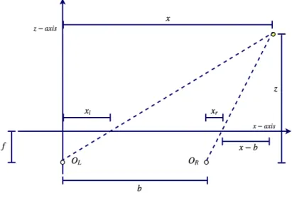
Figure 3.3: Triangulation geometry.
A pinhole camera model for both the cameras can be used to calculate the depth from disparity by a process called triangulation. Let f be the focal length of the camera. It is defined as the distance from the optical center of a camera to its image plane. bis the stereo baseline which refers to the distance between two optical centers. The stereo vision setup is shown in Figure 3.3. If we know the pixel values of the projection of point P we know the projection lines and hence we can utilize
Chapter 3. Perception
some principles from geometry. From similar triangles,
z f = x xl, z f = x−b xr , z f = y yr = y yl.
The depth can be calculated from triangulation:
z =f×b/(xl−xr) = f×b/d, x=xl×z/f = (b+xr)×z/f, y=yl×z/f =yr×z/f.
It can be noted that the disparity d is inversely proportional to depth of a pixel. A pinhole camera model is considered for depth space collision checking.
3.1.3
Calibration Parameters
The calibration of a stereo camera yields two set of parameters for each of the two cameras. They are known as intrinsic and extrinsic parameters. The former refers to the parameters such as focal length, the location of the optical center in an image (in pixels) while the later contains parameters such as relative rotation and translation between the two cameras. Since the camera is modeled based on pinhole model, the conversion from homogeneous camera to homogeneous image coordinates is governed by the following projection equations:
r ∼ICP = f sx 0 cx 0 0 f sy cy 0 0 0 1 0 x y z 1 .
If we want to write the projection equations from the homogeneous robot to homo-geneous image coordinates we have to include the rotation and translation of the camera frame with respect to the robot frame and ultimately the world (or inertial frame). The camera frame is attached to the robot frame and all the computations
Chapter 3. Perception
are done in the world coordinates. The above equation can be written as [12]:
r ∼ f sx 0 cx 0 0 f sy cy 0 0 0 1 0 RCI T 0 1 x y z 1 . (3.1)
Here r is the pixel coordinate corresponding to point P. sx and sy are the pixel
dimensions and cx and cy are the image frame coordinates of the location of camera
optical axis.
3.2
Perception Strategy
Figure 3.4: Computation of the artificial shields and their transformations and pro-jections in the depth image space.
While solving for path planning and collision avoidance problems in real-time, the need for an algorithm for efficient collision checking is inevitable. One way to do this is to make a 3-D occupancy grid and update it continuously in real-time using local vision data. However, this requires slightly more computation than necessary. A lot of work has been done using this idea of mapping the local subsets of the
Chapter 3. Perception
whole configuration space. However, by performing the collision checking directly in depth-image space proved to be much faster. It is also more effective in the presence of image noise. This can also be called planning in perception space. The perception problem can be formulated as following.
Let the discrete trajectory generated by the controller to be qs(x0, li, n) ⊂ C
where x0 is the initial state, li is the current mode and 0 < n < (Th +Tsaf ety)/Ts
is the local time of the generated potential trajectory. This trajectory has to be checked for collision before appending it in the final set of desired trajectories qd(k).
Here k is the global trajectory time since the start of the system. For simplicity the potential patch of the trajectory to be checked for collision and the final desired trajectory will be referred to as qn
s and qdk respectively. The perception problem
is to find the function P : C → CState where CState = {0,1,2} represents the collision state of the configuration. 0 and 1 collision states mean thatqn
s ∈ Cf ree and
qsn∈ Cobs respectively, while 2 means that the configuration is out of the field of view
at a particular time when the check is performed i.e. qn
s ∈ G/ (q(kc)). Here q(kc) is
the current configuration of the quadrotor when the check is performed.
The collision detection is performed purely in depth space by exploiting the pro-jection equations and the stereo camera model as described above. The motion planner generates a discrete trajectory in the form of set of points through the con-figuration space. Given a point in the concon-figuration space, it can be checked whether it is in collision by projecting the robot in depth space. The quadrotor projection in depth space can be simplified as a projection of set of all points contained in a square. This square can be considered as a ’shield’ for a quadrotor. The size of this square is assumed to be slightly larger than the longest dimension of the quadrotor while its position is such that its placed at some distance ψx in front of the the quadrotor
inFW. This is a pessimistic version of the strategy presented in [12] which considers
the projections of the surface normals of a quadrotor as a shield. This shield keeps on changing shape depending on the configuration. However, we considered the
con-Chapter 3. Perception
stant size of this square corresponding to the maximum size as of that proposed by the above reference.
The idea is that given a query pointqn
s in FW, a corresponding artificial square
shield is generated (Figure 3.4). This square refers to the set s(qsn) = {q :qsn(1)−
ψy <q(1) <qsn(1)+ψy & qns(2)−ψz <q(2)<qns(2)+ψz & q(0) =qsn(0)+ψx},
where ψx, ψy and ψz are the safety margins in corresponding directions. After the
computation of set s(qsn) for the query point qsn, all the points contained in the set are first transformed in the vehicle body coordinate system and ultimately the camera coordinate system depending on the current quadrotor pose at time instant
kc and the pose of the attached stereo camera with respect to the vehicle body. This
transformation is followed by a projection of s(qn
s) on the depth image. Combining
these expressions we get Equation (3.1). Here RC
I refers to the rotation from world
(or inertial) frame to camera coordinate frame.
RCI =RCB×RBI. (3.2)
where RC
B = Ry(−π/2)× Rx(π/2) is the rotation matrix from body to camera
coordinate system and RBI is the ZXY rotation matrix corresponding to the current orientation of the robot.
The query trajectory point qn
s is assumed to be collision free if all the points
contained in the corresponding set s(qn
s) are collision free. It is outside the field of
view if any point on the set does not correspond to a valid image point. Similarly, it is in collision if any point in that set is under collision. Given any point C ⊃ q = (x, y, z, θ) in world frame, it is transformed to a corresponding point C ⊃qT =
(xT, yT, zT, θ) in camera coordinates and projected to pixelr on the depth image. xT yT zT 1 = RCI T 0 1 x y z 1 .
Chapter 3. Perception
Formally,
P(q) = 0 if D(r)> zT ∀q∈s(qsn), P(q) = 1 otherwise,
It can be noted here that rotation in place (θ) for the query trajectory points will not affect the collision detection because the quadrotor geometry is approximated by a rectangular ’shield’ with safety margins in FW. Function D(r) refers to the depth
of a pixel r.
3.3
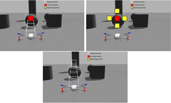
Escape Strategy
Figure 3.5: Escape point computation by querying potential points in 4 directions.
In the eventP(qns) = 1, i.e. if the predicted trajectory experiences collision, the vehicle has to be deviated to the safe location. This location is referred to as escape point, the corresponding configuration and state vector is qesc and xesc respectively,
Chapter 3. Perception
consideringθand the final velocities as 0. Let any trajectory pointqns be in potential collision, the image space in the neighborhood of this point iny−z plane is searched for the high depth areas. Since searching the whole depth image in a continuous way is computationally expensive and time consuming, the search is performed in 4 different directions with discrete intervals. This quadrotor is projected in the depth space some distance dl away from qsn in up, down, left and right directions and
checked for collisions. This process is repeated with more projections at distance dl
from previously checked points, until a collision free point is found. This point is the escape point. To prevent the planner from getting stuck at a place in case of another obstacle suddenly appearing after the first one, the projections are performed in an
y−z plane a little way from the plane associated with qn
s. Figure 3.5 shows how the
Chapter 4
Control Strategy
4.1
Trajectory Generation
The trajectory generation is performed in 3-D, utilizing a pre-computed set of control laws. While the first feedback law ua tries to take the system to a global goal, the
other feedback law ub is responsible to divert the system from possible collisions.
The state vector in continuous time can be written as,
x=hx x y˙ y z˙ z˙
iT
.
It is assumed that the vehicle’s frame always coincide with FW and a low level
controller takes care of maintaining the heading. A double integrator model is used where: ¨ x=u1, (4.1) ¨ y=u2, (4.2) ¨ z =u3. (4.3)
The differential equations are discretized with a sampling time ofTsto obtain discrete
system matrices.
x(k+ 1) =Adx(k) +Bdu(k), (4.4)
Chapter 4. Control Strategy
The two control laws are given as,
ua =Kax, (4.6)
ub =Kbx. (4.7)
Trajectories are generated in a receding horizon way with the time horizon of Th.
In order to ensure real-time flight speeds the trajectory planning and execution are performed in parallel using multi-threading in Robot Operating System (ROS). First thread subscribes to the depth image data whenever it arrives, queries the next patch of trajectory from the controller according to the current mode, checks each point in the trajectory for collisions, and appends the valid or an empty trajectory at the end of desired trajectory qk
d. Each patch qns appended is of time Th. While this thread
keeps on appending the trajectories irrespective of where the vehicle is, the other thread keeps sending the way-points from the trajectory qdk after every Ts. While
querying a potential patch of trajectory qn
s for collision, if any point is in collision
the trajectory is discarded and the system enters the obstacle-avoid mode, while in case of a collision free predicted trajectory it is kept. However, if any point is out of the field of view its simply discarded without any mode change so the planner can keep on querying, in a hope that the trajectory will get into the field of view while the quadrotor maneuvers result in changes of position and orientation of the attached camera.
To improve functionality of the algorithm the potential patch of trajectory sent by the controller is slightly longer than time Th. This is done to ensure that the
collision-free trajectory being appended does not take the quadrotor very close to any obstacle from where getting out becomes impossible under camera’s field of view and other vehicle dynamics limitations. This trajectory is therefore generated for
Th+Tsaf ety and queried for collisions. In case of no collisions the first half of the
trajectory for time Th is kept and appended. This ensures that while the vehicle
maintains a particular mode the collision is detected and planned to be avoided before Th to Tsaf ety seconds. Here Tsaf ety is the the safety time and is set smaller
Chapter 4. Control Strategy
than the time horizon Th.
4.2
Hybrid System Perspective
Figure 4.1: Hybrid automaton.
The hybrid automatonH is a collectionH = (L,X,Init,f, Inv,E, G, R) [30], where
1. L is a set of discrete variables (or modes)
Chapter 4. Control Strategy
3. Init⊆L×X is a set of initial states
4. f ={f1, f2, f3} is a set of vector fields or systems dynamics for each l∈L
5. Inv assigns to each l∈L an invariant seti.e. Inv(l)⊂x
6. E is the collection of discrete transitions
7. G assigns to each e= (l, l0)∈E a guard
8. R assigns to eache= (l, l0)∈E and x∈X a reset condition
The system undergoes two different types of manuevers defined by the motion prim-itives at each state x(k) depending on the current discrete mode lk. [31] Let the
allowed motion primitives for any statex(k) be a setUp(x(k)) ={u
a,ub}. For each
sampling time interval (i.e. fromx(k) to x(k+ 1)) the system experiences an input
u∈ Up related to the state x(k) by Equation 4.6. The hybrid automaton comprises
of 2 modes.
Mode 0
Mode 0 (l0) is responsible for taking the quad-rotor to the goal position with an
objective to minimize the state error as well as the energy. In other words, the controller for this mode is defined as:
ua ={u :minu X
Chapter 4. Control Strategy where Q= 1 0 0 0 0 0 0 0.1 0 0 0 0 0 0 1 0 0 0 0 0 0 0.1 0 0 0 0 0 0 1 0 0 0 0 0 0 0.1 , R= 3 0 0 0 3 0 0 0 3 .
Two of the guard associated with this mode areG(l0, l1),G(l0, l2). G(l0, l1) is enabled
when a collision is detected in trajectory qn
s for any 0 < n < (Th +Tsaf ety)/Ts i.e.
the collision in some future time becomes inevitable if the quadrotor stays in this mode. G(l0, l2) is enabled when the quadrotor reaches goal configuration qgoal at 0
velocity in all three dimensions as mentioned in Section 1.4. This final goal state
xgoal corresponds to the qgoal given the velocities in three dimensions. Therefore,
there is an easy mapping between a state x and the configuration at that state q. Hence, the objective of controller in this mode is to take the quadrotor to its destination y −z plane with zero final velocity while minimizing the energy/fuel consumption. However, in case of an obstacle on the way, the system goes to mode 2 where the objective is primarily to deviate quickly without caring much about the energy minimization.
Mode 1
Mode 1 (l1) is responsible for taking the quad-rotor to the temporary escape
config-uration with an objective to minimize more the state error rather than the energy. In other words, the controller for this mode is defined as:
ub ={u:minu X
Chapter 4. Control Strategy where Q= 1 0 0 0 0 0 0 0.1 0 0 0 0 0 0 1 0 0 0 0 0 0 0.1 0 0 0 0 0 0 1 0 0 0 0 0 0 0.1 , R= 0.1 0 0 0 0.1 0 0 0 0.1 .
Two of the guard associated with this mode are G(l0, l1), G(l1, l0). G(l0, l1) is
ex-plained in the above section. G(l1, l0) is enabled when the quadrotor reaches escape
configuration qesc at 0 velocity in all three dimensions. The perception algorithm
makes sure that before switching to this mode from mode 0, it performs the check in four predefined directions from the predicted collision point and tries to find a collision free point in 3D that is closest to the collision point in y−z plane corre-sponding to the collision point. The given 3D point corresponds to the configuration in C because θ is assumed to be 0. This configuration can be easily converted to state vector x by appending 0s for the velocity terms.
Hence, the objective of controller in this mode is to take the quadrotor to an escape point with zero final velocity to have a clearer view of what is beyond the obstacle. Less weights on the energy is inspired from the fact that in case of a sudden interruption in vechicle’s way, it must take measures to quickly maneuver away to a point from where it can potentially see its destination clearly.
Chapter 4. Control Strategy
4.3
Proof of Hybrid System’s Stability
Since the trajectory generation follows either of the two pre-computed LQR feedback laws, the concern of system’s stability while mode switching is of great importance. As mentioned before the first feedback lawuatries to take the system to a global goal
while the second feedback law ub takes the system to a temporary escape point as
mentioned in Equations 4.6. Two different controls objectives leads to two Lyapunov functions. Figures 4.2 and 4.3 show these set of Lyapunov functions for a particular case. Here xref and xesc are the equilibrium points of first and second Lyapunov
functions respectively.
An interesting fact about combining real-time perception and hybrid control the-ory is that even though the first Lyapunov function remains the same for the whole maneuver, the second Lyapunov function changes its location i.e. it slides relative to the first Lyapunov function based on where the obstacle is encountered. Every time the obstacle is encountered at a different location the overlapping regions of the two Lyapunov functions change. Therefore, we will prove that under certain assumptions on the regions in Lyapunov functions the switching is always stable. These assumptions include that the obstacle is always closer than the global goal and that the switching occurs before the quadrotor reaches obstacle location. For instance, in a particular case of Figure 4.3, Ri
e, i∈ {1,2}refers to the region where
the system cannot enter practically while staying in the corresponding mode. Since the obstacle is located at 4m, the system is assumed to enter mode 1, before entering region R2e.
Lets take the second order subsystem forx dimension,
x= [x(k) x(k+ 1)]T.
The corresponding Lyapunov functions for each control law are given as:
V1(x) = (x−xref)TP1(x−xref), (4.8) V2(x) = (x−xesc)TP2(x−xesc). (4.9)
Chapter 4. Control Strategy
Figure 4.2: Lyapunov function For xref = [10 0] and xesc = [4 0].
Figure 4.3: Lyapunov function (Zoomed-In) For xref = [10 0] and xesc = [4 0].
Herexref ∈xand xesc ∈xare the global reference state and the obstacle state inx
Chapter 4. Control Strategy
discrete time systems:
ATPiA−Pi+Q= 0 i∈0,1. (4.10)
According to Rayleigh-Ritz inequality for symmetric matrices,
λ1(min)||x−xref|| ≤V1(x)≤λ1(max)||x−xref||, (4.11) λ2(min)||x−xesc|| ≤V2(x)≤λ2(max)||x−xesc||. (4.12)
The system is undergoing stable switching if ([47])
V1(xs)−V2(xs)>0, (4.13)
or
λ1||xs−xref|| −λ2||xs−xesc||>0, (4.14)
where xs is any state at which switching occurs [29] [30]. The domain Ds :R2 →R2
of x where the switching is possible to occur is given as:
Ds(x) ={x|x(0)<xesc(0)<xref(0)}. (4.15)
It can be noted that our system has repeated eigen values for both modes, i.e.
λ1(min) = λ1(max) = λ1 = 3.3781 and λ2(min) = λ2(max) = λ2 = 1.6640. We have to
find out that within our domain of xs, whether the switching is stable. Expanding
Equation 4.14,
(λ1−λ2)||xs||+λ1||xref|| −λ2||xesc||
−2λ1(xs(0)xref(0) +xs(1)xref(1))
+2λ2(xs(0)xesc(0) +xs(1)xesc(1)) >0.
Since the two optimas have zero velocity, we can put them equal to zero, (λ1−λ2)||xs||+λ1xref(0)2−λ2xesc(0)2
−2λ1xs(0)xref(0) + 2λ2xs(0)xesc(0)>0.
Adding and subtracting λ1xs(0)2−λ2xs(0)2 on both sides:
(λ1−λ2)||xs||+λ1(xref(0)2−2xs(0)xref(0) +xs(0)2)
−λ2(xesc(0)2−2xs(0)xesc(0) +xs(0)2)
Chapter 4. Control Strategy
Simplifying further leads to:
(λ1−λ2)xs(1)2+λ1(xref(0)−xs(0))2−λ2(xesc(0)−xs(0))2 >0.
It should be noted that λ1 > λ2. Consequently, the first term is always greater
than 0. The second and the third terms are also always greater than 0 if xref(0) >
xesc(0) > xs(0) (i.e. if xs ∈ Ds(x)). Therefore, the hybrid system’s stability is
Chapter 5
Verification and Applications
5.1
Tracking Results
The experiments could not be performed in the VICON testbed because of the scale of these experiments. Exploiting the system’s capabilities of computing visual-inertial odometry (VIO) from the on-board sensors provides a viable solution. We are using a single forward-facing camera for all vision related tasks. Before moving further with the experiments, the trajectory tracking capabilities have to be evaluated. This is done based on its performance to track a figure eight trajectory which can be a difficult trajectory to track if the system is unstable. The system is first evaluated in the motion capture system before moving on to using VIO. The trajectory is generated utilizing the concept of the lissajous figures. Combination of sine waves are used to compute the figure eight trajectory. Figure 5.1 (left) shows the results of figure eight trajectory tracking inside the VICON motion capture system. The performance seems better in this setup for obvious reasons but ZED camera brings the state-of-the-art stereo SLAM technology which makes the trajectory tracking stable even though the camera is mounted in the forward facing manner which seems quite reasonable. Figure 5.1 (right) shows the trajectory tracking in on-board vision setup.