Predicting Supply Chain Risks Using Machine
Learning: The Trade-off Between Performance and
Interpretability
George Baryannisa, Samir Danib, Grigoris Antonioua aDepartment of Computer Science, University of Huddersfield, UK
bDepartment of Logistics, Marketing, Hospitality and Analytics, University of Huddersfield,
UK
Abstract
Managing supply chain risks has received increased attention in recent years, aiming to shield supply chains from disruptions by predicting their occurrence and mitigating their adverse effects. At the same time, the resurgence of Artifi-cial Intelligence (AI) has led to the investigation of machine learning techniques and their applicability in supply chain risk management. However, most works focus on prediction performance and neglect the importance of interpretability so that results can be understood by supply chain practitioners, helping them make decisions that can mitigate or prevent risks from occurring. In this work, we first propose a supply chain risk prediction framework using data-driven AI techniques and relying on the synergy between AI and supply chain experts. We then explore the trade-off between prediction performance and interpretability by implementing and applying the framework on the case of predicting deliv-ery delays in a real-world multi-tier manufacturing supply chain. Experiment results show that prioritising interpretability over performance may require a level of compromise, especially with regard to average precision scores.
Keywords: supply chain risk management, risk analysis, risk prediction, machine learning, interpretability
∗Corresponding author
1. Introduction
Managing risks in supply chains at a local, national, or global scale has increasingly attracted attention from both researchers and practitioners in re-cent years, owing in part to the worldwide economic uncertainty that began with the 2008 global financial crisis. The field of supply chain risk manage-5
ment (SCRM), which emerged in the early 2000s has now become more than the overlap of directly related areas such as enterprise risk management and supply chain management [1]. As defined in [2], SCRM “encompasses the col-laborative and coordinated efforts of all parties involved in a supply chain to identify, assess, mitigate and monitor risks with the aim to reduce vulnerability 10
and increase robustness and resilience of the supply chain, ensuring profitability and continuity”.
The wide range of decisions and actions that are involved in SCRM have led to an equally wide spectrum of solutions proposed by researchers. These can be broadly classified in three categories: (1) multiple-criteria decision anal-15
ysis techniques; (2) mathematical modelling and optimisation; and (3) Artificial Intelligence (AI) techniques. The first category includes well-established tech-niques to evaluate different risk-related criteria that affect supply chains, as well as the efficiency of potential solutions, such as analytic hierarchy process [3] or data envelopment analysis [4]. The second category is by far the most common 20
one (as analysed in [2, 5]) and includes approached based on stochastic or fuzzy programming and robust optimisation.
AI techniques have received relatively little attention in relation to SCRM or supply chain research, in general. Recently, there has been an AI resurgence due to the availability of increased computing power and large amounts of data, 25
as well as the success of approaches within the broad area of machine learning. This has also led to SCRM researchers considering the potential of AI tech-niques in relation to tasks such as risk identification, prediction, assessment and response [6, 7, 8, 9]. However, research is still at early stages, proposing either purely theoretical frameworks that have not been implemented and applied in 30
real-world case studies [6, 7], or ad-hoc solutions that are only applicable within the confines of a particular case study [8, 9]. Also, these works do not take into account the data imbalance which is inherent in risk-related tasks, since for many risks the ratio of occurrence and non-occurrence is far from balanced.
More importantly, research that uses data-driven AI for SCRM does not 35
take into account the importance of interpretability of results: no conclusions are derived in relation to the reasons behind the results of the machine learning models they create. As stated by Doshi-Velez and Kim [10], most real-world tasks addressed using machine learning techniques cannot be described merely through a result of a single metric, such as classification accuracy. Similarly, 40
Domingos [11] posits that instead of accuracy and computational cost, learners should be evaluated based on how much human effort is saved or how much insight is gained. Some of the reasons cited by Molnar [12] in support of in-terpretability are directly relevant to SCRM: (1) finding meaning withing and gaining the knowledge captured by machine learning models; (2) detecting bias 45
in models; and (3) increase acceptance of produced solutions. In the context of supply chains, we argue that in order for any results coming out of AI solu-tions to be useful and able to be integrated in SCRM-related decision-making processes, they have to be interpretable and justifiable.
The research hypothesis investigated in this article is the possibility of utilis-50
ing machine learning technologies to provide predictive analytics for SCRM that deliver results that are simultaneously interpretable and of a high prediction per-formance standard. In that sense, we aim to contribute to research in exploring the untapped potential of data-driven AI techniques within SCRM, as identified in [2]. We address the aforementioned limitations by focusing on the particular 55
task of predicting supply chain risks and propose a generic data-driven risk pre-diction framework that takes into account the special characteristics of SCRM. The proposed framework is then implemented and applied on a real-world case study, investigating a variety of metrics and two well-known machine learn-ing algorithms, one less and one highly interpretable: support vector machines 60
is achieved through classification. Classifiers are trained to determine whether a delivery is late or not and are then used on unseen data to predict whether future deliveries will be late or not, in other words whether there is a risk of delayed delivery or not. The novelty of the presented research lies not in the 65
employed algorithms which are well-established and whose choice is indicative, but rather in the manner in which such technologies are to be integrated in an SCRM process. Specifically, the contributions of this article are the following:
• A data-driven risk prediction framework that places emphasis on the syn-ergy between AI and supply chain experts, especially with regard to the 70
proper selection of suitable metrics and algorithms according to the goals and priorities of the supply chain. The proposed framework also takes into account imbalanced data, a common occurrence in risk prediction.
• An implementation of the proposed framework that demonstrates the framework’s applicability in predicting delays in deliveries within a real-75
world multi-tier aerospace manufacturing supply chain.
• Quantification of the trade-off between interpretability and prediction per-formance through experiments for the particular case study.
The remainder of this article is organized as follows. Section 2 offers a concise summary of research efforts that apply data-driven AI techniques for 80
SCRM-related purposes. Section 3 introduces our data-driven risk prediction framework and analyses the individual phases within from both AI and SCRM perspectives. Section 4 illustrates the applicability for SCRM within a real-world supply chain. Then, Section 5 presents results of using the implemented framework to predict delays in deliveries within the studied supply chain. These 85
results are discussed in Section 6, with an emphasis on the trade-off between per-formance and interpretability, as well as the importance of feature-rich datasets and the effect of imbalanced datasets. Finally, Section 7 concludes and proposes directions for future research at the confluence of AI and SCRM.
2. Related Work 90
The potential of applying big data analytics and machine learning techniques for SCRM has recently been considered in literature. Fan et al. [6] investigate potential big data sources related to supply chains and then propose an SCRM framework that relies on the availability of such data. The framework relies on analysing and monitoring supply chain data to detect emerging risks, maintain 95
relevant risk reports and use these to initiate suitable actions such as replanning the supply chain. He et al. [7] similarly acknowledge the predictive capabilities of big data analytics and incorporate such a component within a generic SCRM process model. However, both of these works are purely theoretical in nature, without implementing or applying the proposed frameworks and models to a 100
real-world case study.
To the best of our knowledge, only three articles in literature have applied big data analytics and machine learning techniques for the purposes of risk identification through detection or prediction within an SCRM process and, hence, are directly relevant to the purposes of this work. These are analysed in 105
Section 2.1. There is also a number of additional articles that are less relevant, in that they investigate similar techniques but for different facets of SCRM, specifically assessing and responding to risks. These are the focus of Section 2.2.
2.1. Risk Identification
Zage et al. [8] address supply chain security risks by proposing methods for 110
identifying deceptive practices within the supply chain, specifically for the e-commerce domain. The approach relies on spectral analysis to analyse large amounts of online transactions to determine traces of the so-called fraudster-accomplice strategy: fraudulent vendors interacting exclusively with real or fake users with good reputation to indirectly and artificially build their a good rep-115
utation for themselves. This process leads to developing graph-based metrics which are used by semi-supervised clustering algorithms to accurately determine whether a vendor behaves similarly to a fraudster, based on minimal labeled data.
Ye et al. [9] investigate the applicability of machine learning techniques to 120
identify supply chain disruptions that are rooted in the economic performance of firms within the chain. Publically available financial data, such as asset-liability ratio, are obtained for Chinese firms and for periods before, during and after some form of supply chain disruption took place. Part of these data are used to determine classes of similar firms in terms of financial performance. 125
The rest are used as features in a multi-class SVM classifier, to determine links between financial performance and disruption. The resulting system is capable of determining whether a particular firm exhibits a similar financial profile to ones that have contributed to disruptions in the past.
Both of the aforementioned works [8, 9] present ad-hoc solutions specifically 130
aimed at the particular case studies they focus on. Also, their choice of algo-rithms and metrics does not take into account interpretability or imbalanced datasets. In contrast, our work proposes a generic framework for predicting risks using data-driven AI, which can be applicable to any SCRM-related effort and which places great emphasis on making the right choice of which algorithm 135
and metric to use, based on the supply chain’s goals and priorities and the characteristics of available data.
The case of increasing supply chain sustainability through risk mitigation is explored in Mani et al. [13]. In particular, they use data collected through an Internet-of-Things software platform for fleet management and vehicle tracking. 140
Data involves distances travelled, fleet utilisation, vehicle speeds and stoppages and geo-fencing reports. The authors propose several risk-related usages of such data, such as: (1) identifying underutilised vehicles and optimise fleet to reduce carbon footprint; (2) identifying cases of vehicle seizure by law enforcement through geo-fencing data; and (3) using vehicle stoppage data to identify theft 145
and unethical behaviour. However, the focus is on the use of statistical analy-sis methods, rather than providing some form of predictive capability through learning. Also, while the authors go into great detail about the relevant data, there is no discussion with regard to the implementation and evaluation of the analytics algorithms they employ.
2.2. Risk Assessment and Response
Machine learning and big data analytics have also been used in relation to risk assessment. The earliest attempt to incorporate machine learning tech-niques within SCRM is the use of Artificial Neural Networks (ANNs) by Bruz-zone and Orsoni [14] to assess production losses. The ANNs are trained in a 155
supervised mode, supplying them with specific scenarios correlating production times, quantities and capacities with corresponding cost estimates. Based on these training data, the ANNs learn how to correlate production characteristics with actual gains or losses, in order to then be able to assess and calculate cost estimates for scenarios with an unknown outcome.
160
Bayesian networks have shown great potential in modeling for risk assess-ment, especially in the area of safety risk analysis [15, 16]. Two groups of researchers have identified this potential in relation to a specific aspect of the supply chain risk assessment process, namely risk propagation. Garvey et al. [17] use Bayesian networks to model risk dependency graphs which have the ability 165
to adapt when new knowledge is acquired, thus making sure that risk propaga-tion is modelled accurately. Ojha et al. [18] perform a similar analysis of risk propagation using Bayesian networks, automatically learning the interconnec-tions between several risk factors for different supply chain stakeholders and using this knowledge to determine probability of occurrence and cost for risks. 170
Instead of a (parametric) Bayesian network, Shang et al. [19] introduce a non-parametric Bayes model to assess transport time risks in air cargo supply chains. The authors show how the model can be used as the foundation for several data-driven strategic decisions, such as ranking suppliers at the route level, or higher. A number of studies employ big data analytics in relation to risk response. 175
Papadopoulos et al. [20] employ a data-driven approach to determine factors enabling supply chain resilience, highlighting the importance of swift trust and quality information sharing. Li and Wang [21], on the other hand, use sensor-based data within a food supply chain to dynamically predict the product time-temperature profile; this enables firms to adjust their pricing schemes accord-180
recognise the effect of incomplete or imperfect knowledge in managing disrup-tion risks and propose a Bayesian learning model to increase robustness in the evaluation of inventory and sourcing strategies of a manufacturer in response to risks. Finally, Zhao and Yu [23] explore the potential of machine learning in the 185
context of supplier selection. Their work relies on data from several past cases of selecting suppliers which are clustered based on similarity and are subsequently fed into a back-propagation ANN to extract rules for optimal supplier selection. While not directly comparable to our work, the studies summarised in this subsection show the applicability and potential benefits of machine learning 190
and data-driven approaches on a wide array of issues throughout the SCRM process. In general, even though such techniques represent only a small minority of SCRM research (e.g. compared to mathematical programming techniques, as discussed in [2]), their integration in standard SCRM processes can prove advantageous, as evidenced by the results within the studies presented in this 195
section.
3. Data-Driven Risk Prediction Framework
To enhance supply chain risk prediction, we propose a framework that relies on the integration of artificial intelligence within the SCRM process. The frame-work aims for a two-way interactivity and synergy between supply chain and AI 200
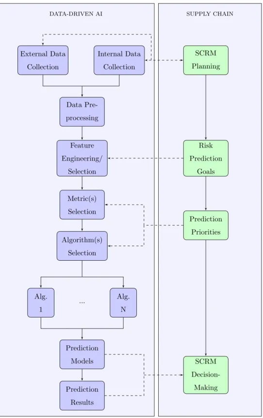
experts: any decision by the AI experts depends on specific input by the supply chain, while any models and results produced have to be interpretable so that they can influence SCRM decision-making. Figure 1 illustrates the framework’s process flow. On the right-hand side of the figure, the focus is on traditional tasks included in a standard SCRM process. The left-hand side includes the 205
major tasks that are involved in a data-driven AI methodology. As should be obvious, the framework relies on effective synergies between a team involved in managing risks within a supply chain and a team specialising in data-driven AI. The remainder of this section is devoted to an in-depth analysis of the proposed framework.
DATA-DRIVEN AI SUPPLY CHAIN External Data Collection Internal Data Collection SCRM Planning Data Pre-processing Feature Engineering/ Selection Risk Prediction Goals Metric(s) Selection Algorithm(s) Selection Prediction Priorities Alg. 1 Alg. N ... Prediction Models Prediction Results SCRM Decision-Making
3.1. Planning and Data Collection
The effectiveness of the proposed risk prediction framework relies on two fundamental prerequisite characteristics. First, a risk management plan needs to be created for the supply chain at hand. This plan should clarify the objec-tives and define the scope of risk management. Indicative questions that would 215
need addressing in terms of objectives include why SCRM is necessary, what outcome is needed and when and which decisions are required and when. In terms of scope, relevant parties should decide whether the focus is the focal firm, risks internal or external to the SC and the specific types of these risks (e.g. environmental, supply, demand, process or control risks according to the 220
classification in [24]). Other important planning decisions indicatively include whether certain types of risk are beyond boundaries and the amount of effort to be allocated in the SCRM process.
The outcome of SCRM planning leads to the second prerequisite of the pro-posed framework which involves the collection of relevant data. As analysed 225
in [6], data sources in relation to SC are numerous and can be distinguished into internal and external ones. Internal data sources include purchasing, pro-duction, delivery and sales records, GPS and container sensor information, firm finances and human resources data. External sources are not directly related to the supply chain and can include newsitems, weather reports, social media 230
activity, national and international policies and so on. Given the multitude of sources, making informed choices targeted at the risks identified in SCRM planning is paramount.
After deciding on particular sources, historical data need to be collected, going as far back as necessary, taking into account the potential targets of the 235
SCRM process and any financial or privacy limitations that may be involved. It may also be necessary to monitor both external and internal data sources, in order to continuously update available information and ensuring that any predictions coming from the framework correspond to the most recent data. This is especially important if the algorithms chosen at a later stage fall into 240
example, if the SCRM process focuses on predicting supplier score trends based on previous performance, it is important to keep predictions up to date to ensure that no supplier is scored based only on their performance in the distant past.
Note that there may be cases where there is also a need for reverse process 245
with regard to data collection and SCRM planning, due to difficulties in ob-taining relevant data. Instead of deciding on a particular SCRM plan which then exclusively dictates which data needs to be collected, data that is already available or easily obtainable is used to determine the scope of the SCRM plan. This is indicated in Figure 1 by the use of arrows on both sides of the edges 250
that connects planning with data collection.
3.2. Deciding on Prediction Goals and Features
The outcome of the SCRM planning task naturally leads into the next step for the SC side of the framework, which is deciding on the specific goals of the risk prediction process. These may relate to the overall goals and priorities of the 255
supply chain and may be influenced by recent events that may have instigated the need for SCRM in the first place. As with the overall plan, data availability may also affect the choice of risk prediction goals: a data-driven risk prediction framework is only able to predict risks for which relevant data is available. Hence, while SCRM planning may lead to identifying several prediction goals, 260
only those for which relevant data collection (internal or external) has been (or can be) successful may actually be included as targets. The success of this phase (and the risk prediction process as a whole) largely depends on meaningful communication between SCRM and AI experts.
The choice of risk prediction goals directly affects the particular features that 265
will be the focus of the data-driven AI algorithms. Before this step, however, there may be a need for some initial processing of the data collected earlier. Data preprocessing encompasses a wide range of procedures, such as ensuring that data is in a machine-readable format, cleaning data to remove inconsistent or incomplete entries, handling gaps and unknown values in data and scaling, 270
may be dependent on the particular algorithms to be applied, hence they may be delayed until algorithm selection has been performed, as described in Section 3.3. The preprocessed data is then subjected to the feature extraction, engineer-ing and selection processes [25, Chapter 6]. These are significantly important 275
and may actually make or break a machine learning project [11]. Hence, they directly affect the success or failure of data-driven risk prediction. Feature ex-traction involves examining the raw attributes in the available datasets and extracting those features that are representative of the dataset and based on which prediction models can be built. Feature engineering involves adding to 280
the initially extracted feature set by combining variables and/or features to cre-ate new features that may increase predictive power. Finally, feature selection refers to choosing a subset of the extracted and engineered features to reduce complexity of the learning process and to tackle notorious issues such as the curse of dimensionality [26] and overfitting [27]. The ultimate goal of these 285
processes is to turn a simple set of values in a dataset into a meaningful set of features that has the potential to assist in the risk prediction goals defined previously.
3.3. Linking Prediction Priorities to Metrics and Algorithms
If the previous steps focused on making the best out of the available data, 290
the next do the same in terms of available algorithms. Nowadays, there is a vast array of data analytics techniques and machine learning algorithms at our disposal and the question has undoubtedly shifted from using any of these techniques and algorithms to choosing the most suitable ones for the problem at hand. In the proposed SCRM framework, the choice of both algorithms and 295
metrics is inextricably linked to the priorities of the risk prediction task. Below, we analyse some factors that affect this choice.
3.3.1. Interpretability
The first and foremost issue is whether the risk prediction process is aimed primarily at maximising prediction performance (e.g. in terms of accuracy) 300
or understanding which features contribute to a risk becoming a reality. In the former case, machine learning algorithms that have a proven track record of performance in a wide variety of settings and data input should be chosen, regardless of whether they adopt a black box or a white box approach in terms of their models. However, black box approaches have to be excluded if the priority 305
is to understand and explain why the model leads to one prediction instead of another. The case study presented in Section 4 explores this trade-off in more detail.
3.3.2. Data Velocity and Volume
Another issue affecting the choice of machine learning algorithms is related 310
to the input data sources, which may either be historical, updated at a slow velocity, or real-time, changing as soon as new information is available. Online machine learning algorithms fit more with the latter case, while batch learning may be more suitable for historical data. The decision is again tied to prediction priorities: if there is a need for an active approach that monitors live data related 315
to risks and issues prediction alerts, then online learning has to be used; this would not be the case, if, for instance, the goal is to assess past iterations of supply chain interactions to plan future steps.
Similarly, the size of available data also contributes to the decision of which machine learning algorithm to employ. Algorithms that can be parallelised can 320
work more efficiently with large-scale datasets. Note that, at this point, large data size refers to the number of samples and not the number of dimensions. Reducing the number of dimensions is handled in previous steps, e.g. through feature selection, as discussed in Section 3.2.
3.3.3. Metrics
325
Equally important to the choice of algorithms is the choice of metrics. Es-pecially in a risk prediction setting, the chosen metric must be directly linked to the desired outcome of the prediction process. For instance, if we are using a classification methodology to predict whether a risk will manifest, then the
prediction model can lead to one of four outcomes, which may have different 330
levels of importance, depending on prediction priorities. Specifically:
• True positive (TP): the model correctly predicts the risk manifesting. This allows the supply chain to prepare for such an outcome early enough to mitigate consequences and any resources spent for this are justified. Hence, true positives have to be maximised and the metrics chosen must 335
be able to capture this.
• True negative (TN): the model correctly predicts that the risk will not manifest. These should also be maximised, but their importance may be lower than TPs.
• False Positive (FP): the model incorrectly predict that the risk will mani-340
fest, which means mitigation resources have been spent unnececessarily. If saving resources is prioritised higher than capturing all likely cases of the risk manifesting, then a metric that lends more importance to FPs than TPs.
• False Negative (FN): the model incorrectly predict that the risk will not 345
manifest. This may be the most undesirable outcome, since, in essence, the risk prediction goal is not achieved. In some cases, the priority may be to minimise FNs, even at the expense of an increase in FPs.
Given these, the choice of a standard metric like accuracy (P PT P++T NP N, with P P =T P +F P and P N=T N+F N) may not be suitable, since high values 350
of accuracy may be achieved when TNs are high but FNs are low, leading to a misleading view of the actual merit of the predictor. Also, since the algorithms’ learning capability is iteratively evaluated using metrics, an unsuitable metric may also push learning towards an undesirable direction.
3.3.4. Imbalanced Data
355
The choice of algorithms and metrics is all the more important when data is imbalanced, which is a common occurrence in risk prediction settings: in
historical data, cases where risks occur are less than cases where risks did not manifest; in a binary classification setting, the former represent the so-called minor class, with the latter occupying the major class. He and Garcia [28] 360
summarise methodologies for handling imbalanced data in three main categories: sampling methods to rebalance the dataset, cost-sensitive learning algorithms that penalise misclassification more for minor classes and kernel-based or active learning methods. They also argue against the use of accuracy metrics in an imbalanced setting, due to their potential to be deceiving and proposed various 365
alternatives such as ROC or precision-recall curves.
3.4. Making Decisions based on Prediction Models and Results
The algorithms and metrics chosen in the previous step yield one or more trained prediction models which can then be fed with available data to produce results. These are then used to influence SCRM-related decision making. In-370
dicatively, decisions that can be influenced may revolve around the following broad risk categories:
• Supplier risk: supplier selection decisions based on score trends (e.g. how often a supplier delivers on time)
• Demand risk: determining customer volatility in terms of order quantities 375
or dates and assisting in peak-and-trough analysis
• Capacity risk: addressing volatile needs due to seasonal trends or because of conflicting customer order books
• Process/product risk: assessing product complexity (e.g. likelihood of right first time) and creating product profiles (e.g. runners, repeaters or 380
strangers)
4. Case Study
To illustrate the applicability of the proposed framework, we explore the case of SCRM within a real-world multi-tier aerospace manufacturing supply
chain, with partners in Europe and Asia. In this section, we explain how we 385
employed the proposed framework, presenting a detailed account of each step. For most data-driven AI tasks, we relied on scikit-learn v. 0.20.2 [29]. For resampling, we used imbalanced-learn v 0.4.2 [30]. All experiments were per-formed on a WindowsR 10 system with an IntelR CoreTM i7-4770 CPU at
3.40GHz and 16 GB RAM. The source code of our implementation is available 390
at https://github.com/gmparg/FGCS-SCRM.
4.1. Dataset and SCRM Planning
Through initial discussions, a general understanding of potential risk pre-diction use cases was gained. However, due to the limited availability of easily accessible data and the inability to conduct further data collection processes, we 395
settled on a dataset containing information on around 500,000 product deliver-ies from tier 2 suppliers to the tier 1 supplier in the supply chain for a six-year period (2011-2016). For each delivery, the following data are available:
• Tier 1 supplier: site name and id
• Tier 2 suppliers: supplier name and id 400
• Products: part number and description; unit price
• Orders: purchase order number, date and line number; quantity ordered; due date; original requested delivery date; currently accepted delivery date
• Deliveries: receipt date; quantity received; quantity rejected; purchase order line delivery status
405
While the overall SCRM activities of the particular supply chain expand across a wide spectrum of potential risks, for this particular case study the fo-cus was on risks related to suppliers. Particularly, the plan communicated by partners involved managing risks related to suppliers being unable to fulfil fu-ture orders or delivering a product late and using such information to determine 410
supplier score trends based on the number of successful (early or on-time) deliv-eries per month. Based on this plan, we opted to explore the case of predicting
whether a supplier-related risk will occur. To achieve this, we employed binary classification algorithms to predict whether future deliveries of a particular sup-plier will be late or not.
415
The dataset was provided in CSV format, which can be fed directly as input to scikit-learn implementations. A number of preprocessing tasks were neces-sary. First, we removed any incomplete entries, e.g. deliveries where some of the relevant dates or statuses were not included or were invalid. Also, we removed redundant variables, specifically the full name of a supplier and the full descrip-420
tion of a part, since alphanumeric identifiers for both suppliers and parts are also available. Then, all available data had to be converted to numerical form. In some cases, such as quantities and unit prices, no conversion was necessary. However, dates had to be split into three numbers (year, month and day), while alphanumeric values such as supplier identifiers or part numbers were converted 425
to unique numerical identifiers. Finally, the resulting numerical data were nor-malised, scaling individual samples (i.e. deliveries) so that they have unit norm. We used the least squares norm (also known as L2-norm).
4.2. Feature Engineering and Selection
The next step in the process was to create a feature set with the maximum 430
prediction potential. To do this we first had to decide on a particular prediction goal, in relation with the SCRM plan of managing supplier-related risks. The goal chosen was to predict, for a particular supplier, whether a delivery will be late or not. Based on this goal, we first manually assessed the variables within the dataset to determine relevant features. This resulted in excluding only tier 435
1 supplier site and id, since for the particular tier 2 supplier selected, only one tier 1 supplier site is involved. We also removed any variables that could lead to data leakage: receipt date, quantity received, quantity rejected and purchase order line delivery status; this information would not be available at the time of prediction. This process resulted into 15 features: unique part id, quantity, unit 440
price, purchase order year, month and day, due year, month and day, original request year, month and day and currently accepted delivery year, month and
day.
As a target variable, we selected the delivery status variable, which takes one of the following three values: early (8 or more business days early), on time 445
(up to 7 business days early or up to 3 business days late) and late (4 or more business dates late). For simplification, we adapted this to two values: 1 to denote deliveries that are 4 or more business days late and 0 for all others. In this way, the goal of predicting whether a delivery is late or not amounts to a binary classification problem. Note that, as expected, our dataset is imbalanced, 450
since 23% of the deliveries contained are late, while the rest are on time or early; in the case of some suppliers the imbalance is even more pronounced, with only 10% of the deliveries being late.
Initial experiments using the initial feature set led to prediction results that were only marginally better than those achieved with the Zero Rule classifier. 455
This classifier is a more suitable baseline for imbalanced datasets, since it always chooses the majority class, which means that in our case it classifies all deliveries as not late. To improve results, we decided to apply feature engineering on some of these features to create additional ones. Specifically, for each date in the original feature set, we also added features referring to the week day (from 1 to 460
7, corresponding to Sunday through Saturday), week number (from 1 to 52) and season (from 1 to 4, corresponding to winter, spring, summer and autumn). We also created features by taking the difference between each distinct pair of dates (with the 4 dates purchase order, due, request, currently accepted delivery -yielding 6 distinct pairs in total). As a result of this process, the feature set size 465
increased to 33 features.
Following these manual processes, we run automated feature selection to rank features based on their importance and exclude the lowest-ranked ones. We used a number of different approaches implemented in scikit-learn, specifically: removing features with low variance, univariate feature selection by ranking fea-470
tures based on the ANOVA F-value, mutual information andχ2test, recursive
feature elimination and feature selection using the Extra-Trees algorithm. In general, all approaches ranked features similarly. We deferred any decision on
cutoff thresholds until after selecting and running learning algorithms, so that we could see how leaving out some of the features affects prediction performance 475
(see Section 5).
4.3. Metrics and Algorithms Selection
The final important decision to make was to determine how we would evalu-ate prediction results and which learning algorithms would deliver these results. Since no specific prediction priorities were communicated to us at this point, 480
we could not make any safe assumptions regarding prioritisation of positive and negative predictions. The choice of metrics which prioritise one over the other, such as precision (T PT P+F P) or recall (T PT P+F N) might introduce unjustified bias, so we opted to use metrics that balance between different outcomes and ones that are suitable for imbalanced datasets like the one in our case study. 485
Specifically, we consider the following:
• F1score, which is equal to 2∗precisionprecision+∗recallrecall, essentially the harmonic
av-erage between precision and recall, attributing equal importance to them.
• Average precisionAP =Pn(R
n−Rn−1)∗Pn, withRn andPn denoting precision and recall at the nth threshold, respectively.
490
• Matthews correlation coefficient, which is defined by the following equa-tion: M CC= √ T P∗T N−F P∗F N
(T P+F P)(T P+F N)(T N+F P)(T N+F N). This is another
bal-anced measure that is especially suitable for imbalbal-anced datasets [31].
• Confusion matrix, in order to obtain a direct view of how numbers shift between true/false positives and negatives.
495
In what concerns the choice of algorithms, as argued in Section 1 we have to consider the trade-off between performance and interpretability. While the requirement that algorithms must make correct predictions in as many cases as possible is undeniable, we also need these results to be explainable so that they can influence SCRM decision-making. To investigate this trade-off, we selected 500
kernel, as an example of highly performant learners [32]. Note that any other algorithm that is known to perform well in binary classification problems can be chosen, such as the now ubiquitous neural network-based learning algorithms. Our choice is indicative and is informed by our need for an off-the-shelf solution 505
with as few tuning parameters as possible. On the interpretable side of the trade-off, we chose decision tree learning, since classification trees are generally easily understood by non-experts, either in their graphical form or converted to a set of IF-THEN rules [25].
4.4. Model Generation
510
Before feeding the dataset to the selected algorithms, we split it into training and test sets, holding out 20% of the available data for the test set. Note that this was done separately for each supplier in our dataset. For the training process, we used stratified 5-fold cross validation to ensure that each class is correctly represented in all folds. This is especially important in our case, due 515
to data imbalance. In the case of SVM, we used a grid search to determine optimal parameters C and γ (penalty parameter and kernel coefficient). For decision tree learning, we run two experiments, one with default parameters that allow an arbitrarily large tree and one where we limit the tree depth to 6 and the number of leaf nodes to 13. This is aimed at ensuring interpretability 520
of the resulting models [12]: a depth of 6 translates to up to 6 decision points, while limiting leaf nodes ensures that the tree will not grow too large, since a tree with such depth can contain maximum 26= 64 nodes.
Since the dataset is imbalanced, we also explored whether techniques specif-ically designed to address data imbalance could improve the generated models. 525
We tested over-sampling techniques (random, SMOTE [33] and ADASYN [34]), under-sampling techniques (random, cluster centroids and Tomek’s links [35]), combination of over- and under-sampling (SMOTE+Tomek [36]) and penalised models, with weights assigned to classes in an inverse proportion to the number of samples they contain (low weight to major class). Most of these techniques 530
optimising recall, as analysed in the next section.
5. Results
In this section we first present the results of the feature selection process, followed by the prediction results using the SVM and decision tree models pro-535
duced for the case study. All results presented refer to a single supplier, the one with the largest number of entries in the dataset (36677 in total). Out of these, 5058 (13.8%) are late deliveries, while the rest are either early or on time. The validation test comprises 29341 entries (80%), with the remaining 7336 (20%) constituting the test set.
540
5.1. Feature Selection
In general, applying feature selection techniques to the set of 33 features did not have a very significant effect to prediction results. Out of the explored techniques, recursive feature elimination seemed to lead to slightly higher scores for most metrics. We used the implementation provided in scikit-learn which 545
also supports cross validation. To rank features, we used a standard linear SVM withC= 1 and average precision as metric.
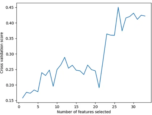
Figure 2 shows the results of the recursive feature elimination process. The plotted scores are the prediction scores (with highest score 1) resulting using cross validation. The highest score is achieved for the subset containing 26 550
features. The 7 features that are eliminated are the following: year the pur-chase order was raised (ranked 2nd); year of delivery accepted by tier 1 supplier (ranked 3rd); order quantity (ranked 4th); part number (ranked 5th); day the purchase order was raised (ranked 6th); the difference between the delivery dates originally requested and accepted by tier 1 supplier (ranked 7th); and day the 555
delivery was due (ranked 8th). For the remainder of this section we present results using both the original 33 features and the 26 remaining features after selection.
Figure 2: Scores for each subset of 33 features
5.2. SVM Models
As mentioned earlier, we conducted grid search using scikit-learn in order 560
to find optimal values for the SVM parameters C and γ. C is the penalty of misclassification, with higher values meaning a higher penalty is imposed, hence the model is stricter. Values ofγexpress the influence that each particular training sample has on the model, with lower values meaning increased influence and higher values meaning less influence. Given the fact that we consider several 565
different metrics, we run grid searches for each metric separately and for both feature sets (with 33 and 26 features).
Figure 3 shows indicative results of the grid search process, using average precision andF1 score as metrics. For average precision, very low C values are
not optimal and results generally improve as values ofγ increase. Highest av-570
erage precision is achieved for C = 1 and γ = 104, which means that, in this
mis-(a) Average Precision with 33 features (b) Average Precision with 26 features
(c)F1 score with 33 features (d)F1 score with 26 features Figure 3: Indicative grid search results for SVM parameters.
Table 1: Prediction scores using SVM and 33 features
Params Test Scores Classification
C γ AP F1 Recall MCC Acc TP TN FP FN
1 104 0.835 0.764 0.712 0.646 0.939 721 6169 155 291
103 103 0.632 0.771 0.740 0.738 0.940 749 6144 180 263
104 103 0.618 0.765 0.766 0.728 0.935 775 6086 238 237
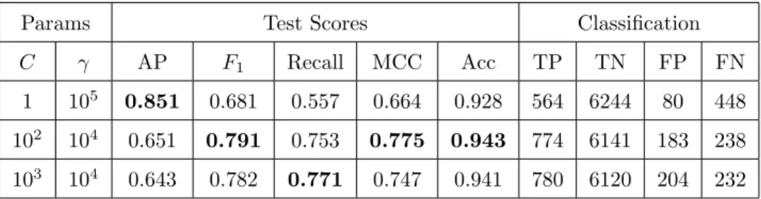
Table 2: Prediction scores using SVM and 26 features
Params Test Scores Classification
C γ AP F1 Recall MCC Acc TP TN FP FN
1 105 0.851 0.681 0.557 0.664 0.928 564 6244 80 448
102 104 0.651 0.791 0.753 0.775 0.943 774 6141 183 238
103 104 0.643 0.782 0.771 0.747 0.941 780 6120 204 232
classification, but by limiting the influence that each sample has on the model. For F1, results are similar, although differences are more pronounced. Scores
are much lower for very low C values and while results improve asγ increases, 575
they actually deteriorate for the highest value (γ = 104). Highest values are
for C = 104 and γ = 104. Since F
1 is the harmonic mean between precision
and recall and given the results on precision, we can draw the conclusion that higher misclassification penalty is required to achieve high recall while main-taining high precision. Results are similar between the two feature sets, with 580
the smaller set achieving higher scores for a slightly higher range of parameters, which confirms the results of the recursive feature elimination process.
As should be expected, different optimal parameters were obtained through the grid search process for each metric and for the two feature sets. Tables 1 and 2 offer a comparison of these results. Each line corresponds to the optimal 585
parameters calculated using one of the metrics. Values in bold are the highest achieved for each metric.
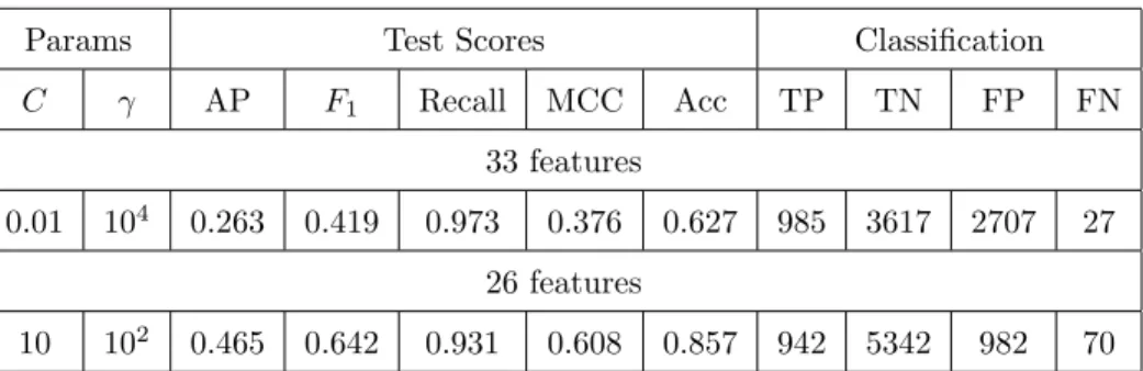
met-Table 3: Prediction scores using random oversampling and SVM
Params Test Scores Classification
C γ AP F1 Recall MCC Acc TP TN FP FN
33 features
0.01 104 0.263 0.419 0.973 0.376 0.627 985 3617 2707 27
26 features
10 102 0.465 0.642 0.931 0.608 0.857 942 5342 982 70
rics, although results are lower for balanced metrics and recall, than average pre-cision. Also, highest values for average precision are achieved for lower penalty 590
values (parameter C), while for all other metrics, higher penalty values are required. The results also show how misleading accuracy can be as a met-ric in scenarios with imbalanced datasets. If read without analysis, accuracy scores indicate that, regardless of parameter values, models are highly success-ful, achieving 94% accuracy. However, if we look at the TP and FN values, 595
the reality is that the best-performing model misses 237/1012 = 23.4% of late delivery cases. This is reflected more accurately in the scores using all other metrics.
Results improve slightly using the features that remain after the feature selection process. Highest MCC score is improved the most, by 5%, while highest 600
recall is almost unchanged. The model with parameters C = 103 and γ = 104achieves the lowest number of false positives, predicting correctly 77.1% of late deliveries. Parameters C = 1 and γ = 105 lead to the highest precision, with 87.6% of predictions of late delivery being correct. Finally, parameters C = 102 and γ = 104 lead to the best possible compromise between different
605
classifications.
Using resampling techniques to tackle data imbalance does not lead to sig-nificant improvements in prediction performance, apart from recall. Table 3 shows the results of using random oversampling before running a grid search optimising recall. While almost perfect recall is achieved for both feature sets 610
Table 4: Prediction scores using decision trees
Test Scores Classification
Features AP F1 Recall MCC Acc TP TN FP FN
33 0.666 0.800 0.817 0.768 0.944 827 6097 227 185
26 0.693 0.816 0.806 0.787 0.949 816 6153 171 196
Table 5: Prediction scores using decision trees with max depth=6 and max leaf nodes=13
Test Scores Classification
Features AP F1 Recall MCC Acc TP TN FP FN
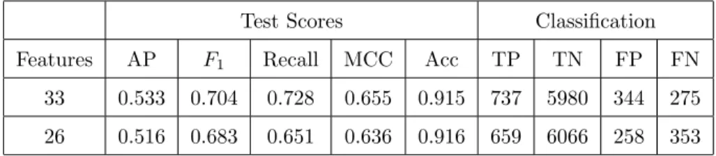
33 0.533 0.704 0.728 0.655 0.915 737 5980 344 275
26 0.516 0.683 0.651 0.636 0.916 659 6066 258 353
(predicting correctly 97.3% and 93.1% of late deliveries using 33 and 26 fea-tures, respectively, it is at the expense of the other metrics. Specifically, for the full feature set, 2707 samples are misclassified as late deliveries, leading to a precision of only 18.5%. For the 26-feature set, results are slightly more bal-anced, with 982 samples misclassified as late deliveries and a precision of 49%. 615
This explains why random oversampling does not improve metrics such as F1
or MCC, since they take into account both false positives and false negatives.
5.3. Decision Tree Models
For decision trees, we first executed the decision tree classifier implemented in scikit-learn with default parameters. This classifier is an optimised version of 620
the CART algorithm uses the gini impurity measure to decide on the quality of each split in the tree: each split must minimise the probability that a random element in the sets created by the split is misclassified if classified according to the label of the majority of the elements. Also, no limit is imposed on the size and structure of the resulting tree. Results using both feature sets are shown 625
in Table 4.
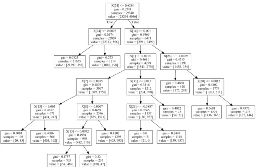
Figure 4: Decision tree classifier using restricted parameters
of average precision but with slightly betterF1 scores. However, the resulting
trees are considerably large: for 33 features the resulting tree has a maximum depth of 29 and 2267 total nodes, while for 26 features depth is 28 and total 630
nodes are 2401. Since interpretability is hindered when trees grow too large, we limited the classifier to a maximum depth of 6 and maximum 13 leaf nodes. This led to trees with 25 nodes in total, such as the one in Figure 4. Results using restricted parameters are shown in Table 5.
In the tree shown in Figure 4 the feature that contributes to the best split 635
(X[24]) is the difference between the due date of the delivery and the date that was accepted by the tier 1 supplier. This leads to roughly 78% of the training samples classified as not late if the difference is less than or equal to 21 days (the value corresponding to 0.0022 before normalisation), which is incorrect for only 556 samples. For the remaining 23% the decision depends on combinations 640
of additional features. For instance, when the season of the due date is not winter (corresponding to taking the left branch at node whereX[14]≤0.001), the purchase order month is January to June (left branch ofX[1]≤0.0015), the
Table 6: Prediction scores using random oversampling and decision trees
Test Scores Classification
Features AP F1 Recall MCC Acc TP TN FP FN
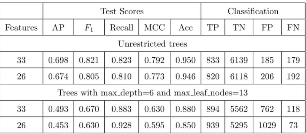
Unrestricted trees
33 0.698 0.821 0.823 0.792 0.950 833 6139 185 179
26 0.674 0.805 0.810 0.773 0.946 820 6118 206 192
Trees with max depth=6 and max leaf nodes=13
33 0.493 0.670 0.883 0.630 0.880 894 5562 762 118
26 0.453 0.630 0.928 0.595 0.850 939 5295 1029 73
date that was accepted by the tier 1 supplier is not in the last 9 weeks of the year (left branch ofX[31]≤0.012) and the delivery date originally requested by 645
the tier 1 supplier is within a year of the currently accepted one (right branch ofX[26]≤ −0.3887), then the delivery is predicted to be late. This is correct for 957 of the 1116 samples.
Using resampling techniques in combination with decision trees yields a mix-ture of results. For unrestricted decision trees, prediction performance is slightly 650
improved overall for 33 features but is slightly lower for 26 features. In both cases, trees are significantly larger than without random oversampling: depth of 36 and 2711 nodes for 33 features and depth of 37 and 2681 nodes for 26 fea-tures. For decision trees restricted to a maximum depth of 6 and maximum 13 leaf nodes, results are similar to SVM: recall is significantly improved for both 655
33 and 26 features, at the expense of the other metrics. Results are summarised in Table 6.
6. Discussion
In this section we discuss the presented results in relation to interpretability and dataset characteristics. Section 6.1 discusses the tradeoff between predic-660
tion performance and interpretability, as well as the potential knowledge that can be gained from interpretable models to influence SCRM processes. Then,
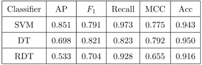
Table 7: Summary of best prediction scores for different classifiers and metrics
Classifier AP F1 Recall MCC Acc
SVM 0.851 0.791 0.973 0.775 0.943
DT 0.698 0.821 0.823 0.792 0.950
RDT 0.533 0.704 0.928 0.655 0.916
Section 6.2 summarises the effects of feature engineering and selection, as well as data imbalance, as perceived in the presented case study. To facilitate dis-cussion, Table 7 contains only the best scores, from the ones reported in the 665
tables of Section 5, that were achieved for each metric using SVM, unrestricted decision trees (DT) and restricted decision trees (RDT).
6.1. Interpretability
Results in Table 7 show that decision trees without restrictions are capa-ble of achieving comparacapa-ble results with SVM, performing slightly worse with 670
regard to average precision and recall but doing slightly better in the case of balanced metrics, F1 score and MCC. Imposing restrictions on decision trees
helps quantify the trade-off between performance and interpretability. For the particular dataset, a classifier whose results can be easily interpreted achieves 37% lower average precision, 15% lower MCC score, 11% lowerF1score and 5%
675
lower recall.
The question that the SCRM decision-makers have to consider is whether the potentially lower performance of interpretable models is acceptable, given the fact that predictions can be interpreted. The decision is case-specific and is entirely dependent to the particular set of data, SCRM plan and prediction 680
priorities. If, for instance, the importance placed on precision is high because there are significant costs in treating a delivery as late when this will not be the case eventually, then the added value of interpretability may be less appealing. If, on the other hand, the primary goal of the SCRM plan is to understand what factors may contribute more to a delivery being late, then some reduction in 685
prediction performance may be deemed acceptable.
With regard to knowledge that can be gained from interpretable machine learning models, the presented case study shows that decision trees can be informative, revealing correlations of feature values that lead to one or the other outcome. Decision trees by design can deliver such interpretation, whereas this 690
is not possible with SVM models. The particular dataset and features could only yield mainly date-related information, but richer datasets could potentially be even more helpful. This knowledge about correlation patterns in the dataset can then be taken into account in SCRM decision-making efforts, keeping in mind that correlation does not necessarily imply causality. The importance of 695
tree depth should also be obvious by this example: explaining decisions starts becoming too complex after 4 or 5 splits.
6.2. Datasets and Imbalance
The importance of a feature-rich dataset is also illustrated in the presented case study. The feature engineering process yielded additional features based 700
on date-related information; however, further feature combinations were not possible, since the initial feature set was quite limited. Also, feature selection in such a dataset does not lead to significant improvement in performance; however, it can definitely prove useful in identifying the most important features and reducing the size of the feature set to increase execution time for complex 705
tasks such as grid search for SVM.
Finally, the significant effect of imbalanced datasets is evident throughout the presented results, especially with regard to performance metrics. Accuracy is proven to be not only uninformative but potentially misleading. Balanced metrics such asF1 and MCC scores present a more conservative but fair
evalu-710
ation of prediction performance. However, no one metric is the best choice for any SCRM prediction task: it is the task and particularly the goals set within the SCRM planning process that should lead to the correct choice of metrics. As in the case study, recall is more useful when the goal is to minimise missed cases of late delivery, while precision is preferable when incorrectly predicting 715
a delivery to be late is especially undesirable. These considerations should be taken into account in any SCRM-related prediction effort that involves events and risks that are less likely to occur.
7. Conclusions and Future Work
In this work, we proposed a risk prediction framework for SCRM that utilises 720
data-driven AI techniques and relies on the collaboration and interactivity be-tween AI and supply chain experts. The framework emphasises the need for linking choices of metrics and algorithms to SCRM goals which may prioritise interpretability over prediction performance or vice-versa. It also illustrates the difficulties of working with imbalanced datasets, which may feature in SCRM-725
related scenarios. The applicability of the framework is demonstrated through a real-world case study of a multi-tier aerospace manufacturing supply chain af-fected by the risk of delayed deliveries. Results of experiments conducted within the case study show that the framework can achieve good performance across a variety of metrics using both black box and interpretable machine learning 730
techniques. Prioritising interpretability over performance requires a compro-mise that is minor in terms of recall (5% decrease in prediction performance) but much higher in terms of average precision (37% decrease).
Future research directions on the application of AI techniques in SCRM include: (a) exploring a more feature-rich dataset and a larger set of ma-735
chine learning techniques, including, for instance, neural networks and deep learning, and their effects on interpretability and performance; (b) extracting knowledge through a combination of data-driven and knowledge-based AI tech-niques [37, 38] and using it to derive managerial insights and influence sup-ply chain decision-making processes; and (c) investigating whether similar ap-740
proaches can be applied in other phases of the SCRM process, such as risk assessment and response.
References
[1] M. S. Sodhi, B.-G. Son, C. S. Tang, Researchers’ Perspectives on Supply Chain Risk Management, Production and Operations Management 21 (1) 745
(2012) 1–13.
[2] G. Baryannis, S. Validi, S. Dani, G. Antoniou, Supply chain risk manage-ment and artificial intelligence: state of the art and future research direc-tions, International Journal of Production Research 57 (7) (2019) 2179– 2202. doi:10.1080/00207543.2018.1530476.
750
[3] T. L. Saaty, The analytic hierarchy process : planning, priority setting, re-source allocation, McGraw-Hill International Book Co., New York; London, 1980.
[4] A. Charnes, W. Cooper, E. Rhodes, Measuring the efficiency of decision making units, European Journal of Operational Research 2 (6) (1978) 429 755
– 444.
[5] G. Baryannis, S. Dani, S. Validi, G. Antoniou, Decision Support Systems and Artificial Intelligence in Supply Chain Risk Management, in: G. A. Zsidisin, M. Henke (Eds.), Revisiting Supply Chain Risk, Springer Series in Supply Chain Management, Springer International Publishing, 2019, pp. 760
53–71. doi:10.1007/978-3-030-03813-7_4.
[6] Y. Fan, L. Heilig, S. Voss, Supply chain risk management in the era of big data, Lecture Notes in Computer Science 9186 (2015) 283–294. doi: 10.1007/978-3-319-20886-2_27.
[7] M. He, H. Ji, Q. Wang, C. Ren, R. Lougee, Big data fueled process man-765
agement of supply risks: Sensing, prediction, evaluation and mitigation, in: Proceedings - Winter Simulation Conference, Vol. 2015-January, IEEE, Sa-vanah, GA, USA, 2015, pp. 1005–1013. doi:10.1109/WSC.2014.7019960. [8] D. Zage, K. Glass, R. Colbaugh, Improving supply chain security using big data, in: 2013 IEEE International Conference on Intelligence and Security 770
Informatics: Big Data, Emergent Threats, and Decision-Making in Security Informatics, IEEE, Seattle, WA, USA, 2013, pp. 254–259. doi:10.1109/ ISI.2013.6578830.
[9] S. Ye, Z. Xiao, G. Zhu, Identification of supply chain disruptions with eco-nomic performance of firms using multi-category support vector machines, 775
International Journal of Production Research 53 (10) (2015) 3086–3103.
doi:10.1080/00207543.2014.974838.
[10] F. Doshi-Velez, B. Kim, Towards a rigorous science of interpretable machine learning, arXiv preprint arXiv:1702.08608.
[11] P. M. Domingos, A Few Useful Things to Know about Machine Learning., 780
Commun. ACM 55 (10) (2012) 78–87.
[12] C. Molnar, Interpretable Machine Learning,
https://christophm.github.io/interpretable-ml-book/, 2019.
[13] V. Mani, C. Delgado, B. Hazen, P. Patel, Mitigating supply chain risk via sustainability using big data analytics: Evidence from the manufacturing 785
supply chain, Sustainability 9 (4) (2017) N/A. doi:10.3390/su9040608. [14] A. Bruzzone, A. Orsoni, AI and simulation-based techniques for the
as-sessment of supply chain logistic performance, in: 36th Annual Simu-lation Symposium, IEEE, Orlando, FL, USA, USA, 2003, pp. 154–164.
doi:10.1109/SIMSYM.2003.1192809. 790
[15] L. Zhang, X. Wu, M. J. Skibniewski, J. Zhong, Y. Lu, Bayesian-network-based safety risk analysis in construction projects, Reliability Engineering & System Safety 131 (2014) 29 – 39. doi:10.1016/j.ress.2014.06.006. [16] S.-S. Leu, C.-M. Chang, Bayesian-network-based safety risk assessment for steel construction projects, Accident Analysis & Prevention 54 (2013) 122 795
[17] M. Garvey, S. Carnovale, S. Yeniyurt, An analytical framework for supply network risk propagation: A Bayesian network approach, European Journal of Operational Research 243 (2) (2015) 618–627. doi:10.1016/j.ejor. 2014.10.034.
800
[18] R. Ojha, A. Ghadge, M. K. Tiwari, U. S. Bititci, Bayesian network mod-elling for supply chain risk propagation, International Journal of Produc-tion Research 0 (0) (2018) 1–25. doi:10.1080/00207543.2018.1467059. [19] Y. Shang, D. Dunson, J.-S. Song, Exploiting big data in logistics risk
as-sessment via Bayesian nonparametrics, Operations Research 65 (6) (2017) 805
1574–1588. doi:10.1287/opre.2017.1612.
[20] T. Papadopoulos, A. Gunasekaran, R. Dubey, N. Altay, S. J. Childe, S. Fosso-Wamba, The role of big data in explaining disaster resilience in supply chains for sustainability, Journal of Cleaner Production 142 (2017) 1108 – 1118. doi:10.1016/j.jclepro.2016.03.059.
810
[21] D. Li, X. Wang, Dynamic supply chain decisions based on networked sensor data: an application in the chilled food retail chain, International Journal of Production Research 55 (17) (2017) 5127–5141. doi:10.1080/00207543. 2015.1047976.
[22] M. Chen, Y. Xia, X. Wang, Managing supply uncertainties through 815
Bayesian information update, IEEE Transactions on Automation Science and Engineering 7 (1) (2010) 24–36. doi:10.1109/TASE.2009.2018466. [23] K. Zhao, X. Yu, A case based reasoning approach on supplier selection
in petroleum enterprises, Expert Systems with Applications 38 (6) (2011) 6839–6847. doi:10.1016/j.eswa.2010.12.055.
820
[24] C. Martin, H. Peck, Building the resilient supply chain, The International Journal of Logistics Management 15 (2) (2004) 1–14.
[25] E. Alpaydin, Introduction to machine learning, 3rd Edition, MIT press, 2014.
[26] D. Bellman, Dynamic Programming, Princeton University Press, 1957. 825
[27] T. G. Dietterich, Overfitting and undercomputing in machine learning., ACM Comput. Surv. 27 (3) (1995) 326–327.
[28] H. He, E. Garcia, Learning from Imbalanced Data, IEEE Transactions on Knowledge and Data Engineering 21 (9) (2009) 1263–1284. doi:10.1109/ TKDE.2008.239.
830
[29] F. Pedregosa, G. Varoquaux, A. Gramfort, V. Michel, B. Thirion, O. Grisel, M. Blondel, P. Prettenhofer, R. Weiss, V. Dubourg, J. Vanderplas, A. Pas-sos, D. Cournapeau, M. Brucher, M. Perrot, E. Duchesnay, Scikit-learn: Machine Learning in Python, Journal of Machine Learning Research 12 (2011) 2825–2830.
835
[30] G. Lemaˆıtre, F. Nogueira, C. K. Aridas, Imbalanced-learn: A python tool-box to tackle the curse of imbalanced datasets in machine learning, Journal of Machine Learning Research 18 (17) (2017) 1–5.
URLhttp://jmlr.org/papers/v18/16-365.html
[31] S. Boughorbel, F. Jarray, M. El-Anbari, Optimal classifier for imbalanced 840
data using matthews correlation coefficient metric, PLOS ONE 12 (6) (2017) 1–17. doi:10.1371/journal.pone.0177678.
[32] K. P. Bennett, C. Campbell, Support vector machines: Hype or hallelujah?, SIGKDD Explor. Newsl. 2 (2) (2000) 1–13. doi:10.1145/380995.380999. [33] N. Chawla, K. Bowyer, L. Hall, W. Kegelmeyer, SMOTE: Synthetic Mi-845
nority Over-sampling Technique, Journal of Artificial Intelligence Research 16 (2002) 321–357.
[34] H. He, Y. Bai, E. A. Garcia, S. Li, ADASYN: Adaptive synthetic sampling approach for imbalanced learning., in: IJCNN, IEEE, 2008, pp. 1322–1328. [35] I. Tomek, Two Modifications of CNN, IEEE Transactions on Systems, Man, 850
[36] G. E. A. P. A. Batista, R. C. Prati, M. C. Monard, A study of the behavior of several methods for balancing machine learning training data., SIGKDD Explorations 6 (1) (2004) 20–29.
[37] G. Baryannis, D. Plexousakis, Fluent Calculus-based Semantic Web Service 855
Composition and Verification using WSSL, in: A. Lomuscio, et al. (Eds.), 9th International Workshop on Semantic Web Enabled Software Engineer-ing (SWESE2013), co-located with ICSOC 2013, Vol. 8377 of Lecture Notes in Computer Science, Springer International Publishing Switzerland, 2014, pp. 256–270. doi:10.1007/978-3-319-06859-6_23.
860
[38] G. Baryannis, D. Plexousakis, WSSL: A Fluent Calculus-Based Language for Web Service Specifications, in: C. Salinesi, M. C. Norrie, ´O. Pas-tor (Eds.), 25th International Conference on Advanced Information Sys-tems Engineering (CAiSE 2013), Vol. 7908 of Lecture Notes in Computer Science, Springer Berlin Heidelberg, 2013, pp. 256–271. doi:10.1007/
865