The Synchronous
Programming Language
Quartz
A Model-Based Approach to the Synthesis of
Hardware-Software Systems
November 13, 2010, Version 2.0
Department of Computer Science
University of Kaiserslautern
1 Introduction. . . 1
1.1 Embedded System Design . . . 1
1.2 Models of Concurrent Computation . . . 4
1.3 Model-based Design Methods . . . 12
1.3.1 High-level Synthesis . . . 12
1.3.2 Software Synthesis for Embedded Systems. . . 12
1.3.3 Latency-Insensitive Implementations. . . 12
2 Data Types, Expressions, and Specifications . . . 13
2.1 Data Types . . . 14
2.1.1 Syntax and Semantics of Data Types . . . 14
2.1.2 Matching Types to Expected Supertypes . . . 16
2.1.3 Primitive Recursive Data Types . . . 17
2.2 Expressions. . . 17
2.2.1 Variables . . . 18
2.2.2 Literals. . . 19
2.2.3 Operators . . . 21
2.2.4 Static (i.e. Compile-time Constant) Expressions. . . 32
2.2.5 User-Defined Functions. . . 33
2.3 Specifications . . . 33
2.3.1 Syntax. . . 34
2.3.2 Type Rules. . . 37
2.3.3 Semantics. . . 39
3 Statements, Interfaces and Modules . . . 43
3.1 Modules and Interface Declarations . . . 45
3.1.1 Interface Declarations. . . 45
3.1.2 Statements . . . 49
3.2 Semantic Problems . . . 58
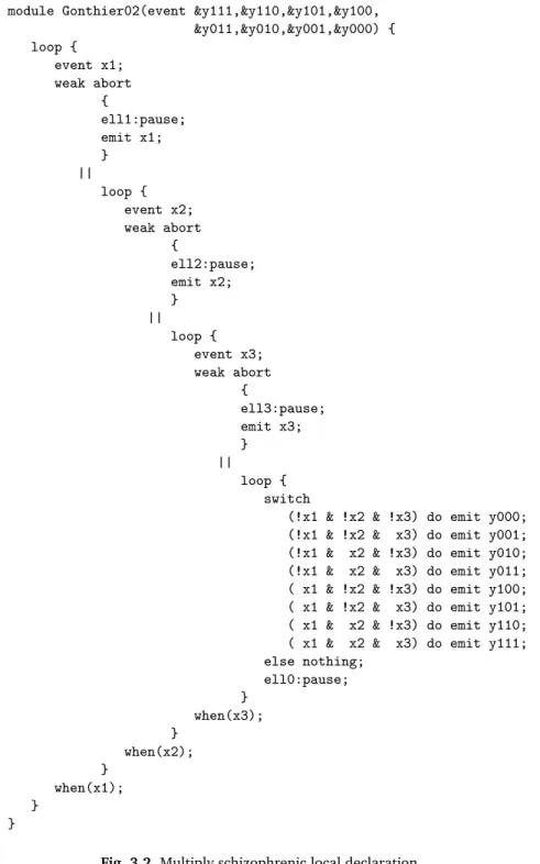
3.2.1 Schizophrenic Statements . . . 58
3.3 Core Statements. . . 67
3.4 Macro Statements . . . 69
3.4.1 Simple Macro Statements. . . 69
3.4.2 Additional Wait-Statements. . . 70
3.4.3 Additional Loops . . . 70
3.4.4 Additional During-Statements. . . 70
3.4.5 Let-Abbreviations. . . 70
3.4.6 Conjunctively Active Parallel Execution. . . 71
3.4.7 Generic Sequence and Parallel Statements . . . 71
3.4.8 Delay Statements . . . 72
3.4.9 Abstractions . . . 72
3.4.10 Nondeterminism and Asynchronous Concurrency . . . 73
3.4.11 Exception Handling. . . 75
3.4.12 Micro Step Variables. . . 81
3.4.13 Inout Variables. . . 81
4 Formal Semantics . . . 83
4.1 Evaluating Expressions in Incomplete Environments. . . 86
4.2 SOS Transition Rules. . . 88
4.3 SOS Reaction Rules (Causality Analysis) . . . 97
4.4 Complete Operational Semantics . . . 102
4.5 Symbolic SOS Transition Rules: The Control Flow Predicates . . 106
4.5.1 Computing the Control Flow. . . 108
4.5.2 Computing Guarded Actions . . . 115
4.5.3 Computing the Data Flow . . . 124
4.5.4 Haltset Encoding of Symbolic SOS Rules. . . 127
4.6 Symbolic SOS Reaction Rules . . . 130
4.6.1 Causality Analysis with Higher Data Types . . . 130
4.6.2 Can- and Must-Guarded Actions. . . 139
5 Compilation to Guarded Actions. . . .145
5.1 Revisiting Schizophrenia Problems. . . 147
5.2 Translation to Guarded Actions. . . 150
5.2.1 Computing Guarded Actions of the Surface . . . 151
5.2.2 Computing Guarded Actions of the Depth. . . 161
5.3 Overall Compilation and Linking. . . 170
6 Synthesis of Synchronous Systems. . . .179
6.1 Synthesis of Data Flow Equations. . . 179
6.1.1 Equation Systems as Hardware Circuits. . . 184
6.2 Software Synthesis based on Explicit Extended Finite State Machines. . . 188
6.3 Software Synthesis based on Equation Systems . . . 188
6.3.1 Dataflow Evaluation of Equation Systems. . . 189
6.3.3 Dataflow Evaluation and Multithreaded Execution . . . 190
6.3.4 Dataflow Evaluation and Constructive Programs. . . 191
6.3.5 Adjusting the Granularity by Macro Nodes . . . 194
6.4 Compiling Synchronous Programs into Graph Code . . . 195
6.5 Compiling Synchronous Programs into Jobs. . . 195
6.6 Formal Semantics of the Job Code . . . 197
6.6.1 Approximating the Environment. . . 198
6.6.2 Preparing the Next Macro Step. . . 199
7 Synthesis of Asynchronous Systems. . . .211
7.1 Dataflow Process Networks . . . 215
7.1.1 Syntax of DPNs . . . 215
7.1.2 Denotational Semantics of DPNs. . . 219
7.1.3 DPNs as Rewrite Systems. . . 223
7.1.4 Operational Semantics of DPNs. . . 230
7.1.5 The Full Abstraction Problem . . . 238
7.1.6 The Kahn Principle . . . 241
7.2 Important Classes of Dataflow Process Networks. . . 241
7.2.1 Single-Rate Dataflow Process Networks. . . 241
7.2.2 Synchronous Dataflow Process Networks . . . 242
7.2.3 Cyclo-Static Dataflow Process Networks . . . 248
7.2.4 Boolean Dataflow Process Networks. . . 251
7.2.5 Tagged Dataflow Process Networks . . . 251
7.3 Globally Asynchronous Locally Synchronous Systems. . . 251
7.3.1 Synchronous Programs vs. Dataflow Programs. . . 251
7.3.2 Endochrony and Isochrony. . . 259
7.3.3 Weak Endochrony . . . 286
7.3.4 Elastic Synchronous Systems. . . 293
8 Sanity Checks. . . .295
8.1 Surface-Depth Expansion of Statements . . . 295
8.1.1 Surface/Depth-Splitting withoutgoto . . . 298
8.1.2 Surface/Depth-Splitting withgoto. . . 309
8.2 Formal Verification of Properties. . . 316
8.2.1 From Assumptions and Assertions to Specifications. . . 316
8.2.2 Model Checking of Temporal Logics. . . 316
8.2.3 Supervisory Control (Reactive Synthesis) . . . 316
8.3 Checking Absence of Overflows. . . 316
8.4 Checking Absence of Write Conflicts. . . 316
8.4.1 Deadend States and Write Conflicts . . . 317
9 Hardware-Software Codesign . . . .327
9.1 Introduction . . . 327
9.2 Application-Specific Microprocessors . . . 327
9.3 Dynamically Reconfigurable Processing Elements . . . 327
9.4 HW/SW-Codesign based on Virtual Platforms. . . 327
A Partial Orders. . . .329
A.1 Complete Partial Orders . . . 329
A.1.1 Partial Orders and Directed Subsets. . . 329
A.1.2 Complete Partial Orders. . . 333
A.1.3 Fixpoint Theorems. . . 335
A.1.4 Cartesian Products of Partial Orders. . . 340
A.2 Complete Lattices. . . 343
A.2.1 Lattices . . . 343
A.2.2 Complete Lattices . . . 345
A.3 Theory of Streams . . . 348
A.3.1 Complete Partial Order of Streams. . . 348
A.3.2 Metric Space of Streams. . . 352
B Computer Arithmetic. . . .357 B.1 Natural Numbers. . . 358 B.2 Radix-BNumbers . . . 362 B.3 The Integers . . . 389 B.4 B-Complement Numbers . . . 391 B.5 Hardware-Implementations. . . 409 B.5.1 Radix-2 Arithmetic . . . 409 B.5.2 2-Complement Arithmetic . . . 415
B.6 Further Representations of Numbers . . . 417
B.6.1 Gray Code Numbers . . . 419
B.6.2 Residue Number Systems. . . 419
B.6.3 Signed Digit Numbers. . . 419
C Concrete Grammar of the Quartz Language . . . .421
C.1 Lexical Tokens . . . 421
C.2 Grammar of the Quartz Language. . . 423
C.3 Some Example Programs . . . 427
References . . . .429
Introduction
1.1 Embedded System Design
During the past decades, an incredible change of technology has been ob-served in many devices: traditionally used mechanical parts have often been first replaced by analog electronic devices, then by digital hardware, and later on by programmable microprocessors. Finally, entire computer systems con-sisting of a microprocessor with a main memory and specific input/output fa-cilities running some application-specific software have been integrated which lead to the definition ofembedded systems. One of the first embedded systems was probably the Apollo guidance computer [187] for navigation and control of the Apollo spacecrafts designed in the 1960s. They were considered the most risky parts of the Apollo project.
The use of embedded systems has many advantages: it allowed not only a cheaper production, it also allowed the miniaturization of devices and the integration of more intelligent functionalities. The increased use of software makes embedded system more flexible so that late changes in their design are manageable and even changes after shipping these systems are possible.
Today, the progress in technology is still unbroken, and there is now a trend towards the integration of more processors on a single chip, so that evenheterogeneous multiprocessor systems on a single chip (MPSoCs) can be used for the design of embedded systems. The combination of a dynamically scheduled general purpose RISC CPU with a statically scheduled VLIW/DSP processor is often viewed classic in some application areas. The use of MP-SoCs often allows the tenfold increase in computing power with a tenfold decrease of energy consumption. Huge markets like those for mobile phones or other consumer electronics lead to mass production that made prices for simple microprocessors about one dollar possible. Other important applica-tion areas of embedded systems are avionics and automotive industries (e.g. anti-lock braking system (ABS), electronic stability control (ESC/ESP), trac-tion control (TCS) and automatic four-wheel drive), consumer electronics, CD/DVD/BlueRay players, domestic appliances, communication devices,
traf-fic control systems including navigation devices, controllers for industrial plants, and special devices used in medical equipments (pacemakers, PET, CT).
Unfortunately, thedesign of embedded systems[176] is still not well devel-oped. One problem is thatmany different disciplineslike software engineering, hardware design, control theory as well as mechanical and electrical engineer-ing are involved that have not yet been integrated into a seamless design flow. Another problem is that evennew solutions within these disciplineshave to be developed to address the special needs of embedded systems. To discuss these issues in software and hardware synthesis for embedded systems that lead to the motivation of new programming languages like synchronous languages, we have to consider the general architecture of embedded systems.
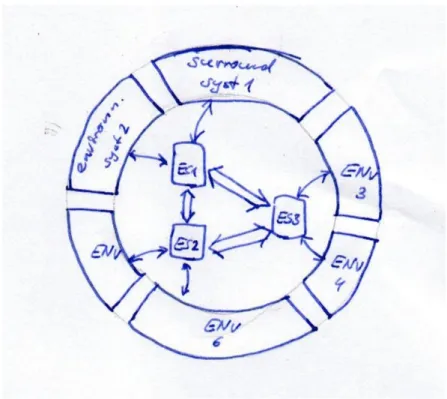
Fig. 1.1.General Architecture of an Embedded System
The general architecture of an embedded systemis shown in Figure 1.1: The embedded system itself may consist of many subsystems each consisting of multiple processors running application-specific software. These computer systems communicate not only with themselves but also directly with their environment. From the technological side, analog-digital converters used in special sensors and actor may be used for the communication between the
environment and the embedded system, and special bus systems [220] like CAN, FlexRay, MOST, LIN are used for the communication of the embedded systems with each other. The communication of single subsystems within one embedded system are supported by special busses like ARM’s AMBA bus. Each of the embedded system consists of software and hardware, where the hard-ware is furthermore divided into a part consisting of standard components such as micro-processors and special components that are implemented for a particular application. A new emerging trend is also the use of application-specific processors whose instruction sets are adapted to a particular applica-tion. Hence, beingapplication-specific computer systemsis already a character-izing property of embedded systems.
The communication of the embedded systems with their environment leads to further properties. Unlike classic (transformational) software pro-grams that read inputs at starting time and produce outputs at termination time, many embedded systems are so-called reactive systems as introduced by Harel and Pnueli [122]. Like interactive systems, reactive systems have an ongoing communication with their environment, but in contrast to inter-active systems, reinter-active systems have to respond to the events generated by their environment at the points of time determined by the environment. For this reason, reactive systems are special kinds ofreal-time systemsso that not only special real-time operating systems are used, but also theworst-case exe-cution/reaction timehas to be estimated for these systems.
Since embedded systems were used in safety-critical areas from their be-ginning, the design flows must take special care on the correctness of the software and hardware developed for such systems.Formal verificationis one of the success stories of modern computer science, where in particular model checking makes it now possible to completely verify considerably large sys-tems using sophisticated techniques like symbolic state space representations and various kinds of abstractions. It is therefore mandatory that a design flow covers formal verification and to this end, used languages must have a formal semantics that allows a direct translation to state transition systems as used by modern verification methods.
Like essentially all computer systems today, also the hardware of embed-ded systems is digital, so that their modeling as discrete state transition sys-tems is adequate. However, the environment of embedded syssys-tems is often continuous. Hence, to argue about the effects on the physical environment, one has to consider the entire system which is ahybrid system[7,125,126]. In these systems, the state of the environment is determined by differential equations that determine the continuous change of variables describing the environment’s behavior, while the states of the embedded system are dis-crete. The state transitions of the embedded system may lead to changes of the differential equations, and therefore may influence the environment of the embedded system, while the values of the continuous inputs to the em-bedded system may influence their state transitions. A holistic consideration
of embedded systems must therefore not necessarily be able to synthesize mixed-signal systems, but it must be able to simulate and verify such systems.
1.2 Models of Concurrent Computation
Traditional programming languages miss several features that are of essential importance for the design of reactive real-time systems. In particular, anotion of time and concurrencyis required as well as special data types to distinguish between events and stored values. For this reason, many new languages have been proposed that provide such features. However, only a few of these lan-guages allow both the synthesis of hardware as well as software from the same program, and only a few of them allow a translation to state transition systems as required for most formal verification methods.
In order to classify different kinds of programming languages and mod-eling styles, models of concurrent computation have been introduced [109, 133, 165?, 166]. Being more abstract as programming languages, a model of concurrent computation has to determine what triggers the execution of a concurrent action and how do concurrent parts of a system communicate with each other.
Among many different models of computation, the most important ones are the following ones:
Event-Triggered Languages
The computation ofdiscrete event systems[67] is triggered by the occurrence of an event, which may be the change of a variable’s value, the satisfiability of a desired condition, or the reaching of a desired point of time. Most hard-ware description languages including VHDL [132], Verilog [130, 179] and SystemC [131] are based on this model of computation, which is best suited for simulation.
Languages that are based on the this model of computation typically con-sist of several sequential processes that are statically defined. The semantics is thereby given by the definition of a simulator that consists of the following phases which define this model of computation:
1. In a firstelaboration phase, the active processes are executed until some form of a wait statement is reached. During this elaboration phase, all val-ues for the assignments to variables are determined in the current variable environment, but the values are not yet assigned. Instead, they are main-tained in a schedule where the assignments are scheduled at a explicit point of (potentially physical) time.
2. After all processes have been elaborated in a simulation cycle, the assign-ments scheduled to the current point of time are synchronously executed in anupdate phase. The possible changes of variable’s values lead to events
that may trigger the further execution of processes at the same point of time.
3. The final step is theevent detection phase: If some variable’s values have been updated, the next simulation cycle takes place at the same point of (physical time), since new events occurred for the current point of time. Otherwise, the point of time for the next simulation cycle is determined by the next point of time in the schedule where assignments should be executed. The next simulation cycle repeats then these steps for the de-termined point of time until the schedule becomes empty.
The advantage of the above model of computation is that it provides a deter-ministic form of concurrency: Since the elaboration phase is performed in the same variable environment, the ordering of processes to be elaborated does not matter and potential write conflicts are detected in the update phase.
As any model of computation, there are some intrinsic semantic problems that lead to undesired behaviors or a lack of behavior. In case of discrete event systems, there may be no progress in physical time, since the processes may generate infinitely many events on the current point of time. Moreover, processes may get stuck in infinite loops, which can however be avoided by certain restrictions of the grammars (to demand the execution of wait state-ments in each loop). Moreover, it can be the case that the schedule requires unbounded memory since processes generate events for later points of time.
Discrete-event based languages lend themselves well for simulation, since the semantics already defines an efficient simulator that executes exactly the necessary changes per execution cycle. However, a synthesis for synchronous hardware circuits is not straightforward unless some restrictions are obeyed. A synthesis of multithreaded software, on the other hand, is straightforward, since the elaboration phase of the processes can be directly implemented by different software threads.
Dataflow Process Networks and CSP
Another model of computation is given by dataflow process networks [138, 139, 141, 164]. Such a network consists of a directed graph whose nodes are associated with simple functions that take some input values from their incoming arcs and produce output values that are put on their outgoing arcs (see Figure1.2). Thefiring of the nodes is possible whenever the required data values are available on its incoming arcs. Depending on the state of the process node, and the current input values, it may be necessary that more than one value is required on one input arc, while it may also be possible that no input value is consumed from another arc. The arcs connecting the process nodes are viewed as unbounded FIFO buffers, so that outputs can always be written to these buffers.
For example, considerBerry’s Gustave function that requires three input arcs x1, x2, andx3 with boolean values and generates boolean values on a single output arcy. The firing rules of this function are defined as follows:
Fig. 1.2.Example of a Dataflow Process Network
x1x2x3 y 0 1 ∗ 1 1 ∗ 0 1 ∗ 0 1 1
As can be seen by the above table, a node associated with the Gustave function can fire in the three listed cases, and in each case, it produces the same output value on the output arcy. For example, this means, the node can fire ifx1and x2hold the values0 and1, respectively, while the content ofx3is irrelevant (it is not read, and therefore, not modified in this case).
As another example, consider a node with the following firing rules: x1 x2 x3 y
0 (a, b) ∗ a+b 1 a b a−b
Depending on the value read from the input bufferx1, either two values must be read fromx2to generate their sum as output value, or a single value has to be read from each of the input buffersx2 andx3to generate their difference as output value. In this node, the number of data values consumed depends on one of the input values, so that the node is adynamic dataflow process.
Since the firing of the single process nodes may not be determined in a fixed schedule at compile time, it is usually not controlled by a central control unit. Instead, each process node has to check its input buffers for available data to fire. Therefore, the execution of the entire process network may not be deterministic in that the points of time where output values are generated may not be known in advance. Nevertheless, it is still desirable that the se-mantics of a dataflow process networkshould be a function, i.e., deterministic. This semantics is defined as a stream processing function that maps the input
data streams to output data streams. A stream is thereby either a finite or in-finite sequence of values of a certain type. Hence, ifDdenotes the set of data values1,Dωdenotes the set of finite and infinite sequences overD, then the
semantics of a dataflow process network is a function of type(Dω)m→(Dω)n.
The definition of the semantics of a process network is however not that simple, since outputs may be fed back as inputs to the process network. For this reason, the output streams are only incrementally computed which makes it difficult to reason about the determinism of a process network. One there-fore considers the prefix ordering of streams where two streams σ1, σ2 are orderedσ1σ2iff eitherσ1=σ2orσ1is a finite prefix ofσ2. It is easily seen that the set of streams forms acomplete partial order with the prefix ordering. Based on the prefix ordering of streams, one can easily define monotonic and continuous stream processing functions: a functionf is monotonic iffσ1σ2 impliesf(σ1)f(σ2), andf is continuous ifff(sup(M)) =sup(f)(M)holds for every nonempty directed2setM. Then, the entire behavior of a dataflow process network can be determined as aleast fixpointof the functions attached to the single process nodes [138,139,241,243] which is known as the Kahn principle [138, 139]. Such a fixpoint exists for all continuous functions, so that determinism follows by the continuity of the functions implemented by the single process nodes.
In practice, one often imposes stronger requirements than continuity like blocking-readand lack of emptiness test of input buffers.Testing the emptiness of an input buffer to determine the output of a node is bad, since the node can-not distinguish whether that input stream was finite and has been completely read or whether further input values will arrive, but have not yet arrived. If a read operation to an input buffer is not blocking, it can be used to implement an emptiness test, which is bad for the above reason. Forbidding both empti-ness test and unblocking-read guarantees continuous functions, and therefore a deterministic semantics of the dataflow process network.
It is however known that there are continuous functions that do not ful-fill these stronger requirements: For example, the above mentioned Gustave function is continuous, but can obviously not be implemented by a blocking-read policy (since it may be the case that one unfortunately tries to blocking-read an input streamxi that carries no further values). In practice, the blocking-read
policy and the lack of emptiness test is however sufficient.
An advantage of Kahn process networks is that theirbehaviors can be in-crementally computed: First, continuous functions are monotonic, and second, due to Bekic’s lemma, it does not matter whether we proceed faster or slower with the consumption of values of the one or the other input stream.
Vuillemin strengthens the notion of continuous function tosequential func-tions[164,189,258]. Formally, a functionf : (Dω)m →(Dω)n is sequential
1We ignore different types in this formulation. 2A set
M is directed iff for two elementsx, y∈M, there is an elementz∈M such thatxzandyz.
if it is continuous and for all input streams σ1, . . . , σm ∈ Dω, there is an
i∈ {1, . . . , m}such that for all extended input streamsσ10, . . . ,σ0m∈ Dωwith
σj σ0j forj 6=iandσi σ0i, we havef(σ1, . . . , σm) =f(σ10, . . . , σ0m). This
means that the computation of the output streams off can not proceed until a new value is received from input streamσi. In practice, this means that for
a sequential function, one knows at every point of time due to the so-far read input sequences which value has to be read next from which input buffer. This means, for each sequential function, we can start reading its arguments from certain input buffers, and depending on their values, we go on by read-ing some other channels etc. until all values have been read to compute the current reaction. For example, an if-then-else node is sequential in that it first reads the condition value and depending on its value either the ‘then’ or ‘else’ value. However, Berry’s Gustave function is a continuous function that is not sequential.
Berry defined the set of stable functions[38, 39, 189] that may not be Todo!
sequential, but that are always continuous.
A particular disadvantage of dataflow process networks are their problem-atic use of hierarchy(see also [255,256]): If a subgraph should be collapsed into a single node, its observable behavior appears to be nondeterministic due to different possible schedules of its nodes. Thus, many researchers con-sidered the generalization of dataflow process networks whose process nodes implement nondeterministic behaviors. However, the Keller [143] anomaly demonstrates that fixpoints with set functions can not be used to describe the semantics of these networks, and the Brock-Ackermann anomaly [55] demon-strates that the use of relations instead of functions for the process nodes does also neither lead to a solution. In the meantime, solutions have been found by various researchers that are based on trace-based semantics [23, 147], game-based semantics [99], or more clever functionals [243].
Besides the determinism, another semantic problem is to check whether finite buffers are sufficientto run a dataflow network, and if so, to determine an appropriate schedule for the execution of the process nodes. This question is undecidable for general dataflow networks, but efficient solutions exist for restricted kinds of dataflow networks. The most efficient solution is obtained forsynchronous dataflow networks[46,48,162?,163], where the number of input values consumed and produced is statically known (and thus indepen-dent of the actual input values) for each process node. For these synchronous dataflow networks, one can determine a topology matrix and based on its ker-nel, one can determine a periodic schedule that guarantees that finite memory is sufficient to run the network forever.
A generalization of synchronous dataflow networks is given bycyclo-static dataflow networks [49, 85, 96, 97, 199, 262]. In cyclo-static dataflow net-works, the consumption and production of data values are periodically stant, since every process node executes a sequence of functions having con-stant consumption and production rates. Although cyclo-static dataflow
net-works are more general than synchronous ones, it is still possible to construct a schedule with bounded memory at compile time.
While synchronous dataflow networks allow efficient implementations, they are not Turing-complete. It can be shown that the addition of merge and select nodes which leads toBoolean dataflow networks[58–60] leads to Turing-complete networks whose scheduling problems are therefore undecid-able. Nevertheless, Park [198] has developed good strategies for increasing the size of finite FIFO buffers in case deadlocks occur at runtime.
Synchronous Languages
Synchronous languages [28,34,118] are becoming more and more attractive for the design and the verification of reactive real-time systems. There are im-perative languages like Esterel [41,45? ], ECL [154?] and Jester [?], data flow languages like Lustre [120] and Signal [36,107,156], and graphical lan-guages like some statechart [121] variants [9]. We concentrate in this paper on imperative synchronous languages, in particular on the Esterel family, but note that graphical and imperative synchronous languages can be naturally translated into each other [9].
The basic paradigm of synchronous languages is the perfect synchrony [118], which means that most of the statements are executed in zero time (at least in the idealized programmer’s model). Synchronous computations consist of a possibly infinite sequence of atomic reactions that are indexed by a global logical clock. In each reaction, all inputs are read and all outputs are computed by all components in parallel. In the programmer’s view, the communication and computation of values is done in zero time. Consumption of time must be explicitly programmed with special statements, as e.g. the pause statement in Esterel. Each execution of apause statement consumes one logical unit of time, and therefore separates different interactions from each other. As thepausestatement is the only basic statement that consumes time, it follows that all threads of a synchronous program run in lockstep: they execute the code betweenpausestatements in zero time, and synchronize at the nextpausestatements. Note that this synchronization is simply due to the semantics of the language.
The control flow of a synchronous programP can therefore be compiled into a finite state machineAP in that we describe how the control flow moves
from a set of currently activepausestatements to the set ofpausestatements that are active at the next point of time. Of course, we must also consider the data flow of a program, i.e. how the transition of the control flow manipu-lates the data values of the program. Therefore, we can model any imperative synchronous program by a finite state control flow that manipulates possibly infinite data types. We call such a model an ‘abstract state machine’ in the fol-lowing. It is straightforward to convert abstract state machines into a sequen-tial (i.e. single-threaded) imperative programs, as e.g. a C or Java programs
[? ? ? ] or to VHDL programs to synthesize a hardware circuit. Therefore, Esterel programs can be both used for hardware or software generation.
The translation of synchronous programs to the corresponding abstract state machines is an essential means for code generation and formal verifi-cation. Therefore, a lot of ways have been studied for this translation: [42] distinguishes between a process-algebraic, a finite-state machine, and a hard-ware circuit semantics. The process-algebraic and the finite state machine se-mantics are used to enumerate the control states of a program by a depth first traversal so that the abstract state machine is explicitly constructed. There-fore, these translations suffer from the drawback that a program of lengthn may haveO(n)pausestatements and therefore2O(n)states. This drawback is circumvented by the hardware circuit semantics in that each program state-ment is mapped to a corresponding circuit template. This allows a linear time translation of the programs to corresponding hardware circuits.
While synchronous languages like Esterel offer anything that is required for the implementation and verification of reactive real-time systems, there are particular needs for modelling such systems which are not met by syn-chronous languages. In particular, modern verification methods as e.g. the abstraction from certain data types [? ], yield in nondeterministic systems that can not be directly described by Esterel. Moreover, distributed systems do not obey the synchronous execution of threads so that we must be able to consider asynchronous concurrency as well.
For this reason, we have developed a new ‘synchronous’ language called Quartz that is very similar to Esterel. In particular, we have added statements for asynchronous parallel execution of threads, and for explicitly implement-ing nondeterminism. There are also some differences in the semantics of the data values that are used in Quartz and Esterel: We found it important to extend the language with delayed data assignments. These statements work exactly like the immediate versions, but their effect will only take place at the next instant of time. As we will see by our examples, delayed data manipula-tions allows to conveniently describe many (sequential) algorithms and and also hardware circuits. Moreover, we have added in Quartz statements to de-scribe some sort of quantitative time consumption, where ‘quantitative’ still means that a couple of logical units of time are consumed. In principle, this can also be obtained by sequencing ofpausestatements, but the use of special analysis tools for analysing such quantitative time bounds requires to describe and translate these constraints explicitly. Finally, we are currently on the way to extend Quartz to handle even analog data so that we will then be even able to deal with hybrid systems [6,7] as well.
In this article, we present the core of our language Quartz in that we define its syntax and semantics. Concerning the syntax, we do not consider any lexical aspects for the parsing of the language here. The syntax is still likely to change in the future, but the underlying statements together with their semantics yet turns out to be robust.
We have chosen a new way to define the semantics of Quartz that can be directly used both for verification methods like theorem proving and symbolic model checking. The key to our semantics is that we distinguish between the control and data flow of the program, which is a well-known technique for hardware designers. The definition of the control flow is based on the defini-tion of the predicatesenter~(S),move(S), andterm(S), that describe entering transitions, internal transitions, and terminating transitions of a statementS, respectively. These predicates are then used to define the transition relation of a finite state machine that defines the control flow. The data flow is defined by theguarded commands. These are of the form(γ,C), whereCis a data ma-nipulating statement that is invoked whenever the conditionγholds (Section
??). It is straightforward to label the transitions of the control flow finite state machine by the guarded commands that are enabled by the corresponding transition, so that finally an abstract state machine is obtained that describes the entire semantics of the program (Section??).
It is interesting to note that all our definitions are simply given by primi-tive recursion one after the other. This allowed us to easily implement these definitions in the interactive theorem prover HOL [111]. Hence, the Quartz programs may now be used as parts of the higher order logic provided by the HOL systems. Using this embedding in HOL, we can reason at a meta level about the language itself, and also about properties of particular programs. For example, we have proved the correctness of the hardware synthesis as presented in Chapter6with the theorem prover, and may thus even use the theorem prover to translate programs to hardware circuits whereas correct-ness proofs of the translation are generated as a side effect. Hence, we may use our embedding even for a formal synthesis [149] of Quartz programs.
The article is organized as follows: In the next section, we briefly present the syntax of Quartz and briefly discuss their meaning in an informal man-ner. Then, we formally define the semantics of Quartz, where we distinguish between the control and data flow. We then mention some experimental re-sults that we have obtained by our translations, and define a synthesis method that can be used for code generation (hardware and software). This synthesis method is related to the hardware synthesis of Esterel programs, but is on the one hand more efficient, and circumvents, on the other hand, the prob-lem of schizophenic synchronizer circuits [42]. We then discuss the issues of causalityand reactivity and consider some benchmark examples.
In the appendices, we list the semantics of further macro statements that are used in Esterel as well. We also consider some special constructs, like the use of mutual exclusive regions. We also consider the translation of quanti-tative time consumption to timed automata. Finally, we list there a process algebraic semantics of Quartz.
• different variants of synchronous languages
• Esterel’s use of⊥or betterut:⊥means there is a value, but we do not yet know which one it is, whileutmeans there is currently no value. Clearly,
this discussion becomes somehow philosophical when we say thatutis new special value.
• Lustre goes even further and considers streams of data, whereutis filtered out.
• Signal must even determine clocks to be triggered so that data streams can be computed.
1.3 Model-based Design Methods
1.3.1 High-level Synthesis
1.3.2 Software Synthesis for Embedded Systems
further aspects should be discussed here to motivate synchronous languages: • finite data-types
• concurrency • SystemC
• different hardware architectures: GPUs, VLIWs, CPUs, ASIPs, ManyCores • different code generations: not only HW and SW, but also multi-threaded
and pipelined
• from synchrony to asynchrony; relationship to dataflow computing • very important aspect: formal verification!
• not addressed by most model-based approaches like those based on UML • well-addressed by SystemC, but no support for code generation is available
Data Types, Expressions, and Specifications
ls In this chapter, we define the available data types, program expressions, and specifications of the Quartz language. Before we start the detailed description in the next sections, we have to discuss some general issues in advance.
Since Quartz is a programming language with concurrent actions, it is im-portant to distinguish betweenatomic and composite data types. The difference between these two kinds of data types is very important for analyzing runtime errors like write conflicts and causality cycles (see Sections3.2.2,4.3,4.6,8): Atomic actions of the Quartz language work on variables and values of atomic data types, i.e., in a single macro step, more than one atomic action can write to different components of a variable of a composite type. For example, it is possible to concurrently write values to different elements of an array. How-ever, a write conflict is obtained if two assignments were given to a variable of an atomic type. This distinction between atomic and composite data types is the main reason for distinguishing between bitvectors and boolean arrays.
Besides the data type, variable declarations must also determine the infor-mation flowof a variable. The information flow classifies variables intoinput, inout,output, andlocalvariables, which restricts the read and write accesses of a module to these variables: it is not possible to write to input variables, and it is not possible to read output variables. In contrast, inout and local variables can be both read and written. Clearly, local variables have limited scope and are not known outside that scope.
Finally, astorage typemust be declared for each variable which is either eventormemorized. This distinction becomes important when no action cur-rently determines the value of a variable. In this case, the so-called reaction-to-absence takes place which is different for event and memorized variables: While a memorized variable maintains its previous value, an event variables falls back on a default value (determined by its type).
We consider declarations of variables in Section3.1.1. In the following, we concentrate on data types that are either atomic or composited, and we have to determine a default value for each data type that is used for initialization of variables and for the reaction-to-absence of event variables.
2.1 Data Types
Quartz is astatically typed programming language, i.e., we can derive for every correctly typed expression a uniquely determined minimal type at compile time that is a property of the expression that does not change during runtime. As in every typed programming language, a data type in Quartz represents a certain set of values. In the following, we define for each of the available types the set of values that are represented by that type to define the semantics of the data type. In Section 2.2.3, we then consider expressions of these data types and define their semantics. The semantics of an expression is a value of the set of values associated with the data type of the expression. We also consider the concrete syntax of types and expressions as well as the rules to derive the minimal types.
2.1.1 Syntax and Semantics of Data Types
There is an inconvenience that we cannot avoid: As can be seen below, the definitions of data types and expressions depend on each other, since some data types are specified with a static expression. Astatic expressionis thereby an expression that can be completely evaluated to a constant value at compile time. For this reason, the reader may assume at the first reading that static expressions are constants, but should keep in mind that arbitrary static ex-pressions can be used instead. Indeed, compilers will usually evaluate in a first step all the static expressions to constants, so that after this first step, static expressions are really constants.
The following enumeration lists all data types, where we already distin-guish between atomic and composite data types:
Definition 2.1 (Data Types). Expressions in Quartz may have one of the
fol-lowing data types, wherenis a static expression of typenatwithn>0: atomic data types:
• booldenotes boolean valuestrueandfalse • bv[n]denotes bounded length bitvectors withnbits • nat<n>denotes bounded unsigned integers
• int<n>denotes bounded signed integers • bvdenotes unbounded length bitvectors • natdenotes unbounded unsigned integers • intdenotes unbounded signed integers composite data types:
• array(α, n)denotes arrays of typeαwithnfield entries • α * β denotes a tuple type composed of typesαandβ
Moreover, the types nat[n] and int[n] are defined as nat<exp2(n)> and int<exp2(n)>, respectively.
The above list already makes use of the concrete syntax of types except for arrays that are declared differently (see Chapter3for the concrete syntax of variable type declarations). For every data typeα, we define its semanticsJαKξ as a set of values that may depend on the variable assignmentξto evaluate the static expressionnused in the above definition. Variables and, more general, expressions of typeαmay then have a value of the setJαKξ.
In the definition below, we make use of the set of boolean valuesB =
{true,false}, bounded length tuples (sequences) αn of length n as well as
unbounded length tuples (sequences)α∗ := ∪∞
i=0αi over a setα. Moreover, we need the sets of natural numbersN={0,1,2, . . .}(see AppendixB.1) and
the set of integersZ={. . . ,−2,−1,0,1,2, . . .}(see AppendixB.3).
Definition 2.2 (Formal Semantics of Data Types). Using a variable
assign-mentξfor the static constants, the semantics of the data types of Definition2.1 is as follows, wheren:=JnKξ is defined according to Definition2.5:
• JboolKξ :=B={true,false}
• Jbv[n]Kξ :=Bn • Jnat<n>Kξ:={0, . . . , n−1} • Jint<n>Kξ:={−n, . . . , n−1} • JbvKξ :=B∗ • JnatKξ :=N • JintKξ :=Z
• Jarray(α,n)Kξ is the set of functions from{0, . . . , n−1}toJαKξ • Jα * βKξ :=JαKξ×JβKξ
According to the above semantics, some types are supertypes or subtypes of other types. For examplenat<3>is a subtype ofnat<5>. The type system we will describe in the next section will always derive the minimal type of an expression. Thus, the value of the expression will belong at least to the set that is the semantics of its minimal type. However, we can alternatively also use any supertype which is sometimes necessary.
Definition 2.3 (Type Equivalence and Subtypes).For typesαandβ, we
de-fine the following binary relations: • α≈βholds ifJαKξ =JβKξ
• αβholds ifJαKξ ⊆JβKξ
Ifα≈β holds, we say thatαandβare equivalent. Ifαβ holds, we say that αis a subtype ofβandβis a supertype ofα.
We will see in the next chapter that the notion of subtypes and supertypes will simplify the type system. For example, it is sufficient to consider addition operators that take either arguments of type nat<n>or of typeint<n>. Dif-ferent range types are simply obtained by switching from a typenat<n>to its supertypenat<n+k>or from a typeint<n>to its supertypeint<n+k>. Anal-ogously, the addition of operands of types nat<n>and int<m>need not be
defined since we can switch from a typenat<n>to its supertypeint<n>(but not vice versa). As an alternative to supertypes, we could use more overloaded operators in that we define different versions of the addition operation.
In contrast to previous versions of Quartz, the typesnat<n>andint<n> are no longer viewed as bitvectors which offers the possibility to use different encodings of these types for hardware synthesis like signed-digit numbers, radix-2, or 2-complement numbers. The use of ranges instead of the coarser bitwidth yields moreover tighter estimations on the real numbers of bits re-quired for the expressions, so that the compiler can do more overflow checks at compile time.
2.1.2 Matching Types to Expected Supertypes
The type rules given in Figures2.1-2.3can be used to derive one of the possi-ble types of an expression. If we exclude the type rules (I.1)-(I.8), the minimal type would be computed. However, in many expressions this would not allow us to derive any type at all even though the expression is correctly typed. This is due to the fact that we did not list all possible cases of argument types of all operators, and instead only listed some maximal argument types. For this reason, the rules (I.1)-(I.8) are necessary to derive even the minimal type.
For example, consider the expression4-2u. According to the type rules of literals, we obtain4:int<5> and2u:nat<3>. The type rules for subtraction (II.17) and (II.18) do however not allow arguments of that type. For this reason, we have to apply rule (I.7) to lift the type of 2u to the supertype 2u:int<3>. Let us call types that only differ in their ranges homogeneous i.e., nat<3>,nat<6>andnatas well asint<3>,int<6>andint.
In cases where two or three arguments of heterogeneous types are given, but where only type rules of homogeneous types are available, we can use the following table to compute the maximum type where all argument types can be lifted to:
bv[n] nat<n> int<n> bv nat int
bv[m] – – – – – –
nat<m> – nat<max(m,n)> int<max(m,n)> – nat int int<m> – int<max(m,n)> int<max(m,n)> – – int
bv – – – – – –
nat – nat – – nat int
int – int int – int int
Of course, the table can be extended also to composite types, so that we can also compute maximum types for tuple and array types.
Hence, theuse of an expressionin a context also often leads to anexpected typethat must, in general, be a supertype of the already derived type of the expression. The compiler can then extend the type to the supertype so that the generated typed expression obeys the type rules of Quartz.
However, there are some exceptions of this rule, which should from a pre-cise theoretical point of view not be allowed. Nevertheless, it turns out to be too inconvenient in practice if we would not break the rules for an expression τ in the following cases:
• assignment ofτ to a variablex = τ
• use ofτas index expression of an array expressionx[τ]
• use ofτas argument of a module or function call1name(...,τ,...) From a theoretical point of view, we could always use modulo or other oper-ations to map τ to the required range. However, in practice this turned out to be too inconvenient, so that we decided to be sloppy in the above cases. The classic example is the incrementation of a variablenext(i) = i+1that can never be correctly typed with bounded numeric types, since the expres-sioni+1has typenat<n+1>ifihas typenat<n>. Compilers should therefore offer options to automatically generate assertions to check in the above cases whether the ranges are sufficient, which can be done in simple cases by static type checking, but requires in general formal verification methods. We de-scribe in the sections on hardware and software synthesis how our current Quartz compiler handles these cases in code generation.
2.1.3 Primitive Recursive Data Types
Primitive recursive data types such a lists or trees are not yet available in Quartz. It is planned to add primitive recursive data types in future versions. To this end, we will follow the styles as implemented in higher order theorem provers which fulfills the highest standards to obtain high quality code.
2.2 Expressions
In this section, we define the set of expressions that can be used in programs. Every expression has a uniquely determined minimal type, and the semantics of an expression is a value of the set that is the semantics of the type of the expression. In the following, we often say that the value of the expression is consistent with its type to express that the value is a member of the set that is the semantics of the corresponding type.
In this section, we will first consider the syntax of expressions in that we present the list of operators together with lexical rules like precedences and associativities. Then we will describe in detail how the minimal type of an expression is obtained. As in every typed programming language, there are expressions that are not type-consistent, i.e., expressions where no type can be inferred. The purpose of type-checking is to make sure that the operators are applied correctly and to check to some extent that the bitwidths are sufficient.
The semantics of an expression is a value consistent with the type of the expression. If the expression does not contain variables, it is a static expres-sion. Static expression can be fully evaluated at compile time to values of a certain minimal type. It has to be noted that the minimal type of a static ex-pression can only be determined after its evaluation to a constant value. The definition of the semantics describes in this case how the static evaluation is to be performed to obtain this value and its minimal type.
Expressions with variables depend on the values of these variables. Hence, the semantics of such expressions depends on an assignmentξof these vari-ables to values (which is the content of the memory in technical realizations). We will describe both the static and dynamic evaluation in a common setting. In the following, we consider for different syntactic objects the aspects of concrete syntax, type checking rules, and the semantics. To specify the type inference, we write τ : α to express that the type α has been derived for expressionτ. The semantics of an expressionτis written asJτKξ.
2.2.1 Variables Concrete Syntax
Variables are given as strings where digits ‘0’-‘9’, lower case letters2 ‘a‘-‘z’, upper case letters‘A’-‘Z’, and the underscore symbol‘_’are al-lowed. However, not all nonempty sequences of these characters are allowed, there are the following restrictions:
• The identifier must start with a lower or upper case letter.
• The underscore character must not follow another underscore character. The restriction to only allow single occurrences of underscore characters is used to offer compilers a simple way to produce new identifiers when nec-essary in that the compiler generated identifiers use a subsequence of two underscore characters.
Type Checking
The type of a variable must be specified in its declaration (see Chapter 3). Therefore, there is only one typing rule that simply refers to the given decla-ration:
variablexdeclared with typeα x:α
2A letter is one of the following symbols:a,b,c,d,e,f,g,h,i,j,k,l,m,n,o,p,q,r,s,t,u,v,w, x,y,z, and digits are0,1,2,3,4,5,6,7,8,9. Hence, there are no Latin1 symbols and no Unicode symbols.
Semantics
The semanticsJxKξ of a variablexdepends on the variable assignment, i.e.,
we defineJxKξ:=ξ(x). We assume that the variable assignmentξrespects the type of the variable. This means that ifxhas typeα, thenξ(x)∈JαKξ.
2.2.2 Literals Concrete Syntax
Literals are strings that describe constant values. There is no need to specify the type of a literal, since the literals are chosen so that the type can be implic-itly derived. For the different data types, the following literals are allowed: bool: The two literalstrueandfalseare the only constants of typebool. bv[n]: Constants of bitvector typebv[n]can be given in hexadecimal, octal,
or binary representation. To distinguish these from constantsint<n>, one of the charactersx,o, orbhas to be added as a suffix to indicate a con-stant given in hexadecimal, octal, and binary representation, respectively. Examples for bitvector constants are therefore101010b,52o, and2AFx. int<n>: Constants of bitvector type int<n> are given as decimal numbers
with a potential leading negative sign ‘-’, i.e., nonempty strings of digits with a potential leading negative sign ‘-’.
nat<n>: Constants of bitvector type nat<n> are given as decimal numbers followed with a character u, i.e., as a nonempty string of digits. The suffix "u" is used to distinguish between constants of types nat<n> and int<n>. This distinction is necessary to correctly evaluate expressions like 2-3<0: According to the syntax, these are interpreted as constants of type int<n>. Hence, the static evaluation of the compiler first evaluates 2-3 to-1, which is less than 0. Interpreting the constants with typenat<n> would lead to a different result: the compiler would evaluate2u-3uto0u, which is not less than0u.
It is not possible to write numeric constants as binary, octal or hexadeci-mal numbers. However, since one can specify such bitvectors as constants of typebv[n], one can then simply convert these constants to constants of typenat<n>orint<n>using the functions bv2natandbv2intas described below. In the same way, one can use the inverse functionsnat2bvandint2bv for converting numeric constants to bitvectors.
There are no constants for the unbounded typesbv,nat, andint. How-ever, note that the unbounded length bitvector types bv, nat, and int are supersets of the corresponding bounded length types, and therefore the con-stants of the bounded types also belong to the corresponding unbounded type.
Type Checking
The types of the boolean constants true and false is clear. The types of bitvector constants can be directly derived from the syntax of the constant and the number of the used bits. This leads to the following typing rules, where we use the notation hσiN
B to evaluate radix-B numbers as defined in
Definition??on page??:
true:bool false:bool σ∈ {0,1}n b σ:bv[n] σ∈ {0, . . . ,7}n o σ:bv[3*n] σ∈ {0, . . . ,9,A, . . . ,F}n x σ:bv[4*n] σ∈ {0, . . . ,9}∗ σ:int<hσiN 10+ 1> σ∈‘−0{0, . . . ,9}∗ σ:int<−hσiN 10> σ∈ {0, . . . ,9}∗u σ:nat<hσiN 10+ 1> Semantics
The semantics of the boolean constants true andfalseis clear: We define JtrueKξ:=trueandJfalseKξ :=false.
The semantics of a bitvector constantcgiven as a binary string is analo-gously obtained in that1is mapped totrueand0is mapped tofalseto obtain the semantics JcKξ ∈Bn. The semantics of bitvector constants given as octal
strings is obtained by first converting these strings to an equivalent binary string which is done digitwise according to the following table:
octal digit binary sequence octal digit binary sequence
0 000 4 100
1 001 5 101
2 010 6 110
3 011 7 111
Analogously, the semantics of bitvector constants given as hexadecimal strings is obtained by first converting these strings to an equivalent binary string which is done digitwise according to the following table:
hex bin hex bin hex bin hex bin
0 0000 4 0100 8 0100 C 1100
1 0001 5 0101 9 0101 D 1101
2 0010 6 0110 A 0110 E 1110
3 0011 7 0111 B 0111 F 1111
The semantics of a constant of typesnat<n>andint<n>is clear: the constants are given as decimal numbers.
2.2.3 Operators
As usual for many programming languages, operators can be overloaded, i.e., we use the same symbols for different, but related functions whenever these functions can be distinguished by the types of their arguments. For example, we use the same symbols for signed and unsigned arithmetic operations al-though the underlying functions significantly differ (see AppendixB).
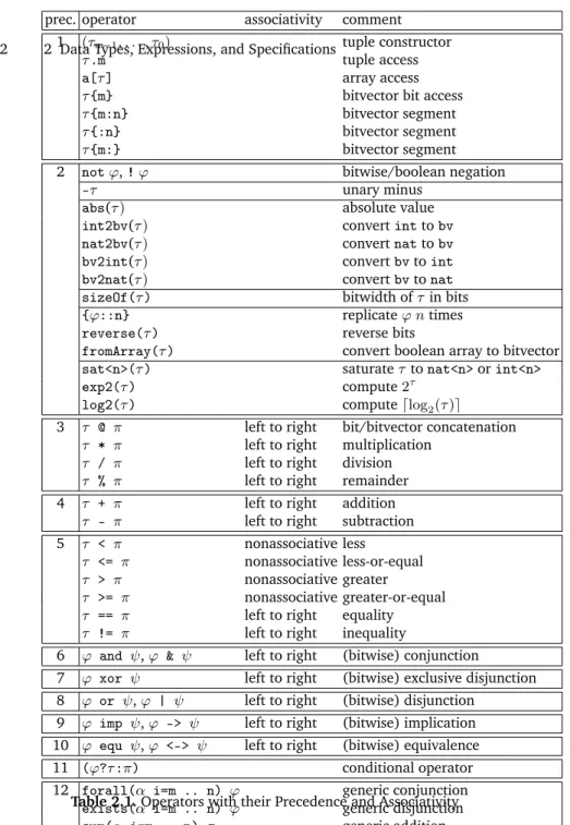
Table 2.1 lists all available operators together with their precedence (which is important to save delimiters for parsing) and associativity (for bi-nary operators only). Precedence 1 is the highest and 12 the lowest, so that a and b or c is a disjunction whose left hand argument is a conjunction. One has to use delimiters like ina and (b or c)to construct a conjunction whose right hand argument is a disjunction.
Associativities of binary operators is a further means to avoid ambigu-ity in expressions. As and is left-associative, the expressiona and b and c is parsed as (a and b) and c, so that delimiters are required to construct a and (b and c) if desired. We followed the definition of the C program-ming language in that we used the same syntax, precedences, and associa-tivities whenever possible. There are however minor differences: In contrast to the C programming language, comparison operators like<are not associa-tive in Quartz, since they can not be nested unlike in C. However, equality ==and inequality can be nested. For example,a == b == c will be read as (a == b) == cwhich implies thatcmust have typebool, and thataandb have the same type.
For boolean operators, one there is the alternative syntax!,&,|,->,^,<-> instead ofnot,and,or,imp,xor, andequ. Note that==and!=are equivalent to<->andxor, respectively. Nevertheless, we recommend the use of<->and xor, since these operators can also be bitwisely applied to bitvectors, which is not the case with==and!=(these return boolean values in this case).
Typing Rules
Table2.1presents the syntax of operators that includes the precedences and associativity rules. Clearly, not every expression that can be formed by these syntax rules is a legal expression, since expressions have to be additionally correctly typed. The type system used in Quartz can be summarized in a short hand notation and is shown in Figures2.1-2.3, whereτ : αmeans that the typeαcan be derived for expressionτ.
Figure2.1presents implicit and explicit type conversion rules. Note that the type of an expression is not uniquely determined, since the rules of Fig-ure2.1allow us to switch from one type to another one. However, there is always a minimal type with respect to the partial order relation of Defini-tion2.3, and this type is uniquely determined. We therefore distinguish be-tween a type of an expression or its minimal type. Rules (I.1)-(I.10) present the implicit type conversion rules that do not require operators and are used
22 2 Data Types, Expressions, and Specifications1 (τn−1, . . . , τ0) tuple constructor
τ.m tuple access
a[τ] array access
τ{m} bitvector bit access
τ{m:n} bitvector segment
τ{:n} bitvector segment
τ{m:} bitvector segment
2 notϕ,!ϕ bitwise/boolean negation
-τ unary minus
abs(τ) absolute value
int2bv(τ) convertinttobv
nat2bv(τ) convertnattobv
bv2int(τ) convertbvtoint
bv2nat(τ) convertbvtonat
sizeOf(τ) bitwidth ofτin bits
{ϕ::n} replicateϕ ntimes
reverse(τ) reverse bits
fromArray(τ) convert boolean array to bitvector
sat<n>(τ) saturateτtonat<n>orint<n>
exp2(τ) compute2τ
log2(τ) computedlog2(τ)e
3 τ @ π left to right bit/bitvector concatenation
τ * π left to right multiplication
τ / π left to right division
τ % π left to right remainder
4 τ + π left to right addition
τ - π left to right subtraction
5 τ < π nonassociative less
τ <= π nonassociative less-or-equal
τ > π nonassociative greater
τ >= π nonassociative greater-or-equal
τ == π left to right equality
τ != π left to right inequality
6 ϕ and ψ,ϕ & ψ left to right (bitwise) conjunction
7 ϕ xor ψ left to right (bitwise) exclusive disjunction 8 ϕ or ψ,ϕ | ψ left to right (bitwise) disjunction
9 ϕ imp ψ,ϕ -> ψ left to right (bitwise) implication 10 ϕ equ ψ,ϕ <-> ψ left to right (bitwise) equivalence
11 (ϕ?τ:π) conditional operator
12 forall(α i=m .. n) ϕ generic conjunction
exists(α i=m .. n) ϕ generic disjunction
sum(α i=m .. n) τ generic addition Table 2.1.Operators with their Precedence and Associativity
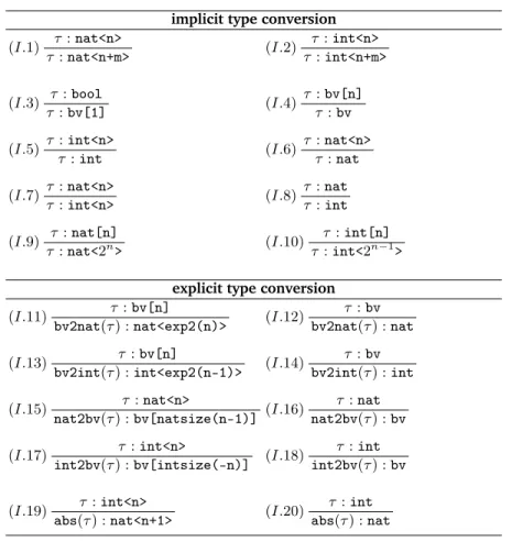
by the type checker itself whenever necessary. Without these rules, the min-imal type of an expression is derived, while the use of these rules switches to a supertype. In particular, rule (I.1) is the embedding ofnat<n>in the su-pertype nat<n+m>and rule (I.2) is the analogous rule for the types int<n> and nat<n+m>. In binary representations, these rules correspond with digit
implicit type conversion (I.1) τ:nat<n> τ:nat<n+m> (I.2) τ :int<n> τ :int<n+m> (I.3) τ :bool τ:bv[1] (I.4) τ :bv[n] τ:bv (I.5) τ:int<n> τ :int (I.6) τ :nat<n> τ:nat (I.7) τ:nat<n> τ:int<n> (I.8) τ :nat τ :int (I.9) τ:nat[n] τ:nat<2n> (I.10) τ :int[n] τ :int<2n−1>
explicit type conversion (I.11) τ:bv[n] bv2nat(τ) :nat<exp2(n)> (I.12) τ :bv bv2nat(τ) :nat (I.13) τ :bv[n] bv2int(τ) :int<exp2(n-1)> (I.14) τ :bv bv2int(τ) :int (I.15) τ:nat<n> nat2bv(τ) :bv[natsize(n-1)] (I.16) τ :nat nat2bv(τ) :bv (I.17) τ :int<n> int2bv(τ) :bv[intsize(-n)] (I.18) τ :int int2bv(τ) :bv (I.19) τ:int<n> abs(τ) :nat<n+1> (I.20) τ :int abs(τ) :nat
Fig. 2.1.Type System of Quartz (Part I)
extensions as explained in Lemma B.25. Rules (I.3) states that bool is also viewed as bv[1], and rules (I.4)-(I.6) state that the bounded types bv[n], nat<n>, andint<n>are included in the corresponding unbounded typesbv, nat, andint. Rules (I.9) and (I.10) introduce the shorthand notationnat[n], andint[n]to specify bounded numeric types via their binary bitwidths.
Rules (I.11)-(I.20) describe explicit type conversion rules, i.e., operators that are used to change a type of an expression with an according conver-sion function. Rules (I.11) and (I.12) convert bitvectors to natural numbers, where the bitvector is viewed as a radix-2 number. Similarly, rules (I.13) and (I.14) convert bitvectors to integers, where the bitvector is viewed as a 2-complement number. Note thatnbit radix-2 numbers encode the2nnumbers
(II.1) τn−1 :αn−1. . . τ0:α0 (τn−1, . . . , τ0) :αn−1 * . . . * α0
(II.2) τ :αn−1 * . . . * α0 π:nat<n>
τ.π:αJπKξ (II.3) τ:array(α,n) π:int<n>
τ[π] :α (II.4) τ :bv[n] π:bv[m] τ@π:bv[n+m] (II.5) τ:bv[n] π:int<n> τ{π}:bool (II.6) τ :bv[n] π1 :int<n> π2:int<n> τ{π1:π2}:bv[p1−p2+ 1] (II.7) τ:bv[n] π:int<n> τ{π:}:bv[p1+ 1] (II.8) τ :bv[n] π:int<n> τ{:π}:bv[n−p2]
(bitwise) boolean operators (same rules also for unboundedbv) (II.9) τ:bv[n] π:bv[n] τ & π:bv[n] (II.10) τ :bv[n] π:bv[n] τ | π:bv[n] (II.11) τ:bv[n] π:bv[n] τ -> π:bv[n] (II.12) τ :bv[n] π:bv[n] τ <-> π:bv[n] (II.13) τ:bv[n] π:bv[n] !τ :bv[n] (II.14) τ :bv[n] π:bv[n] τ xor π:bv[n]
arithmetic operators (same rules also for unbounded types) (II.15) τ:nat<m> π:nat<n>
τ + π:nat<m+n-1> (II.16)
τ :int<m> π:int<n>
τ + π:int<m+n>
(II.17) τ:nat<m> π:nat<n>
τ - π:nat<m> (II.18)
τ :int<m> π:int<n>
τ - π:int<m+n>
(II.19) τ :nat<m> π:nat<n>
τ * π:nat<(m-1)*(n-1)+1> (II.20)
τ :int<m> π:int<n>
τ * π:int<m*n+1>
(II.21) τ:nat<m> π:nat<n>
τ / π:nat<m> (II.22)
τ :int<m> π:int<n>
τ / π:int<m+1>
(II.23) τ:nat<m> π:nat<n>
τ % π:nat<n-1> (II.24) τ :int<m> π:int<n> τ % π:nat<n-1> (II.25) τ :nat<n> -τ:int<n> (II.26) τ:int<n> -τ :int<n+1> arithmetic relations (II.27) τ:int π:int
τ < π:bool> (II.28)
τ :int π:int
τ > π:bool>
(II.29) τ:int π:int
τ <= π:bool> (II.30)
τ :int π:int
τ >= π:bool>
(II.31) τ:int π:int
τ == π:bool> (II.32)
τ :bv[m] π:bv[n]
τ == π:bool>
(II.33) τ:int π:int
τ != π:bool> (II.34)
τ :bv[m] π:bv[n]
τ != π:bool>
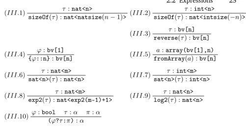
(III.1) τ :nat<n>
sizeOf(τ) :nat<natsize(n−1)> (III.2)
τ :int<n> sizeOf(τ) :nat<intsize(−n)> (III.3) τ:bv[n] reverse(τ) :bv[n] (III.4) ϕ:bv[1] {ϕ::n}:bv[n] (III.5) a:array(bv[1],n) fromArray(a) :bv[n] (III.6) τ:nat<m>
sat<n>(τ) :nat<n> (III.7)
τ :int<m> sat<n>(τ) :int<n>
(III.8) τ :nat<m>
exp2(τ) :nat<exp2(m-1)+1> (III.9)
τ :nat<n> log2(τ) :nat<n>
(III.10) ϕ:bool τ:α π:α
(ϕ?τ:π):α
Fig. 2.3.Type System of Quartz of (static) Expressions
inverse conversions are typed in rules (I.15)-(I.18), where natsize(n) and intsize(n)are defined below. Finally, rules (I.19) and (I.20) show how the absolute value function is used to convert signed to unsigned integers.
Definition 2.4 (Minimal Bitwidths). For every n ∈ N and everym ∈ Z, we
define the numbernatsize(n)∈Nandintsize(m)∈Nas follows: • natsize(n) :=
dlog2(n+ 1)e forn >0
1 forn= 0
• intsize(n) :=
1 +dlog2(n+ 1)e forn >0
1 forn= 0
1 +dlog2(−n)e forn <0
As shown in AppendixB,natsize(n)is the minimal number of bits required to represent the numbern∈Nin binary format, andintsize(n)is the minimal number of bits required to represent the numbern∈Zin 2-complement.
Rule (II.1) is the type rule of the tuple constructor that generates, e.g., from two expressionsτ andπthe pair(τ, π). Rule (II.2) is the type rule of the tuple selector operator that selects from a tuple like (τ, π)a component like (τ, π).1 =π.
Rule (II.3) refers to array access, where the expressiona[τ]is allowed to also have array type. Note however that except for array access there is no operator that would accept an expression of array type. Moreover, also the assignment statement is only allowed for atomic types. Note that the type int<n> is allowed for the index expression as will be discussed in the next section.
Rules (II.4)-(II-8) are type rules for bitvector expressions. Rule (II.4) de-scribes the construction of bitvectors by the concatenation operator. Rule (II.5) defines the access to a single bit of a bitvector expression. Rules (II.6)-(II.8) define the types of different versions of the slicing operator. Note that
the index expressions π, π1, and π2 are static expressions which is a major distinction to array accesses. Analogous to array accesses, we also allow the typeint<n>for the index expressions.
Rules (II.9)-(II.14) describe the type rules for the (bitwise) boolean op-erators. Note that due to rule (I.3) these operators can also be applied to arguments of typebool. Rules (II.15)-(II.26) are the type rules of the arith-metic operators that should be clear. The ranges of the used types are ob-tained by considering the minimal and maximal values or -1 (as in case of (II.11)). The rules (II.9)-(II.14) do also apply for unbounded types. The rules for arithmetic relations (II.27)-(II.34) are only stated for typeint. However, asnat<m>,nat, andint<m>are subtypes ofint, we can use these rules also for these subtypes in any combination. Note that the equality of bitvectors accepts argument types of different bitwidths (the result is false for different bitwidth).
Rules (III.1) and (III.2) describe possible uses of thesizeOfoperator that can compute the minimal numbers of bits required to implement expressions of typesnat<n> andint<m>as radix-2 and 2-complement numbers, respec-tively. (III.3) is the typing of thereverseoperator. Rule (III.4) describes the bit-iterator that generates n copies of a boolean expression in a bitvector. Rule (III.5) explains how the fromArrayoperator converts a boolean array to a bitvector. Note that the inverse operation can be easily obtained by a generic sequence of assignments as explained in the section on statements. Rules (III.6) and (III.7) are the type rules for the satoperator that imple-ments saturated arithmetics as explained in the next section. The remaining rules should be clear.
Note that we do not list type rules for generic conjunction, generic disjunc-tion, and generic sums, since these are viewed as abbreviations of expressions whose type rules have already been given.
Semantics
Having explained the syntax and the type inference rules of expressions, it remains to formally define the meaning of expressions. In general, we define the semanticsJτKξ of an expression τ with respect to a variable assignment ξ and assume that the variable assignmentξ is type consistent, i.e., that for every variable x, the value ξ(x)belongs to the semantics of the type of x. This holds also for the semanticsJτKξ of an expressionτ, i.e., alsoJτKξ is an
element of the set of values that is associated with the type ofτ.
In general, the semanticsJτKξ of an expression τ depends onξ, so that
whenever the variable assignment changes, also the semanticsJτKξ may be changed. Therefore, the semantics of an expression is rather a function that depends on the expression and on a variable assignment. This is in particular convenient to describe the change of the semantics of an expression during the execution of the program where the values of the variables are changed.