The Impact of Railway Stations on Residential
and Commercial Property Value: A Meta-analysis
Ghebreegziabiher Debrezion&Eric Pels&
Piet Rietveld
Published online: 19 June 2007
#Springer Science + Business Media, LLC 2007
Abstract Railway stations function as nodes in transport networks and places in an urban environment. They have accessibility and environmental impacts, which contribute to property value. The literature on the effects of railway stations on property value is mixed in its finding in respect to the impact magnitude and direction, ranging from a negative to an insignificant or a positive impact. This paper attempts to explain the variation in the findings by meta-analytical procedures. Generally the variations are attributed to the nature of data, particular spatial characteristics, temporal effects and methodology. Railway station proximity is addressed from two spatial considerations: a local station effect measuring the effect for properties with in 1/4 mile range and a global station effect measuring the effect of coming 250 m closer to the station. We find that the effect of railway stations on commercial property value mainly takes place at short distances. Commercial properties within 1/4 mile rang are 12.2% more expensive than residential properties. Where the price gap between the railway station zone and the rest is about 4.2% for the average residence, it is about 16.4% for the average commercial property. At longer distances the effect on residential property values dominate. We find that for every 250 m a residence is located closer to a station its price is 2.3% higher than commercial properties. Commuter railway stations have a consistently higher positive impact on the property value compared to light and heavy railway/Metro stations. The inclusion of other accessibility variables (such as highways) in the models reduces the level of reported railway station impact.
Keywords Property value . Railway station . Accessibility . Light railways . Heavy railway/metro . Commuter railway . Meta-analysis
DOI 10.1007/s11146-007-9032-z
G. Debrezion (*)
:
E. Pels:
P. RietveldFree University Amsterdam, Department of Spatial Economics, De Boelelaan 1105, 1081 HV Amsterdam, The Netherlands
e-mail: gdebrezion@feweb.vu.nl E. Pels
e-mail: apels@feweb.vu.nl P. Rietveld
Introduction
Location choice is a frequently discussed topic in urban economics. These discussions can be normative or descriptive in nature. Thus, in the literature we find two approaches to urban location analysis. The first set of studies addresses the issue of optimal location conditional to a given set of constraints (Fujita1989). The second set of studies is devoted to explaining the character (value) of a property at a given location. However, the issue of identifying the factors that affect property values is common to both sets of approaches. Our discussion will basically address studies of the latter category, focusing on the relationship of property values and railway stations.
In the context of this paper, property means an estate ranging from a vacant piece of land to an area occupied by all sorts of buildings: residential, commercial, industrial etc. (Brigham 1965). Several studies have tried to address the discussions on property value. There is a general consensus among most authors in categorizing the factors affecting property values as physical, environmental and accessibility factors (Fujita 1989; Bowes and Ihlanfeldt 2001). However, some authors have included historical factors and land use patterns into their analysis (Brigham1965). Numerous detailed lists of features can be identified within each of these categories. As to the relevance of the factors to the analysis, the detailed list can differ from one place to another and thereby from study to study.
Accessibility as provided by different modes of transportation and railway in particular, as a factor affecting property value, has also received some attention in the literature. The most common way of addressing the railway accessibility was by including the proximity factor in the analysis. This paper discusses the results of studies which have addressed the effect of railway stations on property value. The paper has two parts, a qualitative review and a quantitative analysis. The first part of the paper surveys studies on the effect of railway station proximity on property value. In the second part, meta analytical analysis is applied to systematically explain the variation in the findings on the impact of railway station proximity on property value across studies. Thus, in subsequent sections, we discuss the theoretical foundation of the studies, presenting and comparing the empirical results of the various studies conducted. In addition to the reviewing of studies conducted in the area, we make a quantitative analysis of the results of the studies, using meta-analysis to explain the differences in the results.
Literature Review: Theories and Findings
Most land value theories have their root in the work of Von Thünen (1863), who tried to explain variations in farmland values. According to Von Thünen, accessibility to the market place explains the value difference of farmlands for agricultural lands having similar fertility. In subsequent studies, economists like Alonso and Muth refined this line of reasoning into a bid-rent analysis (Alonso1964; Muth1969). The basic idea behind the bid-rent model is that every agent is prepared to pay a certain amount of money, depending on the location of the land. This leads to a rent gradient that declines with distance from the central business district (CBD) for sites that
yield equal utility. Thus, far in the analyses, the dominant factor explaining the difference between land (property) values was the accessibility as measured by the distance to the CBD and the associated transportation costs. The physical characteristics of the land (fertility in the case of Thünen) were assumed given.
Thus, the basic theory on real estate prices can be put forward as follows: as a location becomes more attractive, due to certain characteristics, demand increases and thus the bidding process pushes prices up. In most cases CBDs are the centres of many activities. Therefore, closeness to the CBD is considered as an attractive quality that increases property prices. However, investments in transport infrastructure reduce this demand friction around the CBD to some degree (Fejarang 1994) by attracting households to settle around the stations. Properties close to the investment area (railway stations) enjoy benefits from transportation time and cost saving as a result of the investment. It may be expected that a price curve will have a negative slope; when we move away from the station, prices decrease.
The introduction of the hedonic pricing methodology (Rosen1974) led to an easier way of attributing effects on property value to features comprising the properties. Thus, we observe the integration of physical, accessibility and environmental characteristics of properties in models trying to explain the difference in property values. Accessibility remains an important feature for urban properties. However, earlier attempts to account for it by transportation cost have been narrow. Attempts have been made to introduce a broader concept of accessibility as to include all features that contribute to the potential of opportunities of a location for interaction (Hansen 1959; Martellato et al. 1998). Though a comprehensive definition of the concept of accessibility is available, in practical applications the lack of data and appropriate measuring techniques usually implied that simple measures are used. Thus, in the literature we see a focus on some factors only, especially a CBD oriented interaction related to employment and shopping. In most property value studies, the other trip purposes are missing from the model.
The main focus in this paper is the analysis on the impact of railway accessibility as attributed by proximity to railway stations. However, it is important to realize that accessibility can also be provided by other modes of transport. As Voith (1993) has pointed out, highway accessibility is an important competitor to rail accessibility.
‘The presence of other facilities that increase accessibility like highways, sewer services and other facilities influence the impact area in the same fashion.’ The benefits of these facilities and services are also capitalised into urban property values (Damm et al. 1980). Thus, to single out the effect of railway accessibility, other competing modes of accessibility need to be included along with it.
The motivations for the studies on the impact of railway accessibility are diverse. The larger part of the literature on railway focuses on it as a feasible solution to the rising congestion posed by automobile traffic and urban sprawls. Railway investment is expected to support a more compact urban structure and therefore it serves the urban planning purpose (Goldberg 1981). Apart from reasons of showing that railway investments do result in compact urbanisation, most studies in the area were conducted to provide evidence for the implementation of value capture schemes for financing rail investments (Cervero and Susantono1999). This was based on the assertion that the value of proximity to accessibility points is capitalised on the value of properties around these stations.
In general the empirical studies conducted in this area, on the impact of railway accessibility on property values, are diverse in methodology and focus. Although the functional forms can differ from study to study, the most common methodology encountered in the literature is hedonic pricing. However, no consistent relationship between proximity to railway stations and property values is recorded. Furthermore, the magnitudes of these effects can be minor or major. In one of the earliest studies, Dewees (1976) analysed the relationship between travel costs by railway and residential property values. Dewees found that a subway station increases the site rent perpendicular to the facility within a 1/3 mile to the station. Similar findings confirmed that the distance of a plot of land from the nearest station has a statistically significant effect on the property value of the land (Damm et al.1980). Consistent with these conclusions, Grass (1992) later found a direct relationship between the distance of the newly opened metro and residential property values. Some of the extensively studied metro stations in the U.S., though ranging from small to modest impact, show that properties close to the station have a higher value than properties farther away (Giuliano 1986; Bajic 1983; Voith 1991). However, there are also studies, which have found insignificant effects (Lee1973; Gatzlaff and Smith 1993). On the other hand, contrary to the general assumption, Dornbusch (1975), Burkhart (1976) and Landis et al. (1995) traced a negative effect of station proximity. Evidence from other studies indicates little impact in the absence of favourable factors (Gordon and Richardson 1989; Giuliano 1986). For detailed documentation of the findings, we refer to (Vessali1996; Smith2001; NEORail II
2001; Hack 2002; RICS, Policy Unit 2002). In general, some studies indicate a decline in the historical impact of railway stations on property values. This was attributed to improvements in accessibility, advances in telecommunications, computer networks, and other areas of technology that were said to make companies
“footloose”in their location choices (Gatzlaff and Smith1993).
Our main aim in this paper is to systematically analyse the variation in the findings of the studies discussed above. We use meta-analysis to provide a statistical analysis of the variations in the study findings. The impact of a railway station on the property values depends on several factors. First, railway stations differ from each other in terms of levels of service provided in terms of frequency, network connectivity, service coverage etc. Thus, it is natural to see stations with differing impact levels on the value of surrounding properties. Commuter railways have a relatively high impact on property value (Cervero and Duncan2001; NEORail II
2001; Cervero1984). Railway stations can differ in the level and quality of facilities they have. Stations with a higher level and quality of facilities are expected to have greater impact on the surrounding properties. The presence and number of parking lots is one of the many station facilities that got attention in this area. Bowes and Ihlanfeldt (2001) found that stations with parking facilities have a higher positive impact on property values. In addition, the impact a railway station produces depends on its proximity to the CBD. Stations, which lie close to the CBD, produce greater positive impact on property value (Bowes and Ihlanfeldt2001). In addition Gatzlaff and Smith (1993) claim that the variation in the findings of the empirical work is attributed to local factors in each city.
Second, railway stations affect residential and commercial properties differently. Most studies treated the effect of railways on the different property types separately.
That allows us somehow to explain the difference of railway effects on different property types. Generally it has been shown that the impact of railway stations is greater within short distance of the stations on commercial properties compared to residential ones. The larger part of the empirical literature on property value focuses on residential properties rather than commercial properties. Generally, it is claimed that the range of the impact area of railway stations is larger for residential properties, whereas the impact of a railway station on commercial properties is limited to immediately adjacent areas. In addition, there are claims that railway stations have a higher effect on commercial than on residential properties (Weinstein and Clower 1999; Cervero and Duncan 2001). This finding is in line with the assertion that railway stations—as focal, gathering points—attract commercial activities, which increase commercial property values. However, contrary to this assertion, Landis et al. (1995) determined a negative effect on commercial property values.
Third the impact of railway station on property value depends on demographic factors. Income and social (racial) divisions are common. Proximity to a railway station is of higher value to low-income residential neighbourhoods than to high-income residential neighbourhoods (Nelson1998; Bowes and Ihlanfeldt2001). The reason is that low-income residents tend to rely on public transit and thus attach higher value to living close to the station. Because of the fact that reaching the railway station mostly depends on slow modes (waking and bicycle) the immediate locations are expected to have higher effects than locations further away. On the other hand the high population movement in the immediate location gives rise to the development of retail activities which leads to premiums on value of commercial properties, but at the same time it may attract criminality (Bowes and Ihlanfeldt2001). Bowes and Ihlanfeldt (2001) outlined that a significant relation was observed between stations and crime rates. In their model, the immediate neighbourhood is affected negatively by the station. Thus, the most immediate properties (within a quarter of a mile of the station) were found to have an 18.7% lower value. Properties that are situated between one and 3 miles from the station, however, are more valuable than those further away. Though this study provides an important contribution, unexplained variations still remain.
Meta-analysis of the Studies
In the previous section we briefly reviewed empirical work on the effects of station proximity on property value. Other reviews can be found in Vessali (1996), Smith2001, NEORail II (2001), CIP Annual Conference (2002) and RICS, Policy Unit (2002). These studies also summarized empirical work in this area, but did not look for a systematic explanation of the variation in the findings. Our study not only summarizes earlier work, but also looks for a systematic explanation of differences in the results. Meta-analysis serves as an important tool for this purpose (Smith and Hang1995; Cook et al.1992). It provides statistical synthesis for empirical research focused on a common research question. It includes variables that represent study settings that are expected to explain the variation in the findings of the studies. In this case, all the reviewed studies focus on the impact of railway station proximity on property value. For the comparison of results to be meaningful, it is required that the studies have a comparable unit for the effect. However, in the studies which address the relationship
between proximity to a railway station and property value we encounter different measurement units, although they aim at measuring similar effects. Thus, it is important that the findings are converted in to the same measurement unit.
In this study we apply a meta-regression model. The effect sizes of proximity to the railway station on property value found by the different studies are the dependent variables, whereas the implicit or explicit characteristics of the underlying studies make up the dependent variables. A basic meta-analysis equation can be given as follows (Florax et al.2002).
Y ¼f Pð ;X;R;T;LÞ þ" ð1Þ where
Y the variable under study P set of causes of the out comeY
X characteristics of the set of objects under examination affected byPin order to determine the outcomeY
R characteristics of research method T time period covered by the study L the location of each study conducted
ɛ the error term Model Specification
Meta analysis models try to explain the difference in study findings by difference in study characteristics and other variables, for instance time and geographical effects. Thus, generally they belong to the family of hedonic pricing models. The logical order is first to identify the characteristics of the underlying studies that could explain the variations in effect sizes. The underlying studies usually include the proximity of the property to the station. However, we observe that not all studies use the same set of (explanatory) variables. The studies also differ in methodology. A railway station variable is mostly treated as a sole indicator of accessibility of a certain area. However, other modes serve the same purpose; for example, highway/ freeway presence in the area under consideration. Although for our purpose it is important to note that they both have an effect on property values one can expect that these modes“interact”in a complementary (one can take a car to the railway station and then take the train) or competitive way (use car or train).
The underlying empirical studies employ different specifications, namely linear, semi logarithmic and log linear. In some studies the analyses are non-parametric in nature. Different specifications may also lead to different outcomes. In our analysis we further include type of railway station (light rail, heavy rail/Metro, commuter rail and Bus rapid transit), type of property (commercial, residential). We drop the location feature of the studies from our model because all the studies that are used in our final analysis were done in the US. We also examine whether the underlying study includes variables for the features of the properties and demographic features. All studies include features of the property in their analysis. Thus, our analysis includes six categories of variables to explain the difference in the findings of the impact of railway station proximity on property values. To account for the variation
we specify a standard hedonic model using a simple linear regression specification given by Eq.2below.
Y ¼α0þblPþβ2Sþβ3Mþb4ACCESSþb5DMþb6Tþ" ð2Þ
Dependent variable Yis the effect size for the impact of railway station proximity on property value (rent) in percentages.
Explanatory variables P is a dummy variable that takes on the value 1 when commercial properties are analyzed (reference group is taken to be residential properties).Sis a vector of dummy variables for the station type (heavy rail/ Metro, commuter rail, Bus rapid transit; light rail is the reference group).Mis a vector of dummy variables for the model type (semi log, double log, non parametric; linear is the reference group). ACCESS is a dummy variable indicating the inclusion of other means of access to the area in the underlying study (usually highways and/or freeways). DM is a dummy variable indicating the presence of a demographic variable in the underlying study (usually income or racial composition of city quarters).T is a dummy for time trend (assume 1 for study data after 1990, study data before 1990 is taken as a reference group).
Some of these variables were used in the models of the underlying studies. Because most variables in the meta-analysis are dummy variables, the estimated coefficients represent the percentage contribution of each attribute on property value in comparison to the reference groups.
Data and Methodology
The database for the analysis of this paper is a pool of studies on the impact of railway station proximity on property value. A wide range of studies is covered. A total of 73 estimation results were obtained from the underlying studies. All these studies try to quantify the impact of proximity to a railway station on property values. Different specifications in the same underlying study are treated as separate observations. Thus, the total number of underlying studies is lower than the number of observations in our meta-analysis. However, due to the incompleteness of some of the studies with respect to the requirements of this study, we had to exclude certain observations. Our final estimation is based on 57 observations.
Variation in the Presentation of the Findings
The dependent variable in our meta-analysis is expressed as the percentage change in property value per some distance measure to the station. The underlying studies are quite diverse in the way the impact of railway station proximity is reported, including pure monetary effects, percentage effects and elasticity measures. However, the larger part of these studies reports the percentage increase or decrease in property value for a certain distance. In addition to the diversity of measurements,
the studies also use a variety of methodologies. We summarize them in two categories; which are discussed next.
I. Studies using parametric estimation methods
These studies use econometric methods to estimate the impact of railway station proximity on property value. Linear, semi log and log linear (also called double log) specifications are common. Two categories of railway station proximity measure-ment were encountered.
1. Station proximity as a continuous measure
These studies consider the proximity to a railway station as a continuous variable. The variable can be measured in distance, time (walking time) or monetary savings
(Dewees 1976; Nelson 1992; Benjamin and Sirmans 1996; Lewis-Workman and
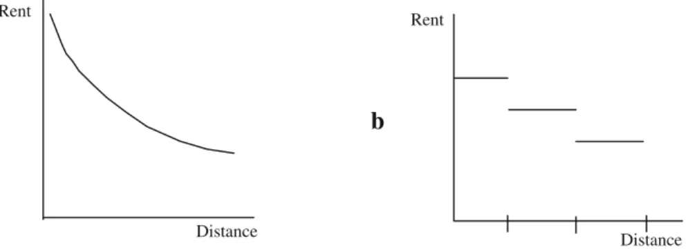
Brod1997; Chen et al. 1998; Gatzlaff and Smith 1993). The results are given in monetary units (as in linear models) or in percentage units (as in semi log and log linear models). The results of the semi log models are in line with the dependent variable in our meta-analysis. Therefore, the monetary changes and elasticities have to be transformed into a percentage change per distance using the average property value and average distance data reported in each underlying study. Coefficients of semi log and double log specifications represent incomparable measures. To bring them into comparable units we divided the elasticity by the average distance of the impact area. The rent curves can have structures similar to (a) in Fig.1(Table 1).
2. Station proximity as a distance category measures:
These studies treat the proximity variable as a discrete variable (represented by a dummy). The area under consideration is segmented into two or more parts, where
the outer segment is treated as the reference (McDonald and Osuji1995; Fejarang
1994; Dueker and Bianco1999; Weinstein and Clower 1999; Voith1993; Armstrong
1994; Grass1992; Bowes and Ihlanfeldt2001; Cervero and Duncan2001,2002a,b; Weinberger2001). Sample of presentation of effects of this type are given in Table2. The rent curve for these types can be given by (b) in Fig.1.
II. Non-parametric measures:
These studies do not use econometric methods to estimate the effect of railway stations on property values. They can measure the proximity variable in continuous
Rent
Distance
Rent
Distance
a
b
Fig. 1 Structure of rent curves; distance from the station as a continuous measure (a) and as category measures (b)
or discrete terms. The common feature of these studies is that the difference in property value is implicitly attributed to the railway station effect only. Some examples of this sort are given in Table3.
The Dependent Variable in the Meta-analysis
For meta-analysis it is essential that the dependent variable is measured in comparable units. Due to the diverse ways of presenting the effect sizes, a matching process was necessary to transform them in to effect sizes of the same measurement unit. For the purpose of our analysis, two proximity measures considerations are selected: a stepwise treatment and continuous treatment on proximity. From the stand point of the stepwise treatment of distance, the effect of railway station proximity on values of properties located within 1/4 mile of the station effect was prominent. Thus, we prepared the effect of railway on the property value for properties located within this range compared to the properties out of this range. In addition, an effect size for the continuous distance treatment was prepared. For this consideration the effect sizes of railway station proximity impact on property value for every 250 m closer to the station are prepared.
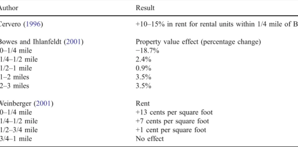
Table 2 Sample of railway station effects on property value based on distance category measures
Author Result
Cervero (1996) +10–15% in rent for rental units within 1/4 mile of BART Bowes and Ihlanfeldt (2001) Property value effect (percentage change)
0–1/4 mile −18.7% 1/4–1/2 mile 2.4% 1/2–1 mile 0.9% 1–2 miles 3.5% 2–3 miles 3.5% Weinberger (2001) Rent
0–1/4 mile +13 cents per square foot
1/4–1/2 mile +7 cents per square foot
1/2–3/4 mile +1 cent per square foot
3/4–1 mile No effect
Table 1 Sample of railway station effects on property value based on continuous proximity measures Author Railway station impact on property value
Dewees (1976) $2,370 premium per hour of travel time saved for sites within 20 min travel time (e.g. 1/3 mile walk)
Nelson (1992) $1.05 per feet distance to the station. Premium on property value in low-income areas;
$.96 per feet distance to the station.
Allen et al. (1986) $443 premium on property value for every dollar saved in daily commute costs (average >$4,500 per house; 7.3% of mean sales price)
Lewis-Workman and Brod (1997)
Elasticity of 0.22 with regard to property value and distance Benjamin and Sirmans
(1996)
Rent decreased by 2.4 to 2.6% for each 1/10 mile distance from the metro station
Due to the large differences between the underlying studies in reporting the finding some conversion mechanism is required. We mention three elements of this mechanism:
1. We consider railway station impacts up to a maximum distance of 2 miles, unless otherwise indicated.
2. The properties under study are evenly distributed in concentric circles around the railway stations. Thus, due to the fact that larger circles lead to an area enlargement, the average distance to the station for each segment is given bya+ 2/3*(b−a), whereais the distance the border of the inner concentric circle to the station, and bis the distance between the border of the outer segment and the railway station. For the station itself we havea=b=0.
3. The impact of a station in the same segment in a circle is uniform.
For studies that provide the impact for several segments, the continuous railway station impact (see for example Table2) is estimated by the approach outlined in
Appendix. However, for studies that looked at one (immediate) segment, as compared to the outer segment, we have estimated the continuous station effect per distance by point estimation (under the above assumptions). The type of model used to determine the effect can actually influence the effect (compare e.g. point elasticity estimates to interval estimates). Although most studies were parametric, a few studies used a non-parametric model, as discussed above. We adopt a unit of measurement equal to 250 m. Thus, the dependent variable in the meta-analysis is the percentage change in property value (rent) for every 250 m coming closer to the railway station. In addition we have prepared the effect of the railway station on the immediate segment (within a quarter mile of the station). Therefore, our estimation is based on these two data sets. Independent Variables
The impact of railway station proximity on station on property value as reported in the underlying studies can be affected by several factors. The type of property value under study may be important, because commercial and residential properties may be affected differently. Different types of railway stations may have different impacts because the frequency of service or the service coverage may be different, etc. Four types of rail transit services are identified: light, heavy, commuter and rapid bus transits. Three types of parametric models were encountered: linear, semi-log and log
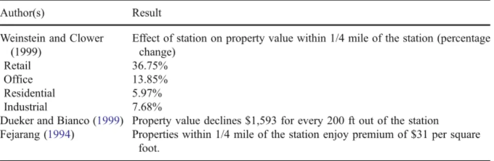
Table 3 Sample of results presentation for non-parametric cases
Author(s) Result
Weinstein and Clower (1999)
Effect of station on property value within 1/4 mile of the station (percentage change)
Retail 36.75%
Office 13.85%
Residential 5.97%
Industrial 7.68%
Dueker and Bianco (1999) Property value declines $1,593 for every 200 ft out of the station Fejarang (1994) Properties within 1/4 mile of the station enjoy premium of $31 per square
linear. Temporal effect is represented by dividing the data in two categories: data before 1990 and data after 1990. We also included a variable for the presence of other accessibility variables (highways and freeways are of interest here), and demographic features in the underlying studies, as discussed above. As shown in Table4, these considerations lead to six categories of dependent variables in our meta-analysis.
Descriptive Statistics
Table 5 presents the descriptive statistics of the dependent variable. Overall characteristics and characteristics per group (defined by the independent variables) of the dependent variable are given. The overall mean impact of a railway station on property value for properties that lay within 1/4 mile of the station compared to the value of properties laying beyond this range is 8.60%. The range of the property value effect is considerable: −61.90 to 145%. Concerning the continuous distance measure, the impact of a station on property value (rent) for every 250 m closer to the station is 2.61%. The t able shows that the range is considerable; it varies from
−12.84 to +38.70%. In computing the means no weighting is applied.
From Table5 we also learn that railway stations have a higher average effect on commercial properties compared to residential properties. However, the corresponding standard deviations are quite high. Commuter railway stations have higher impact on property values than the other three types of railway stations. Contrary to the literature assertion that railway stations have lower impact on multi family or condominium properties, as compared to single-family properties, the table indicates higher impact on single-family properties (Cervero1997; Cervero and Duncan 2002a,b), although the differences are not significant.
Table 4 Independent variables
Variable Description Type
Type of property (P)
RESIDENTIAL Residential property Dummy
COMMERCIAL Commercial Property Dummy
Type of station (S)
LRT Light rail transit station Dummy
HRT Heavy (rapid) rail transit station/Metro Dummy
COMMUTER Commuter rail transit station Dummy
BRT Rapid bus transit station Dummy
Type of underlying model (M)
LINEAR Model with linear specification Dummy
SEMI LOG Model with semi log specification Dummy
LOG LINEAR Model with log linear specification Dummy
Inclusion of accessibility variable(s) in the underlying model
ACCESSIBILITY (ACCESS) Dummy
Inclusion of demographic variable(s) in the underlying model: income, racial composition of city quarters
DEMOGRAPHIC (DM) Dummy
Time of data (T)
TIME Before 1990 Dummy
The table also gives some simple comparison tests of the means for each of the categories. Thettest statistic in the table is a group-wise mean equality test. In each category the equality test is done against the reference group in each category. The null and the alternative hypotheses of the test are given as follows. H0:
Mean ESjrefð Þ Mean ESjð jÞ ¼0 andHa: Mean ESjrefð Þ Mean ESjð jÞ 6¼0, where ES is the effect size of the studies,jis an identifier of a group in the same category as the reference (ref). For instance, for the category‘type of railway station’ light rail transit stations are the reference, whereas the other type of stations are compared to this. The test is performed under the assumption that population variance is the unique. The ttest statistic is given by:
T¼ ffiffiffiffiffiffiffiffiffiffiffiffiffiffiffiffiffiffiffiffiffiffiffiffiffiffiffiffiffiffiffiffiffiffiffiffiffiffiffiffiffiffiffiffiffiffiffiffiffiffiffiffiESref ESj nrefþnj nref:nj nref1 ð Þ:s2 refþðnj1Þ:s2j nrefþnj2 r ð3Þ
Table 5 Descriptive summary of railway station proximity impact on property value (measured in relative change)
Effect within 1/4 mile Effect per 250 m
N Min Mean Max SD ttest N Min Mean Max SD ttest
Over all 55 −0.619 0.081 1.452 0.263 57 −0.128 0.026 0.387 0.065 Property Type Residential 42 −0.193 0.046 0.429 0.118 44 −0.038 0.019 0.134 0.035 Commercial 13 −0.619 0.191 1.452 0.496 −1.773 13 −0.128 0.048 0.387 0.122 −1.428 Residential Properties Single familya 29 −0.187 0.048 0.370 0.098 31 −0.031 0.024 0.134 0.036 Condominium 6 −0.193 0.043 0.429 0.209 0.093 6 −0.038 0.008 0.084 0.041 0.963 Multi family 7 −0.086 0.040 0.291 0.121 0.196 7 −0.021 0.005 0.039 0.019 1.338 Type of railway stations LRTa 16 −0.072 0.071 0.302 0.093 18 −0.014 0.027 0.134 0.040 HRT 20 −0.619 0.021 0.370 0.199 0.933 20 −0.128 0.009 0.099 0.043 1.292 CRT 15 −0.270 0.187 1.452 0.425 −1.093 15 −0.056 0.053 0.387 0.105 −0.977 BRT 4 −0.149 0.017 0.200 0.147 0.942 4 −0.031 0.003 0.042 0.030 1.104 Model Lineara 43 −0.619 0.079 1.452 0.291 45 −0.128 0.023 0.387 0.071 Semi log 8 −0.187 0.085 0.370 0.157 −0.049 8 −0.006 0.037 0.099 0.040 −0.543 Log linear 4 0.050 0.085 0.137 0.040 −0.037 4 0.016 0.034 0.046 0.014 −0.356 No accessibilitya 12 0.005 0.127 0.370 0.109 13 0.002 0.049 0.134 0.039 Accessibility 43 −0.619 0.067 1.452 0.292 0.695 44 −0.128 0.019 0.387 0.070 1.485 No demographica 16 0.005 0.110 0.370 0.098 17 0.002 0.043 0.134 0.036 Demographic 39 −0.619 0.069 1.452 0.307 0.526 40 −0.128 0.019 0.387 0.073 1.277 Time Up to 1990a 13 0.005 0.095 0.370 0.097 14 0.002 0.045 0.134 0.035 After 1990 42 −0.619 0.076 1.452 0.297 0.226 43 −0.128 0.019 0.387 0.071 1.308 aReference group in the category
Random Effect Meta-regression Model
Meta analysis tries to explain variation in effect sizes by means of determinants as incorporated in Eq.2. In the literature, meta-regression is used from four different approaches: fixed effects, random effects, control rate, and Bayesian hierarchical modelling (Morton et al.2004). Fixed effect models assume that these estimates are random draws of one true value. The effect sizes included in the meta analysis represent the estimates of the true value for the study with some degree of imprecision. Thus, the variance in the meta analysis only comes from sampling error. However, substantial heterogeneity among the estimates can be an indication that the true effect value in the estimates is not unique. In such a situation Higgins and Thompson (2004) have indicated that fixed effect meta-regression models suffer from false positive results compared to the conventional regression model. The use of random effect models is believed to reduce spurious findings. In our case the standard Q statistics for the homogeneity test shows that the effect sizes of railway station proximity on property value show substantial heterogeneity1. This justifies the use of a random effects model for the meta analytical procedure. The random effects model assumes that the variance associated with each effect size has two components: the within study variance and the between studies variance.
In this paper we apply the random effect meta-regression model to explain the variation in the effect sizes of railway station proximity effect on property values. The variance of the effect size in this modelling approach is the sum of the two variance components, namely the within study variance σ2i and the between studies variance (τ2) components. Thus, the weight for each of the effect sizes is the reciprocal of this total variance wi¼1
σ2
i þτ2
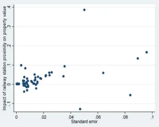
. The estimation procedure proceeds in two stages. First, the between studies variation measure (τ2) is determined. Second, using the updated weight considering the within study and between studies variation, the regression analysis is performed; the regression equation estimated in this paper is given in Eq.2. The Stata based meta-regression routine (metareg) is used to run the estimation. An important feature of the random effect meta-regression is that R-square is not reported; instead theτ2is reported. In Figs.2and3the effect sizes used in our analysis are plotted against the corresponding standard errors of the effect sizes. Both graphs show a similar pattern, although the scale is difference due to the different distance measures used.
Estimation Results
To explain the variation in the findings of the railway station proximity effect on property value by various study characteristics, we performed two estimations. As indicated in Section 3.2, the first estimation explains the impact of station proximity on the value (rent) of properties located within 1/4 mile (402 m) of the station. The
1
The homogeneity test’s Q statistics is given byQ¼ PwiESi2
ðPwiESiÞ2.Pwiwherewiis the weight of the effect size (ES) of studyigiven by the inverse of the variance.Qis chi-square distribution. For the data in the analysisQ=1,212, where the critical value for 5% and 56 degrees of freedom is 74.5. This indicates the effect sizes have substantial heterogeneity. This calls for a random effect model of estimation.
impact is measured as the relative change in property value. The second estimation explains the impact of station proximity on property value (rent) for every 250 m distance closer to the station. The explanatory variables for the two estimations are given in Table4. The outputs of the random effect meta-regression model based on 55 effect sizes are given below.
1. Local effect of railway proximity:
In this case the dependent variable is the effect of railway station proximity on properties lying within the 1/4 mile distance from the station, compared to properties located outside this range. This measures the most localized impact of railway Fig. 2 Plot of the railway station proximity effect for properties within 1/4 mile of the station against the standard error of the estimates
Fig. 3 Plot of the railway station proximity effect for every 250 m coming closer against the standard error of the estimates
station accessibility on property value. The distance category is common to many studies. In addition, this range represents locations within walking distance. The random effect estimation results for this specification are given in Table6.
In Table6we see theτ2is greater than 0 (which would be the outcome in the case the fixed effect assumption would hold). This shows that there is substantial variation between the effect sizes (ES) of the studies. This confirms the justification for the use of a random effect model. Railway station proximity has a higher effect on commercial property compared to residential properties. The gap between the price within the 1/4 mile zone and the remaining part of the city is larger for commercial property than it is for residential property: to be more precise: it is 12% larger. Table5shows that where the price gap between the railway station zone and the rest is about 4.2% for the average residence, it is about 16.4% for the average commercial property.
The coefficients for heavy and commuter rail transit are positive, indicating that the effects of heavy and commuter rail transit on property value are greater than light rail transit (the base line in the estimation). Heavy railway transit stations have a 0.9% higher effect on property value compared to the effect of light rail transit stations. However, the significance level for this variable is low. On the other hand, a commuter rail transit station has a significantly higher effect on property value compared to light rail transit stations. It has an effect as big as 14.1% higher than the effect of light rail transit stations. This finding is consistent with the a priori
expectation, and reflects the fact that commuter railways usually have wider service coverage (i.e. a larger catchment area).
The inclusion of other accessibility factors (highway, freeway) in the underlying studies significantly reduces the level of the reported station impact on property values (the reference group is the“no alternative accessibility variable in underlying study”). This shows that highways and freeways are also important determinants of property value (rent), next to railway station proximity. When both are included in the models (railway station and other modes) the effect on property value is“shared” between the two different modes. Models with highway accessibility on average
Table 6 Effect of railway on property values within 1/4 mile compared with other locations
Variable Coefficient Standard error z-value p-value
Constant 0.087 0.071 1.240 0.215
Commercial property 0.122 0.063 1.950 0.051*
Heavy rail transit (HRT) 0.009 0.051 0.180 0.857
Commuter rail transit (CRT) 0.141 0.063 2.260 0.024**
Bus rapid transit (BRT) −0.015 0.080 −0.180 0.856
Semi log specification (SEMILOG) −0.005 0.070 −0.080 0.940
Log linear specification (LOGLINEAR) −0.005 0.095 −0.050 0.956
Accessibility variables −0.187 0.094 −2.000 0.046**
Demographic variables 0.055 0.091 0.600 0.545
Time of data after 1990 0.029 0.061 0.480 0.633
No of studies=55
τ2 estimate=0.0153 *Significant at 10% **Significant at 5%
report 18.7% lower railway station proximity effects on property value than models excluding highway accessibility. The type of model specifications, temporal features and demographic characteristics in the underlying studies show no significant explanatory power for the variation in the effect sizes of the studies.
2. Global effect railway station distance
In addition to the localized effect measure discussed above, effect sizes of railway station proximity for a wider range of distance from the stations were determined. Distance is now represented as a continuous measure. The effect sizes used in the estimation here represent the effect on property values of coming 250 m closer to the railway station. There is no special reason for the choice of the 250 m measure. The dependent variable values are given in percentage units. We use the term“global effect” since the linear effect measure accounts for the whole range of distances to the railway station covered by the studies. The estimation results are given in Table7 below.
Making use of the average value of the explanatory variables, this regression means that for every 250 m closer to a station, house prices increase with 2.4%. On the other hand the value of commercial properties increases 0.1% for every 250 m closer to a station.
The results from this estimation are in some respect different compared to the localized effect analysis discussed above. This shows that different spatial considerations in addressing railway station proximity have different impact implication on some study characteristics. We see a change in the sign for the effect on commercial properties compared with the residential properties. This means that the rent curve as a function of distance to the railway station is steeper for residential property than for commercial property. This is a remarkable result since the opposite was found for the local effects of stations (see Table7). The reason for this difference is that for commercial property the direct proximity effect dominates: only when the office is within walking distance of the station (about 1/4 mile) it benefits, otherwise the station is of little use and hence the rent curve is rather flat. The flat nature of the rent curve for distances further away than 1/4 mile apparently dominates the pattern here. Since dwellings are located at the trip origin side of
Table 7 Impact of railway station proximity on property value for every 250 m closer to the station
Variable Coefficient Standard error z-value p-value
Constant 0.049 0.004 11.870 0.000**
Commercial property −0.023 0.005 −4.310 0.000**
Heavy rail transit (HRT) 0.000 0.001 −0.590 0.557
Commuter rail transit (CRT) 0.030 0.004 7.380 0.000**
Bus rapid transit (BRT) −0.010 0.005 −2.150 0.032*
Semi log specification (SEMILOG) 0.014 0.004 3.890 0.000**
Log linear specification (LOGLINEAR) 0.002 0.009 0.260 0.796
Accessibility variables −0.014 0.006 −2.510 0.012*
Demographic variables −0.025 0.007 −3.280 0.001**
Time of data after 1990 −0.008 0.005 −1.590 0.112
No of studies=57
τ2estimate=1.1e−07 *Significant at 5% **Significant at 1%
stations one may also use the car as an access mode and this gives the rent curve a higher slope across the whole range of distances.
Bus rapid transit stations (BRT) also have significantly lower effect on property value compared to the effect of light railway stations. The signs of the effects for commuter rail transit and accessibility variable inclusion are not affected. Commuter railway stations have on average 3% higher effect on property values for every 250 m closer to the station as compared to the effect of light railway stations. In addition to the presence of the accessibility variable, the presence of demographic variables in the studies also lowers the reported railway station effect on property value. This underlines again the importance of omitted variables bias in this type of studies.
Conclusion
The impact of railway station proximity on property value has received wide attention in the economic literature. Several empirical studies tried to quantify this effect. However, the conclusions are not uniform. The aim of this paper is to find a systematic explanation for the variation in railway station impact findings. We established that the different features of the study settings could explain these variations. We have tried to relate the variation with seven categories of variables. These are type of property under consideration, type of railway station, type of model used to derive the valuation, the presence of specific variables related to accessibility, demographic features and lastly the time of the data. The impact of railway stations on property value differs across property types. Generally speaking railway stations are expected to have a higher positive effect on commercial properties compared to residential properties for relatively short distances from the stations. Among the four types of railway stations, commuter railway stations are expected to have higher impacts on the property values. The presence of accessibility and house quality variables is expected to have a negative effect on the magnitude of the impact of the station on the property value reported. We do not have prior expectation on the impact of a specific functional form on the effect size for station proximity. This paper presents two estimations based on two proximity considerations. First we consider a local station effect by analyzing the effect railway station on properties within a range of 1/4 mile from the station. Second a more global effect is analyzed based on a continuous measure of distance for a wider distance range.
Throughout the analysis, commuter railway stations show a significantly higher impact on property values compared to light or heavy railway/Metro stations. Their higher service coverage adds to the attraction of the area surrounding the stations. In addition the number of commuter railway stations is (relatively) low compared to light and heavy railway/Metro stations. The effect of a railway stations on different property types is subject to spatial considerations. The effect on commercial properties is generally local. On average, commercial properties within 1/4 mile of the station sell or rent 12.2% higher than residential properties in the same distance range. Where the price gap between the railway station zone and the rest is about 4.2% for the average residence, it is about 16.4% for the average commercial property. Note that the reference group for both properties is the set of properties that lay beyond the 1/4 mile range from the railway stations. However, on a global effect consideration the relative
impact is revered. On average, for every 250 m coming closer to the station, the effect of railway station is 2.3% higher for residential properties compared to commercial properties.
A given area can be made accessible by a number of modes (railways, car, etc.). Each mode will improve the accessibility of the region independently. All of the studies used in the meta-analysis analyze the (isolated) effect of a railway station on property value. When other accessibility modes are included in the underlying studies, railway stations generally have a lower impact on property value. Although both highways (freeways) and stations may increase property values, there is a negative correlation between the two effects; when one is present in a study, the effect of the other is diminished. Thus, we find an example of omitted variable bias: when highway accessibility is not explicitly addressed, railway impacts on property values tend to be overestimated specially in the continuous space specification.
Appendix
Deducing the continuous railway station effect from discrete measures
The basic methodology for this was to linearize the impact over the different segments. For this method to work, it is required that the studies used at least three segments, including the reference segment in their analysis. Based on the assumptions described in Section 5.2.2, we can fairly say that the impact of railway station proximity on properties at the average distance of the segment from the station represents the effect of the station on the segment. The average distance of each segment is given by d¼aþ2=3* bð aÞ, where “a” is the distance of the inner circle to the station and“b”is the distance of the outer circle of the segment to the station. The reference segment’s (the segment with value 100) outer circle is specified based on assumption one unless otherwise specified in the underlying studies. This gives us two corresponding variables (distance and value) for which we can estimate percentage change in property value per unit of the distance measure using semi log specification:
ln valueð Þ ¼a0þb1D
where“value”is the value of properties at distanceDfrom the railway station. The value of the coefficientb1measures the percentage change on property value for a
unit change of distance.
References
Allen, W. B., Chang, K., Marchetti, D., & Pokalski, J. (1986).Value capture in transit: The case of the Lindenwold high speed line. The Wharton Transportation Program, The Wharton School, University of Pennsylvania.
Alonso, W. (1964).Location and land use: Toward a general theory of land rent.Cambridge, MA: Harvard University Press.
Armstrong, Robert J. (1994).Impacts of commuter rail service as reflected in single-family residential property values. Washington DC: Transportation Research Board (preprint, Transportation Research Board, 73rd Annual Meeting).
Bajic, V. (1983). The effects of a new subway line on housing prices in metropolitan Toronto.Urban Studies, 2, 147–158.
Benjamin, J. D., & Sirmans, G. S. (1996). Mass transportation, apartment rent and property values.The Journal of Real Estate Research, 12, 1.
Bowes, D. R., & Ihlanfeldt, K. R. (2001). Identifying the Impacts of Rail Transit Stations on Residential Property Values.Journal of Urban Economics, 50, 1–25.
Brigham, E. (1965). The determinants of residential land values.Land Economics, 41, 325–334. Burkhart, R. (1976).Summary of research: Joint development study. New York: The Administration and
Managerial Research Association of New York City.
Cervero, R. (1984). Light rail transit and urban development. Journal of the American Planning Association, 50, 133–147.
Cervero, R. (1996). Transit-based housing in the San Francisco Bay area: Market profiles and rent premiums.Transportation Quarterly, 50(3), 33–47.
Cervero, R. (1997).Transit-induced accessibility and agglomeration benefits: A land market evaluation. Berkeley, CA: Institute of Regional Development, University of California, Berkeley, Working Paper 691. Cervero, R., & Duncan, M. (2001).Rail transit’s value added: Effect of proximity to light and commuter rail transit on commercial land values in Santa Clara County California. Paper prepared for National Association of Realtors Urban Land Institute.
Cervero, R., & Duncan, M. (2002a).Land value impact of rail transit services in Los Angeles County. Report prepared for National Association of Realtors Urban Land Institute.
Cervero, R., & Duncan, M. (2002b).Land value impact of rail transit services in San Diego County. Report prepared for National Association of Realtors Urban Land Institute.
Cervero, R., & Susantono, B. (1999). Rent capitalization and transportation infrastructure development in Jakarta.Review of Urban and Regional Development Studies, 11(1), 11–23.
Cook, T. D., Cooper, H., Cordray, D. S., Hartmann, H., Light, R. J., Louis, T. A., et al. (1992). Meta-analysis for explanation: Casebook. New York: Russell Sage Foundation.
Chen, H., Rufulo, A., & Dueker, K. (1998).Measuring the impact of light rail systems on single-family home prices: A hedonic approach with GIS applications. Washington DC: Transportation Research Board (prepared for the Transportation Research Board, 77th Annual Meeting).
Damm, D., Lerman, S. R., Lerner-Lam, E., & Young, J. (1980). Response of urban real estate values in anticipation of the Washington Metro.Journal of Transport Economics and Policy, 14, 315–336. Dewees, D. N., (1976). The effect of a subway on residential property values in Toronto.Journal of Urban
Economics, 3, 357–369.
Dornbusch, D. M. (1975).BART-induced changes in property values and rents, in Land Use and Urban Development Projects, Phase I, BART: Final report.US: U.S. Department of Transportation and U.S. Department of Housing and Urban Development, Working Paper WP 21-5-76.
Dueker, K. J., & Bianco, M. J. (1999).Light rail transit impacts in Portland: The first ten years. Presented at Transportation Research Board, 78th Annual Meeting.
Fejarang, R. A. (1994).Impact on property values: A study of the Los Angeles metro rail. Washington, DC: Transportation Research Board (preprint, Transportation Research Board, 73rd Annual Meeting, January 9–13).
Florax, R. J. G. M., Nijkamp, P., & Kenneth, G. W. (2002). Comparative environmental economic assessment. Chentelham, UK: Edward Elgar publishing Ltd.
Fujita, M. (1989).Urban Economic Theory. Cambridge, MA: Cambridge University Press.
Gatzlaff, D., & Smith, M. (1993). The impact of the Miami metrorail on the value of residences station locations.Land Economics, 69, 54–66.
Giuliano, D. (1986). Land use impacts of transportation investments: Highway and transit. In S. Hanson (Eds.),Geography of urban transportation. New York: Guilford
Goldberg, M. A. (1981).Transportation systems and urban forms: Performance measurement and data requirements. Proceedings of the International Symposium on Surface Transportation Performance (256–268).
Gordon, P., & Richardson, H. W. (1989). Gasoline consumption and the cities: A reply.Journal of the American Planning Association, 55, 342–345.
Grass, R. G. (1992). The estimation of residential property values around transit station sites in Washington, D.C.Journal of Economics and Finance, 16, 139–146.
Hack, J. (2002).The role of transit investment in urban regeneration and spatial development: A review of research and current practice. CIP Annual Conference (Canada).
Hansen, W. G. (1959). How accessibility shapes land use.Journal of American Institute of Planners, 25, 73–76.
Higgins, J. P. T., & Thompson, S. G. (2004). Controlling the risk of spurious findings from meta-regression.Statistics in Medicine, 23, 1663–1682.
Landis, J., Cervero, R., Guhathukurta, S., Loutzenheiser, D., & Zhang, M. (1995)Rail transit investments, real estate values, and land use change: A comparative analysis of five California rail transit systems. Berkeley, CA: Institute of Urban and Regional Studies, University of California at Berkeley, Monograph 48.
Lee, D. B. (1973).Case studies and impacts of BART on prices of single family residences. Berkeley, CA: University of California, Institute of Urban and Regional Development.
Lewis-Workman, S., & Brod, D. (1997). Measuring the Neighborhood Benefits of Rail Transit Accessibility.Transportation Research Record, 1576, 147–153.
Martellato, D., Nijkamp P., & Reggiani, A. (1998). Measurement and measures of network accessibility: economic perspectives. In M. Beuthe & P. Nijnkamp (Eds.),Advances in European transport policy analysis. Aldershot: Avebury.
McDonald, J. F., & Osuji, C. (1995). The effect of anticipated transportation improvement on residential land values.Regional Science and Urban Economics, 25, 261–278.
Morton, S. C., Adams, J. L., Suttorp, M. J., & Shekelle, P. G. (2004). Meta-regression approaches: What, why, when and how? Rockville, MD: Agency for Healthcare Research and Quality (prepared for Agency for Healthcare Research and Quality, U.S. Department of Health and Human Services). Muth, R. F. (1969).Cities and housing.Chicago, IL: University of Chicago Press.
Nelson, A. C. (1992). Effects of elevated heavy-rail transit stations on house prices with respect to neighborhood income.Transportation Research Record, 1359, 127–132.
Nelson, A. C. (1998).Transit stations and commercial property values: Case study with policy and land use implications. Presented at Transportation Research Board 77th Annual Meeting.
NEORail II (2001).The effect of rail transit on property values: A summary of studies.Cleveland, OH: NEORail (draft).
RICS, Policy Unit (2002).Land value and public transport: Stage 1—summary of findings. UK: Office of the Deputy Prime Minister.
Rosen, S. (1974). Hedonic pricing and implicit markets: Product differentiation in pure competition. Journal of Political Economy, 82(1), 34–55.
Smith, J. (2001).Does transit raise site values around its stops enough to pay for itself?Paper at the Federal Highway Administration website.
Smith, V. K., & Hang, J.-C. (1995). Can markets value air quality? A meta-analysis of hedonic property value models.Journal of Political Economy, 103(1), 209–227.
Vessali, K. V. (1996). Land use impacts of rapid transit: A review of empirical literature.Berkeley Planning Journal, 11, 71–105.
Voith, R. (1991). Transportation, sorting and house values.Journal of the American Real Estate Urban Economics Association, 19, 117–137.
Voith, R. (1993). Changing capitalization of CBD-oriented transportation systems: Evidence from Philadelphia, 1970–1988.Journal of Urban Economics, 33, 361–376.
Von Thünen, J. (1863) Der Isolierte staat in Beziehung auf Landwirschaft and nationale konomie. Munich: Pflaum.
Weinberger, R. (2001).Light rail proximity: Benefit or detriment, the case of Santa Clara County, California. Washington, DC: Transportation Research Board (presented at Transportation Research Board 80th Annual Meeting, January 7–11).