openQ*D
simulation code for QCD+QED
IsabelCampos1,2,PatrickFritzsch3,MartinHansen4,MarinaKrsti´c Marinkovi´c3,5,, AgostinoPatella3,6,,AlbertoRamos3, andNazarioTantalo7
1Instituto de Física de Cantabria - IFCA-CSIC, Avda. de Los Castros s/n, 39005 Santander, Spain
2Instituto de Física Teórica UAM/CSIC, Universidad Autónoma de Madrid, C/ Nicolás Cabrera 13-15, Cantoblanco, Madrid 28049
3Theoretical Physics Department, CERN, CH-1211 Geneva 23, Switzerland
4CP3-Origins, University of Southern Denmark, Campusvej 55, DK-5230 Odense M, Denmark
5School of Mathematics, Trinity College Dublin, Dublin 2, Ireland
6Centre for Mathematical Sciences, Plymouth University, Plymouth, PL4 8AA, UK
7Università di Roma Tor Vergata, INFN, Sezione di Tor Vergata, c/o Dipartimento di Fisica, Via della Ricerca Scientifica 1, I-00133 Rome, Italy
Abstract.TheopenQ*Dcode for the simulation of QCD+QED with Cboundary condi-tions is presented. This code is based onopenQCD-1.6, from which it inherits the core features that ensure its efficiency: the locally-deflated SAP-preconditioned GCR solver,
the twisted-mass frequency splitting of the fermion action, the multilevel integrator, the 4th order OMF integrator, the SSE/AVX intrinsics, etc. The photon field is treated as
fully dynamical and Cboundary conditions can be chosen in the spatial directions. We discuss the main features ofopenQ*D, and we show basic test results and performance analysis. An alpha version of this code is publicly available and can be downloaded from
http://rcstar.web.cern.ch/.
Contents
1 Introduction 2
2 openQ*Dcode: general features 2
2.1 Cboundary conditions . . . . 3
2.2 Gauge actions . . . 5
2.3 Dirac operator . . . 6
2.4 Pseudofermion action . . . 7
2.5 Molecular dynamics . . . 9
3 QCD: some tests 9 3.1 Overhead due to the orbifold construction . . . 10
3.2 RHMC vs. HMC . . . 11
4 QCD+QED: some tests 11
4.1 Spectral ranges of the Dirac operators . . . 12
4.2 Autocorrelations of SU(3) and U(1) gauge observables . . . 13
A Some details on the QCD test runs 14
B Some details on the QCD+QED test runs 15
1 Introduction
The calculation of isospin–breaking corrections to hadronic observables from lattice simulations re-quires a theoretically sound definition of charged–hadron states in finite volume. As discussed in ref. [1], a possible way to preserve locality and gauge–invariance is to employ Cboundary condi-tions in the space direccondi-tions.
We present here theopenQ*D package, which can be used to simulate QCD+QED or QCD in isolation with Cboundary conditions. In the context of isospin–breaking corrections, the simulation of QCD in isolation is useful within the framework of the RM123 method [2], in which observables are calculated order–by–order in the electromagnetic coupling.
An alpha version (openQ*D-0.9a2) is publicly available and can be downloaded from http://
rcstar.web.cern.ch/. This version of the code has already passed a large number of tests, performed by means of check programs that are provided along with the code. On top of this, several core featurs ofopenQ*D-0.9a2have been compared with an independently developed code based onHiRepand presented by one of the authors in another talk of this conference [3]. We are currently working towards a fully-tested and stable release, which we plan to make available before the end of the year. The general features of theopenQ*Dcode are discussed in section2. In sections3and4we discuss some exploratory runs, and selected issues related to simulations with Cboundary conditions, with or without dynamical U(1) field.
2
openQ*D
code: general features
openQ*Dis an extension of theopenQCDcode [4,5], from which it inherits the core features, and most notably the Dirac operator and the solvers. TheopenQ*D-0.9a2code supports:
• Simulation of the SU(3) gauge theory (inherited) and the SU(3)×U(1) gauge theory (extension). • A one–parameter family of SU(3) gauge actions, built with plaquettes and planar double–plaquettes.
This family includes the Wilson, Lüscher–Weisz [6] and Iwasaki [7] actions (inherited).
• A one–parameter family of U(1) gauge actions, built with plaquettes and planar double–plaquettes (extension).
• O(a)-improved Wilson quarks [8] in the fundamental representation of the SU(3) gauge group ( in-herited) and generic electric charge (extension).
• Open, SF, open–SF, periodic boundary condition in time (inherited).
3 QCD: some tests 9 3.1 Overhead due to the orbifold construction . . . 10
3.2 RHMC vs. HMC . . . 11
4 QCD+QED: some tests 11
4.1 Spectral ranges of the Dirac operators . . . 12
4.2 Autocorrelations of SU(3) and U(1) gauge observables . . . 13
A Some details on the QCD test runs 14
B Some details on the QCD+QED test runs 15
1 Introduction
The calculation of isospin–breaking corrections to hadronic observables from lattice simulations re-quires a theoretically sound definition of charged–hadron states in finite volume. As discussed in ref. [1], a possible way to preserve locality and gauge–invariance is to employ Cboundary condi-tions in the space direccondi-tions.
We present here the openQ*Dpackage, which can be used to simulate QCD+QED or QCD in isolation with Cboundary conditions. In the context of isospin–breaking corrections, the simulation of QCD in isolation is useful within the framework of the RM123 method [2], in which observables are calculated order–by–order in the electromagnetic coupling.
An alpha version (openQ*D-0.9a2) is publicly available and can be downloaded from http://
rcstar.web.cern.ch/. This version of the code has already passed a large number of tests, performed by means of check programs that are provided along with the code. On top of this, several core featurs ofopenQ*D-0.9a2have been compared with an independently developed code based onHiRepand presented by one of the authors in another talk of this conference [3]. We are currently working towards a fully-tested and stable release, which we plan to make available before the end of the year. The general features of theopenQ*Dcode are discussed in section2. In sections3and4we discuss some exploratory runs, and selected issues related to simulations with Cboundary conditions, with or without dynamical U(1) field.
2
openQ*D
code: general features
openQ*Dis an extension of theopenQCDcode [4,5], from which it inherits the core features, and most notably the Dirac operator and the solvers. TheopenQ*D-0.9a2code supports:
• Simulation of the SU(3) gauge theory (inherited) and the SU(3)×U(1) gauge theory (extension). • A one–parameter family of SU(3) gauge actions, built with plaquettes and planar double–plaquettes.
This family includes the Wilson, Lüscher–Weisz [6] and Iwasaki [7] actions (inherited).
• A one–parameter family of U(1) gauge actions, built with plaquettes and planar double–plaquettes (extension).
• O(a)-improved Wilson quarks [8] in the fundamental representation of the SU(3) gauge group ( in-herited) and generic electric charge (extension).
• Open, SF, open–SF, periodic boundary condition in time (inherited).
• Periodic (possiblyθ-periodic for fermions,inherited) or C boundary conditions [9] in space ( ex-tension).
• Nested hierarchical integrators [10] for the molecular–dynamics equations, based on any combi-nation of the leapfrog, 2nd order Omelyan–Mryglod–Folk (OMF) and 4th order OMF elementary integrators [11] (inherited).
• HMC algorithm with twisted–mass Hasenbusch frequency splitting [12,13]. Optionally with even– odd preconditioning [14] (inherited).
• RHMC algorithm [15] with frequency splitting and even–odd preconditioning (inherited).
• Rational approximation to a generic fractional power of the fermion determinant with or without twisted–mass reweighting (extension).
• Deflation acceleration and chronological solver along the molecular–dynamics trajectories [16,17] (inherited).
• A choice of solvers (including multi–shift conjugate gradient and highly optimized deflated solvers) for the Dirac equation, separately configurable for each force component and pseudofermion action (inherited).
• SSE/AVX acceleration (inherited).
In future versions of the code, a non–compact U(1) action and the Fourier acceleration for the U(1) field will be included. In this section the distinctive features of theopenQ*Dcode will be described in some detail.
2.1 Cboundary conditions
openQ*Dcan simulate C boundary conditions in one or more space directions, by means of an orbifold construction. In short, we say that a space directionkis C–direction (resp. P–direction), if fields satisfy C(resp. periodic) boundary conditions along the directionk.
Consider aL0×L1×L2×L3lattice, which is referred to asphysical lattice, with C boundary
conditions along direction 1 and possibly along directions 2 and 3. The code simulates anL0×(2L1)×
L2×L3lattice, which is referred to asextended lattice. The sets of points of the extended and physical
lattice are denoted byΛextandΛphsrespectively, i.e.
Λext={x∈Z4|0≤xµ<Lµforµ1, 0≤x1<2L1}, (1)
Λphs={x∈Z4|0≤xµ<Lµ}. (2)
The physical lattice is identified as a subset of the extended lattice. The set of pointsΛext\Λphsis referred to as themirror lattice.
The fundamental fields in theopenQ*D-0.9a2code are the SU(3) link variableU(x, µ) and the real photon fieldA(x, µ). Only the compact formulation of QED is considered here, therefore all observables are written in terms of the U(1) link variable
z(x, µ)=exp{iA(x, µ)}, (3)
and the real photon field can be restricted to−π≤A(x, µ)< π. Cboundary conditions along direction 1 on the physical lattice are given by
U(x+L1eˆ1, µ)=U(x, µ)∗, A(x+L1eˆ1, µ)=−A(x, µ), (4a)
The charge–conjugation matrixCsatisfies the following conditions
CT =−C, C†=C−1, CγµC−1=−γT
µ. (5)
On the extended lattice, pointsxandx+L1eˆ1do not coincide, so eqs. (4) have to be interpreted as constraints which defines theadmissible gauge and fermion fields. Eqs. (4) are referred to as the orbifold constraints.
Admissible gauge fields in the mirror lattice are completely determined by the value of the gauge field in the physical lattice via eqs. (4a). The integration measure over the manifold of admissible gauge fields is given by
[dU]Λphs =
3
µ=0
x∈Λphs
dU(x, µ), [dA]Λphs =
3
µ=0
x∈Λphs
dA(x, µ), (6)
where the products are restricted over the physical lattice. The orbifold constraint has a slightly different meaning for fermion fields. On the physical latticeψand ¯ψare independent Grassmanian variables. On the extended lattice one can choose the value ofψin each point as a complete set of independent variables. The field ¯ψon the extended lattice is completely determined as a function of
the fieldψvia eqs. (4b). By introducing the translation operatorT as
(Tφ)(x)=
φφ((xx−+LL11eeˆˆ11)) ififxx∈∈ΛΛphsext\Λphs , (7)
the relation betweenψand ¯ψcan be conveniently rewritten as
¯
ψ=−ψTCT . (8)
The integration measure for the fermion field is given by
[dψ]Λphs[d ¯ψ]Λphs =
x∈Λphs
dψ(x)d ¯ψ(x)= x∈Λext
dψ(x)=[dψ]Λext . (9)
Since the square of the charge–conjugation operation is the identity, all fields must obey periodic boundary conditions along the extended direction 1, i.e.
U(x+2L1eˆ1, µ)=U(x, µ), A(x+2L1eˆ1, µ)=A(x, µ), (10a) ψ(x+2L1eˆ1)=ψ(x), ψ¯(x+2L1eˆ1)=ψ¯(x). (10b)
Cboundary conditions in directionsk=2,3 are implemented by modifying the global geometry of the torus. Ifk=2,3 is a Cdirection, then shifted boundary conditions (see fig.1) are imposed
U(x+Lkeˆk, µ)=U(x+L1eˆ1, µ), A(x+Lkˆek, µ)=A(x+L1eˆ1, µ), (11a) ψ(x+Lkeˆk)=ψ(x+L1eˆ1), ψ¯(x+Lkeˆk)=ψ¯(x+L1eˆ1). (11b)
When combined with the orbifold constraint (4), shifted boundary conditions are equivalent to C boundary conditions in directionk=2,3. For instance for the SU(3) gauge field,
The charge–conjugation matrixCsatisfies the following conditions
CT =−C, C†=C−1, CγµC−1=−γT
µ . (5)
On the extended lattice, pointsxandx+L1eˆ1do not coincide, so eqs. (4) have to be interpreted as constraints which defines theadmissible gauge and fermion fields. Eqs. (4) are referred to as the orbifold constraints.
Admissible gauge fields in the mirror lattice are completely determined by the value of the gauge field in the physical lattice via eqs. (4a). The integration measure over the manifold of admissible gauge fields is given by
[dU]Λphs =
3
µ=0
x∈Λphs
dU(x, µ), [dA]Λphs =
3
µ=0
x∈Λphs
dA(x, µ), (6)
where the products are restricted over the physical lattice. The orbifold constraint has a slightly different meaning for fermion fields. On the physical latticeψand ¯ψare independent Grassmanian variables. On the extended lattice one can choose the value ofψin each point as a complete set of independent variables. The field ¯ψon the extended lattice is completely determined as a function of
the fieldψvia eqs. (4b). By introducing the translation operatorT as
(Tφ)(x)=
φφ((xx−+LL11eeˆˆ11)) ififxx∈∈ΛΛphsext\Λphs , (7)
the relation betweenψand ¯ψcan be conveniently rewritten as
¯
ψ=−ψTCT . (8)
The integration measure for the fermion field is given by
[dψ]Λphs[d ¯ψ]Λphs =
x∈Λphs
dψ(x)d ¯ψ(x)= x∈Λext
dψ(x)=[dψ]Λext. (9)
Since the square of the charge–conjugation operation is the identity, all fields must obey periodic boundary conditions along the extended direction 1, i.e.
U(x+2L1eˆ1, µ)=U(x, µ), A(x+2L1eˆ1, µ)=A(x, µ), (10a) ψ(x+2L1eˆ1)=ψ(x), ψ¯(x+2L1eˆ1)=ψ¯(x). (10b)
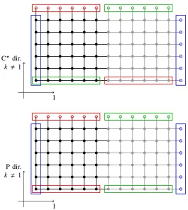
Cboundary conditions in directionsk=2,3 are implemented by modifying the global geometry of the torus. Ifk=2,3 is a Cdirection, then shifted boundary conditions (see fig.1) are imposed
U(x+Lkeˆk, µ)=U(x+L1eˆ1, µ), A(x+Lkˆek, µ)=A(x+L1eˆ1, µ), (11a) ψ(x+Lkˆek)=ψ(x+L1eˆ1), ψ¯(x+Lkˆek)=ψ¯(x+L1eˆ1). (11b)
When combined with the orbifold constraint (4), shifted boundary conditions are equivalent to C boundary conditions in directionk=2,3. For instance for the SU(3) gauge field,
U(x+Lkeˆk, µ)=U(x+L1eˆ1, µ)=U(x, µ)∗. (12)
1 C dir.
k 1
1 P dir.
k 1
Figure 1. Global geometry of extended lattice. Thetop diagramrepresents a section of the extended lattice along a (1,k) plane wherek=2,3 is a Cdirection. All fields are periodic along the extended direction 1. C boundary conditions in the directionk=2,3 are replaced by shifted boundary conditions in the extended lattice. Shifted boundary conditions are imposed by properly defining the nearest neighbours of boundary sites. Empty circles in the red (resp. green, blue) rectangle have to be identified with the corresponding solid circles in the red (resp. green, blue) rectangle. Thebottom diagramrepresents a section of the extended lattice along a (1,k) plane wherek=2,3 is a periodic direction. Inboth diagrams, the black circles represent the sites of the physical
lattice, and the grey circles represent the sites of the mirror lattice.
2.2 Gauge actions
For simplicity, periodic boundary conditions in the time direction will be assumed. The SU(3) and compact U(1) gauge actions are respectively:
Sg,SU(3)=ωC
g20 1
k=0
cSU(3)k
C∈Sk
tr [1−U(C)], (13)
Sg,U(1)= ωC 2q2
ele20 1
k=0
cU(1)k
C∈Sk
[1−z(C)], (14)
Given a pathCon the lattice,U(C) andz(C) denote the SU(3) and U(1) parallel transports along C.S0andS1are the sets of all oriented plaquettes and all oriented 1×2 planar loops respectively.
plaquette loops in the extended lattice instead of the physical lattice. The coefficientsc0,1satisfy the
relationc0+8c1 =1. The Wilson action is obtained by choosingc0 =1, the Lüscher–Weisz action
is obtained by choosingc0 = 53, and the Iwasaki action is obtained by choosingc0 = 3.648. The parameterg0is the bare SU(3) gauge coupling, ande0is the bare U(1) gauge coupling in terms of
which the bare fine–structure constant is given by
α0= e
2 0
4π. (15)
In the compact formulation of QED, all electric charges must be integer multiples of some elementary chargeqelwhich is defined in units of the charge of the positron. As discussed in ref. [1],qelappears
as an overall factor in the gauge action and essentially sets the normalization of the U(1) gauge field in the continuum limit. Even though in infinite volumeqel=1/3 would be an appropriate choice in order to simulate quarks, in finite volume with Cboundary conditions one needs to chooseq
el=1/6
in order to construct gauge–invariant interpolating operators for charged hadrons.
2.3 Dirac operator
The Dirac operator can be written as
D=m0+Dw+δDsw+δDb. (16)
whereDw is the (unimproved) Wilson–Dirac operator, δDsw is the Sheikholeslami–Wohlert (SW)
term, andδDbis the time boundaryO(a)-improvement term. For simplicity, periodic boundary
con-ditions in the time direction will be assumed, which meansδDb=0
In presence of electromagnetism, the Dirac operator depends on the electric charge of the quark field. Letqbe the physical electric charge in units ofe(i.e.q=2/3 for the up quark, andq=−1/3 for the down quark). In the compact formulation of QED, all electric charges must be integer multiples of an elementary chargeqel, which appears as a parameter in the U(1) gauge action (14). It is useful
to introduce the integer parameter
ˆ q= q
qel ∈Z. (17)
The Wilson–Dirac operator can be written as
Dw= 3
µ=0
1 2
γµ(∇µ+∇∗µ)− ∇∗µ∇µ
, (18)
where the covariant derivatives are defined as
∇µψ(x)=U(x, µ)z(x, µ)qˆψ(x+µˆ)−ψ(x), (19) ∇∗µψ(x)=ψ(x)−U(x−µ, µˆ )†z(x−µ, µˆ )−ˆqψ(x−µˆ). (20) Notice that the integer parameter ˆq appears in the hopping term of the Wilson–Dirac operator. The SW term is given by
δDsw=cSU(3)sw 3
µ,ν=0
i
4σµνFµν +q cU(1)sw
3
µ,ν=0
i
plaquette loops in the extended lattice instead of the physical lattice. The coefficientsc0,1satisfy the
relationc0+8c1 =1. The Wilson action is obtained by choosingc0 =1, the Lüscher–Weisz action
is obtained by choosingc0 = 53, and the Iwasaki action is obtained by choosingc0 = 3.648. The parameterg0 is the bare SU(3) gauge coupling, ande0 is the bare U(1) gauge coupling in terms of
which the bare fine–structure constant is given by
α0= e
2 0
4π. (15)
In the compact formulation of QED, all electric charges must be integer multiples of some elementary chargeqelwhich is defined in units of the charge of the positron. As discussed in ref. [1],qelappears
as an overall factor in the gauge action and essentially sets the normalization of the U(1) gauge field in the continuum limit. Even though in infinite volumeqel=1/3 would be an appropriate choice in order to simulate quarks, in finite volume with Cboundary conditions one needs to chooseq
el=1/6
in order to construct gauge–invariant interpolating operators for charged hadrons.
2.3 Dirac operator
The Dirac operator can be written as
D=m0+Dw+δDsw+δDb. (16)
whereDw is the (unimproved) Wilson–Dirac operator, δDsw is the Sheikholeslami–Wohlert (SW)
term, andδDbis the time boundaryO(a)-improvement term. For simplicity, periodic boundary
con-ditions in the time direction will be assumed, which meansδDb=0
In presence of electromagnetism, the Dirac operator depends on the electric charge of the quark field. Letqbe the physical electric charge in units ofe(i.e.q=2/3 for the up quark, andq=−1/3 for the down quark). In the compact formulation of QED, all electric charges must be integer multiples of an elementary chargeqel, which appears as a parameter in the U(1) gauge action (14). It is useful
to introduce the integer parameter
ˆ q= q
qel ∈Z. (17)
The Wilson–Dirac operator can be written as
Dw= 3
µ=0
1 2
γµ(∇µ+∇∗µ)− ∇∗µ∇µ
, (18)
where the covariant derivatives are defined as
∇µψ(x)=U(x, µ)z(x, µ)qˆψ(x+µˆ)−ψ(x), (19) ∇∗µψ(x)=ψ(x)−U(x−µ, µˆ )†z(x−µ, µˆ )−ˆqψ(x−µˆ). (20) Notice that the integer parameter ˆqappears in the hopping term of the Wilson–Dirac operator. The SW term is given by
δDsw=cSU(3)sw 3
µ,ν=0
i
4σµνFµν +q cU(1)sw
3
µ,ν=0
i
4σµνAµν. (21)
The SU(3) field tensorFµν (x) and the U(1) field tensorAµν (x) are constructed in terms of the clover plaquette. The explicit expression of the SU(3) field tensor used inopenQ*Dcan be found in ref. [18], while the U(1) field tensor is given here,
Aµν(x)= i 4qelIm
zµν(x)+zµν(x−µˆ)+zµν(x−νˆ)+zµν(x−µˆ−νˆ) , (22)
zµν(x)=z(x, µ)z(x+µ, νˆ )z(x+ν, µˆ )†z(x, ν)†. (23)
The normalization is chosen in such a way that−ie0Aµνˆ (x) is the canonically–normalized field tensor
in the naive continuum limit, and the discretized field tensors are defined to be anti–hermitian. In the openQ*Dcode, it is possible to choose the values for all parameters of the Dirac operator indepen-dently for each flavour. In particular notice that, in presence of electromagnetism, the values ofcSU(3)sw
andcU(1)sw must depend on the electric charge in order to obtainO(a) improvement.
2.4 Pseudofermion action
The sum over the extended lattice introduces a double counting which can be corrected with an extra 1/2 factor in the fermion action:
Sf=12
x∈Λext ¯
ψ(x)Dψ(x)=−1 2
x∈Λext
ψ(x)TCTDψ(x)≡ −12ψTCTDψ , (24)
where the orbifold constraint (8) has been used. By using the properties of theC matrix one easily proves that
D[U,z]T =CD[U∗,z∗]C−1. (25)
If the gauge field respects the orbifold constraint, andT is the translation operator defined in (7), one trivially gets
TD[U∗,z∗]T−1=D[U,z]. (26)
By combining the previous two equations, and by using the fact thatCis anti–symmetric whileT is symmetric, one gets that the matrixCTDis anti–symmetric. The integration over the fermion field yields the Pfaffian ofCTDup to an irrelevant overall factor which will be reabsorbed in the definition of the fermionic integration measure,
[dψ]Λexte− Sf =
[dψ]Λexte 1
2ψTCTDψ =Pf (CTD). (27)
In the continuum limit, the Pfaffian ofCTDis positive [1]. However at fixed lattice spacing, the Pfaffian is shown to be real but it can be negative on rough enough gauge configurations. The absolute value of the Pfaffian ofCTDhas a representation in terms of the determinant of a positive operator (notice that detC=detT =1)
|Pf (CTD)|=|Det (CTD)|1/2=Det (D†D)1/4. (28)
TheopenQ*D-0.9a2code uses even–odd preconditioning. After decomposing the lattice in even and odd sites in the standard way, the Dirac is represented in block form as
D=
Dee Deo
Doe Doo
In terms of the even–odd preconditioned Dirac operator
ˆ
D=Dee−DeoD−1ooDoe, (30)
the absolute value of the Pfaffian can be written as
|Pf (CTD)|=|DetD|1/2=DetDooDet ˆD1/2=|DetDoo|1/2 Det ( ˆD†Dˆ)1/4. (31)
In order to stabilize the configuration generation, theopenQ*D-0.9a2code allows to introduce a parameter ˆµ2and to replace
Det ( ˆD†Dˆ)1/4→Det ( ˆD†Dˆ+µˆ2)1/4, (32)
which can be corrected by introducing a properly–defined reweighting factor in the observables (fol-lowing the strategy of ref. [5]). LetRbe a rational approximation of order [N,N] of
R( ˆD†Dˆ+µˆ2)−1/4. (33)
TheopenQ*D-0.9a2inherits fromopenQCD-1.6the frequency splitting for the RHMC [5]. If the rational approximation is written explicitly as
R=A N
j=1
ˆ D†Dˆ +ν2
j ˆ D†Dˆ +µ2
j
, (34)
where the finite sequencesµj andνj are assumed to be monotonically increasing, one can always define a factorization
R=A P1P2· · ·Pn, (35)
where the factorsPkcontain all the zeroes and poles with indices in a given range{Jk,Jk+1, . . . ,Jk+1− 1}, i.e.
Pk= Jk+1−1
j=Jk
ˆ D†Dˆ +ν2
j ˆ D†Dˆ+µ2
j
. (36)
TheopenQ*D-0.9a2code simulates the absolute value of the Pfaffian by means of the pseud-ofermion action given by
|Pf (CT D)| |DetDoo|1/2 DetR−1=
[dφdφ∗]even(Λext)e−Spf, (37)
Spf=−12ln|DetDoo|+
n
k=1
φ†kPkφk. (38)
The pseudofermionφkis a complex field with gauge and spinor indices, which lives on the even sites of the extended lattice. It satisfies periodic boundary conditions in direction 1, and possibly shifted boundary condition in directionsk = 2,3. It is completely unrestricted over the extended lattice.
In terms of the even–odd preconditioned Dirac operator
ˆ
D=Dee−DeoD−1ooDoe, (30)
the absolute value of the Pfaffian can be written as
|Pf (CTD)|=|DetD|1/2 =DetDooDet ˆD1/2 =|DetDoo|1/2 Det ( ˆD†Dˆ)1/4. (31)
In order to stabilize the configuration generation, theopenQ*D-0.9a2code allows to introduce a parameter ˆµ2and to replace
Det ( ˆD†Dˆ)1/4→Det ( ˆD†Dˆ +µˆ2)1/4, (32)
which can be corrected by introducing a properly–defined reweighting factor in the observables (fol-lowing the strategy of ref. [5]). LetRbe a rational approximation of order [N,N] of
R( ˆD†Dˆ +µˆ2)−1/4. (33)
TheopenQ*D-0.9a2inherits fromopenQCD-1.6the frequency splitting for the RHMC [5]. If the rational approximation is written explicitly as
R=A N
j=1
ˆ D†Dˆ +ν2
j ˆ D†Dˆ+µ2
j
, (34)
where the finite sequencesµj andνj are assumed to be monotonically increasing, one can always define a factorization
R=A P1P2· · ·Pn, (35)
where the factorsPkcontain all the zeroes and poles with indices in a given range{Jk,Jk+1, . . . ,Jk+1− 1}, i.e.
Pk= Jk+1−1
j=Jk
ˆ D†Dˆ+ν2
j ˆ D†Dˆ +µ2
j
. (36)
TheopenQ*D-0.9a2code simulates the absolute value of the Pfaffian by means of the pseud-ofermion action given by
|Pf (CT D)| |DetDoo|1/2 DetR−1 =
[dφdφ∗]even(Λext)e−Spf , (37)
Spf=−12ln|DetDoo|+
n
k=1
φ†kPkφk. (38)
The pseudofermionφkis a complex field with gauge and spinor indices, which lives on the even sites of the extended lattice. It satisfies periodic boundary conditions in direction 1, and possibly shifted boundary condition in directionsk = 2,3. It is completely unrestricted over the extended lattice.
Notice that, sinceDoois diagonal in the lattice index, its determinant can be calculated exactly.
2.5 Molecular dynamics
The momentum fields associated to the SU(3) and U(1) gauge field are denoted byΠ(x, µ) andπ(x, µ) respectively. The momentumΠ(x, µ) lives in the Lie algebra of SU(3),
Π(x, µ)= Πa(x, µ)Ta, (39)
whereΠa(x, µ) are taken to be real. The momentum fieldπ(x, µ) is taken to be real, like the gauge
fieldA(x, µ). With Cboundary conditions, the momentum fields must satisfy the orbifold constraint
Π(x+L1eˆ1, µ)= Π(x, µ)∗, π(x+L1eˆ1, µ)=−π(x, µ). (40)
Summing over all momenta in the extended lattice instead of the physical lattice introduces a double counting which can be corrected with an extra 1/2 factor in the MD Hamiltonian:
H=1 4
x,µ
[π(x, µ)]2+ a
[Πa(x, µ)]2+S(U,A). (41)
In deriving the MD equations, one needs to take into account the orbifold constraint. It is conve-nient to define the forces as the derivative of the actionS(U,A) thought as a function of the uncon-strained fields on the extended lattice
F(x, µ)=−∂U(x,µ)S(U,A)
unconstrained , f(x, µ)=−
∂A(x,µ)S(U,A)
unconstrained . (42)
By using the orbifold constraint and the chain rule, the MD equations are found to be
∂tU(x, µ)= Π(x, µ)U(x, µ), ∂tΠ(x, µ)=F(x, µ)+F(x+L1eˆ1, µ)∗, (43a) ∂tA(x, µ)=π(x, µ), ∂tπ(x, µ)= f(x, µ)−f(x+L1eˆ1, µ). (43b)
Since the Hamiltonian is invariant under translations and charge–conjugation, the orbifold constraint is preserved by the MD. In fact the orbifold constraint is also preserved by the discrete integrators used by theopenQ*Dcode.
3 QCD: some tests
We have performed some test runs in order to assess two issues: • the overhead due to the orbifold construction;
• the effectiveness of deflation with Cboundary conditions.
The results presented here allow only to scratch the surface of these issues. The drawn conclusion are far from definitive and should be taken with a grain of salt.
All runs presented in this section share the following parameters: • QCD withNf =2 degenerate flavours;
• Physical lattice 64×323with periodic boundary conditions in time;
• Wilson action withβ=5.2;
• Non–perturbativelyO(a) improved Wilson fermions withκ=0.1359 andcsw=2.017147;
• MD trajectory lenghtτ=2;
• a0.08 fm,mπ380 MeV,mπL4.7.
3.1 Overhead due to the orbifold construction
A possible and direct way to implement C boundary conditions is to pack the quark and antiquark into a doublet
Ψ =
ψ
C−1ψ¯T
, (44)
which transform under theׯ representation of the gauge group. The boundary conditions swap the two components ofΨ. When the pseudofermion action is derived, pseudofermions will have two components as well. Let us denote byDC,2cthe Dirac operator with Cboundary conditions in the
2-component formulation. The Dirac operator acts independently on the two components in the bulk and mixes the two components at the boundary.
InopenQ*D-0.9a2, Cboundary conditions are implemented through an orbifold construction. The Dirac operatorDC,orbiacts on single–component pseudofermions which are defined on a lattice
that is twice as large as the physical lattice.
The orbifold construction was preferred to the two–component formulation for the openQ*D-0.9a2code, since it required no modification of the Dirac operator and solvers of the originalopenQCD-1.6code. The implementation of C boundary conditions via the orbifold con-struction is almost trivial. However, one may think that simulations with the orbifold concon-struction are much more expensive. The question we want to address is:how more expensive is the orbifold construction with respect to the two–component construction?
If the physical volumeV =T L3is kept constant it is obvious that
cost[DC,2cΦ2c,V]=cost[DC,orbiφ2c,2V]=2 cost[DPφ1c,V]{1+O(L−1)}, (45)
whereDPis the standard operator with periodic boundary conditions, which acts on single–component
pseudofermions. Therefore, the application of the Dirac operator and the solution of the Dirac equa-tion has exactly the same cost in the two possible implementaequa-tions of Cboundary conditions.
The orbifold construction loses for two reasons:
• The gauge fields are evolved twice, in the physical and mirror lattice, see fig.1. This operation is relatively cheap, but it is done many times (at the innermost level of the integrator).
• The forces in the physical and mirror lattices need to be summed in the evolution equations for the momenta, see eqs. (43), and this requires MPI communications. TheopenQ*D-0.9a2code implements two solutions to mitigate this issue. First we notice that the gauge force (which is integrated more often) satisfies automatically the orbifold constraint. The sum of forces in eqs. (43) gives a trivial factor of two for the gauge force. As a second measure, the MPI ranks are organized in such a way that a pointxand its mirror pointx+L1eˆ1 belong to different MPI processes, but end up on the same multi–core node (assuming an MPI implementation for which MPI processes residing on a node are numbered consecutively). In this case the MPI communications needed for eqs. (43) should not go through the network.
The cost for the gauge field and momenta evolution is identical in the 2-component implementation of the Cboundary conditions and in the periodic case. Assuming that the volume is large enough, the cost of the simulation of the theory with periodic boundary conditions is going to be equal to the cost of the simulation of the theory with Cboundary conditions implemented with the 2-component for-malism, provided that all parameters of the algorithm are identical (in particular the RHMC algorithm is used in both cases, and the rational approximation is the same).
3.1 Overhead due to the orbifold construction
A possible and direct way to implement Cboundary conditions is to pack the quark and antiquark into a doublet
Ψ =
ψ
C−1ψ¯T
, (44)
which transform under theׯ representation of the gauge group. The boundary conditions swap the two components ofΨ. When the pseudofermion action is derived, pseudofermions will have two components as well. Let us denote byDC,2c the Dirac operator with Cboundary conditions in the
2-component formulation. The Dirac operator acts independently on the two components in the bulk and mixes the two components at the boundary.
InopenQ*D-0.9a2, Cboundary conditions are implemented through an orbifold construction. The Dirac operatorDC,orbiacts on single–component pseudofermions which are defined on a lattice
that is twice as large as the physical lattice.
The orbifold construction was preferred to the two–component formulation for the openQ*D-0.9a2 code, since it required no modification of the Dirac operator and solvers of the originalopenQCD-1.6code. The implementation of C boundary conditions via the orbifold con-struction is almost trivial. However, one may think that simulations with the orbifold concon-struction are much more expensive. The question we want to address is:how more expensive is the orbifold construction with respect to the two–component construction?
If the physical volumeV=T L3is kept constant it is obvious that
cost[DC,2cΦ2c,V]=cost[DC,orbiφ2c,2V]=2 cost[DPφ1c,V]{1+O(L−1)}, (45)
whereDPis the standard operator with periodic boundary conditions, which acts on single–component
pseudofermions. Therefore, the application of the Dirac operator and the solution of the Dirac equa-tion has exactly the same cost in the two possible implementaequa-tions of Cboundary conditions.
The orbifold construction loses for two reasons:
• The gauge fields are evolved twice, in the physical and mirror lattice, see fig.1. This operation is relatively cheap, but it is done many times (at the innermost level of the integrator).
• The forces in the physical and mirror lattices need to be summed in the evolution equations for the momenta, see eqs. (43), and this requires MPI communications. TheopenQ*D-0.9a2code implements two solutions to mitigate this issue. First we notice that the gauge force (which is integrated more often) satisfies automatically the orbifold constraint. The sum of forces in eqs. (43) gives a trivial factor of two for the gauge force. As a second measure, the MPI ranks are organized in such a way that a point xand its mirror point x+L1eˆ1 belong to different MPI processes, but end up on the same multi–core node (assuming an MPI implementation for which MPI processes residing on a node are numbered consecutively). In this case the MPI communications needed for eqs. (43) should not go through the network.
The cost for the gauge field and momenta evolution is identical in the 2-component implementation of the Cboundary conditions and in the periodic case. Assuming that the volume is large enough, the cost of the simulation of the theory with periodic boundary conditions is going to be equal to the cost of the simulation of the theory with Cboundary conditions implemented with the 2-component for-malism, provided that all parameters of the algorithm are identical (in particular the RHMC algorithm is used in both cases, and the rational approximation is the same).
Then the overhead due to the orbifold construction is obtained by comparing the run with periodic boundary conditions (QCD2) with the run with Cboundary conditions implemented with the orbifold
construction (QCD3). For details about these runs, refer to app.A. By comparing the simulation times listed in table1, we conclude that the orbifold construction produces a relative overhead in cost of about 1%. The relative overhead is expected to decrease at smaller quark masses (since the solution of the Dirac equation becomes more expensive relatively to the gauge field and momenta evolution).
3.2 RHMC vs. HMC
In the case ofNf =2 degenerate flavours and periodic boundary conditions in space, one can use the HMC algorithm. We have generated the QCD1 ensemble with the HMC and twisted–mass Hasen-busch preconditioning, with splitting of the various terms in different integration levels.
In case of Cboundary conditions one is forced to use the RHMC since the Pfaffian needs to be simulated. We use a representation of the Pfaffian of the type
|Pf (CTD)|2 = 1
Det (D†D)−1/4
1
Det (D†D)−1/4 , (46)
with a rational approximation for (D†D)−1/4, as this is more similar to the setup needed for the
in-clusion of isospin–breaking corrections. We have generated the QCD3 ensemble with Cboundary conditions, the RHMC with a rational approximation for (D†D)−1/4and frequency splitting in different
integration levels.
For details about the QCD1 and QCD3 runs, refer to app.A. By comparing the simulation times listed in table1, we see that the QCD3 run is about 5.5 times slower than the QCD1 run. This big factor is most likely an indication of the fact that the QCD3 run has not been optimized as well as the QCD1 run. We plan to invest more time into the optimization of the RHMC runs, and in particular we thank Kate Clark for providing useful suggestions during the conference.
4 QCD+QED: some tests
We have also usedopenQ*D-0.9a2code to perform test runs that include the dynamical degrees of freedom of the U(1) gauge field. The aim of these runs was twofold:
• to examine whether any unexpected features appear if compact QCD+QED simulations are per-formed with Wilson fermions and Cboundary conditions;
• to get a first insight into autocorrelations of SU(3) and U(1) gauge observables.
TheopenQ*D-0.9a2code currently implements only the compact formulation of QED; hence, we perform the initial tests with the compact QED action. The test runs presented in this section share the following parameters:
• QCD+QED withNf =2+1 fermion flavours; • Cbc’s in all space directions;
• αem=0.05≈7αphysem ;
• Lüscher–Weisz SU(3) gauge action and Wilson U(1) gauge action;
• Wilson fermion action with SU(3) SW–term coefficients determined atαem=0;
• Tree–level coefficients for the U(1) SW–term;
6.00 6.20 6.40 6.60 6.80 7.00
0 500 1000 1500 2000 2500 3000
λmax
Ncnfg
q=-1/3 q=2/3 QCD+QED1
5.60 5.80 6.00 6.20 6.40 6.60 6.80 7.00
0 5000 10000
λmax
Ncnfg
q=-1/3 q=2/3 QCD+QED2
0.02 0.04 0.06 0.08 0.10
0 1000 2000 3000
λmin
Ncnfg
q=-1/3 q=2/3 QCD+QED1
0.05 0.10 0.15 0.20 0.25 0.30
0 5000 10000
λmin
Ncnfg
q=-1/3 q=2/3 QCD+QED2
Figure 2. Spectral ranges of|γ5D|in the performed QCD+QED simulations.Theupper panelsrepresent the
estimate of the highest eigenvalue of|γ5D|corresponding to thed/squarks (red) anduquark (blue). Similarly,
thelower panelsrepresent the evolution of the estimated smallest eigenvalues.
The first run (QCD+QED1) takes over the parameters from the H200 ensemble of theNf =2+1 CLS [21], except that the lattice extent is halved in each of the space–time directions. The dynamical U(1) degrees of freedom contribute to the renormalization of the bare parameters, hence the estimate for the lattice spacing and pion mass cannot be taken from the CLS ensembles1, but rather need to be estimated independently.
The parameters characteristic for each of the performed QCD+QED runs are the following: • QCD+QED1: Physical lattice 32×163with periodic bc’s in time,β=3.55,cSU(3)
sw,u =cSU(3)sw,d =cSU(3)sw,s =
1.824865,κu=κd=κs=0.137;
• QCD+QED2: Physical lattice 16×83with open–SF bc’s in time;β=4.0,cSU(3)
sw,u =cSU(3)sw,d =cSU(3)sw,s =
1.540714371185832,κu=κd =κs=0.136646552997824;.
AlthoughopenQ*D-0.9a2code allows for twisted–mass reweighting, the runs described in this sec-tion do not use that opsec-tion (ˆµ=0.0). In both runs all three bare sea quark masses are taken to be the same. However, due to the differences in quark charges we end up with a degenerate pair of quarks (down and strange) withq =−1/3, and a single quark (up) withq =2/3 in our simulations; hence, we are essentially simulatingNf =2+1 theory.
4.1 Spectral ranges of the Dirac operators
We monitored the smallest and the largest eigenvalue of|γ5Du|and|γ5Dd/s|throughout the performed QCD+QED runs, in order to confirm that the spectral ranges of the rational approximations have been
1Had the U(1) d.o.f. been switched off(αem=0), the chosen parameter set would correspond tom
6.00 6.20 6.40 6.60 6.80 7.00
0 500 1000 1500 2000 2500 3000
λmax Ncnfg q=-1/3 q=2/3 QCD+QED1 5.60 5.80 6.00 6.20 6.40 6.60 6.80 7.00
0 5000 10000
λmax Ncnfg q=-1/3 q=2/3 QCD+QED2 0.02 0.04 0.06 0.08 0.10
0 1000 2000 3000
λmin Ncnfg q=-1/3 q=2/3 QCD+QED1 0.05 0.10 0.15 0.20 0.25 0.30
0 5000 10000
λmin
Ncnfg
q=-1/3 q=2/3 QCD+QED2
Figure 2. Spectral ranges of|γ5D|in the performed QCD+QED simulations.Theupper panelsrepresent the
estimate of the highest eigenvalue of|γ5D|corresponding to thed/squarks (red) anduquark (blue). Similarly,
thelower panelsrepresent the evolution of the estimated smallest eigenvalues.
The first run (QCD+QED1) takes over the parameters from the H200 ensemble of theNf =2+1 CLS [21], except that the lattice extent is halved in each of the space–time directions. The dynamical U(1) degrees of freedom contribute to the renormalization of the bare parameters, hence the estimate for the lattice spacing and pion mass cannot be taken from the CLS ensembles1, but rather need to be estimated independently.
The parameters characteristic for each of the performed QCD+QED runs are the following: • QCD+QED1: Physical lattice 32×163with periodic bc’s in time,β=3.55,cSU(3)
sw,u =cSU(3)sw,d =cSU(3)sw,s =
1.824865,κu=κd =κs=0.137;
• QCD+QED2: Physical lattice 16×83with open–SF bc’s in time;β=4.0,cSU(3)
sw,u =cSU(3)sw,d =cSU(3)sw,s =
1.540714371185832,κu =κd=κs=0.136646552997824;.
AlthoughopenQ*D-0.9a2code allows for twisted–mass reweighting, the runs described in this sec-tion do not use that opsec-tion (ˆµ=0.0). In both runs all three bare sea quark masses are taken to be the same. However, due to the differences in quark charges we end up with a degenerate pair of quarks (down and strange) withq =−1/3, and a single quark (up) withq =2/3 in our simulations; hence, we are essentially simulatingNf =2+1 theory.
4.1 Spectral ranges of the Dirac operators
We monitored the smallest and the largest eigenvalue of|γ5Du|and|γ5Dd/s|throughout the performed QCD+QED runs, in order to confirm that the spectral ranges of the rational approximations have been
1Had the U(1) d.o.f. been switched off(αem=0), the chosen parameter set would correspond tom
π≈420 MeV.
-8 -6 -4 -2 0 2 4 6 8
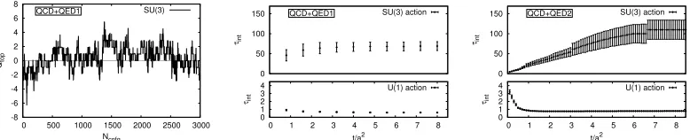
0 500 1000 1500 2000 2500 3000 Qtop Ncnfg SU(3) QCD+QED1 0 50 100 150 τint SU(3) action QCD+QED1 0 1 2 3 4
0 1 2 3 4 5 6 7 8 τint t/a2 U(1) action 0 50 100 150 τint SU(3) action QCD+QED2 0 1 2 3 4
0 1 2 3 4 5 6 7 8 τint
t/a2
U(1) action
Figure 3. Autocorrelations in the performed QCD+QED simulations.Theleft panelshows the history of the SU(3) topological charge defined in eq. (54), measured on thermalized configurations in theQCD+QED1ensemble at the flow timetdefined by √8t=0.3×L, and corresponding tot/a2=0.36. The remaining plots compare the
autocorrelations of the SU(3) and U(1) observables in theQCD+QED1run with periodic bc’s in time (middle panel) and in the small volumeQCD+QED2run with open–SF bc’s in time (right panel). All runs feature Cspatial bc’s.
chosen correctly. It turns out that, subsequent to the thermalization phase, the inclusion of electro-magnetic effects does not lead to large fluctuations of the spectral range. The results of the estimated spectral ranges in runsQCD+QED1 (left panels) andQCD+QED2(right panels) are shown in fig.2. See app.Bfor details on the chosen spectral ranges in the corresponding rational approximations.
4.2 Autocorrelations of SU(3) and U(1) gauge observables
We use Wilson flow to define the global topological charge and the action density for SU(3) and U(1) gauge fields (see app.Band ref. [22]). In the left panel of fig.3we show the history ofQtop(t) in the
ensembleQCD+QED1, while the flow time dependence of autocorrelation times of the U(1) and SU(3) action in the same run are shown in the middle panel of fig.3. The flow timetin the plottedQtop(t)
is chosen such that√8t=0.3×L. TheQCD+QED1 run features periodic boundary conditions in time and the length of the run seems not to be sufficient to give a reliable estimate of the autocorrelations of the global topological charge. This motivated the choice of input parameters for our second ensemble: open–SF bc’s in time, and much smaller volume in physical units (smaller lattice 83×16 and larger
value ofβ). The statistics gathered in theQCD+QED2 run O(10000) allows for a good estimate of how fast the Wilson flow quantities decorrelate in the QCD+QED simulations with Cspace bc’s. The autocorrelations of the U(1) and SU(3) action, see eqs. (52) and (53), for the runQCD+QED2 are shown in the right panel of fig.3. Notice that for both choices of bc’s in time, the autocorrelations of U(1) observables are ofO(1) even though we are not using any technique to decrease the U(1) field autocorrelations, such as Fourier acceleration.
Acknowledgements.Most simulations reported in this paper were performed on a dedicated PC
A Some details on the QCD test runs
We have produced three ensembles which differ by the space boundary conditions (and consequently by the simulated lattice) and by the algorithm used, as summarized in table1. In all cases, a 3–level integrator has been used, following the strategy used in ref. [21]:
• 1 steps of 4th order OMF integrator in the innermost level (level 0); • 1 step of 4th order OMF integrator in the intermediate level (level 1);
• 12 step of 2nd order OMF integrator withλ=1/6 in the outermost level (level 2).
Only the gauge force is integrated in level 0, while the fermionic forces are distributed in levels 1 and 2, in different ways depending on the particular algorithm used. In all cases the acceptance rate is found to be between 90% and 95%. Let us look now in detail at the algorithms used for each run listed in table1.
Table 1.Nf =2 QCD test runs (a0.08 fm,mπ380 MeV,mπL4.7). Notice that, in case of Cboundary conditions, the global lattice is larger than physical lattice because of the orbifold contruction.
Run name Space bc’s Global lattice Local lattice Algorithm Time/trajs
QCD1 periodic 64×323 8×83 HMC+TM 600s
QCD2 periodic 64×323 8×83 RHMC–4×1/4 3890s
QCD3 Cin 3 dirs 64×64×322 8×16×82 RHMC–2×1/4 3920s
QCD1. In case of periodic boundary conditions, one can use the HMC algorithm with even–odd and Hasenbusch twisted–mass preconditioning. We use a pseudofermion action of the form
Spf=Spf,1+Spf,2, (47)
Spf,1=−2 ln|detDoo|+φ†3 1
ˆ
D†Dˆ +µ3φ3+φ † 2
ˆ D†Dˆ+µ3
ˆ
D†Dˆ+µ2φ2+φ † 1
ˆ D†Dˆ +µ2
ˆ
D†Dˆ +µ1φ1, (48)
Spf,2=φ†0
ˆ D†Dˆ+µ1
ˆ
D†Dˆ+µˆ φ0. (49)
We choose (µ1, µ2, µ3)=(0.005,0.05,0.5). The force associated toSpf,1is integrated in level 1, while
the force associated toSpf,2is integrated in level 2. The Dirac equation is solved by means of a
conjugate gradient for twisted massµ=0.5 and by means of the deflation–accelerated solver in all other cases.
QCD2. In case of periodic boundary conditions, one can use the RHMC algorithm with multiple copies of pseudofermion fields. In particular, we construct the optimal rational approximation with relative precision of 10−6for
( ˆD†Dˆ+µˆ2)−1/4, (50)
assuming that the spectrum of|γ5Dˆ|is included in the range [1.98×10−3,7.62]. We split the rational
approximation in 8 factors, as explained in subsection2.4. The forces associated to different factors are integrated in different levels. Also different solvers are used to solve the Dirac equations associated to the different factors. These details are summarized in table2. The pseudofermion action reads
Spf=−N2pfln|DetDoo|+
Npf
α=1 8
k=1
A Some details on the QCD test runs
We have produced three ensembles which differ by the space boundary conditions (and consequently by the simulated lattice) and by the algorithm used, as summarized in table1. In all cases, a 3–level integrator has been used, following the strategy used in ref. [21]:
• 1 steps of 4th order OMF integrator in the innermost level (level 0); • 1 step of 4th order OMF integrator in the intermediate level (level 1);
• 12 step of 2nd order OMF integrator withλ=1/6 in the outermost level (level 2).
Only the gauge force is integrated in level 0, while the fermionic forces are distributed in levels 1 and 2, in different ways depending on the particular algorithm used. In all cases the acceptance rate is found to be between 90% and 95%. Let us look now in detail at the algorithms used for each run listed in table1.
Table 1.Nf =2 QCD test runs (a0.08 fm,mπ380 MeV,mπL4.7). Notice that, in case of Cboundary conditions, the global lattice is larger than physical lattice because of the orbifold contruction.
Run name Space bc’s Global lattice Local lattice Algorithm Time/trajs
QCD1 periodic 64×323 8×83 HMC+TM 600s
QCD2 periodic 64×323 8×83 RHMC–4×1/4 3890s
QCD3 Cin 3 dirs 64×64×322 8×16×82 RHMC–2×1/4 3920s
QCD1. In case of periodic boundary conditions, one can use the HMC algorithm with even–odd and Hasenbusch twisted–mass preconditioning. We use a pseudofermion action of the form
Spf=Spf,1+Spf,2, (47)
Spf,1=−2 ln|detDoo|+φ†3 1
ˆ
D†Dˆ +µ3φ3+φ † 2
ˆ D†Dˆ+µ3
ˆ
D†Dˆ+µ2φ2+φ † 1
ˆ D†Dˆ +µ2
ˆ
D†Dˆ +µ1φ1, (48)
Spf,2=φ†0
ˆ D†Dˆ+µ1
ˆ
D†Dˆ+µˆ φ0. (49)
We choose (µ1, µ2, µ3)=(0.005,0.05,0.5). The force associated toSpf,1is integrated in level 1, while
the force associated toSpf,2 is integrated in level 2. The Dirac equation is solved by means of a
conjugate gradient for twisted massµ =0.5 and by means of the deflation–accelerated solver in all other cases.
QCD2. In case of periodic boundary conditions, one can use the RHMC algorithm with multiple copies of pseudofermion fields. In particular, we construct the optimal rational approximation with relative precision of 10−6for
( ˆD†Dˆ +µˆ2)−1/4, (50)
assuming that the spectrum of|γ5Dˆ|is included in the range [1.98×10−3,7.62]. We split the rational
approximation in 8 factors, as explained in subsection2.4. The forces associated to different factors are integrated in different levels. Also different solvers are used to solve the Dirac equations associated to the different factors. These details are summarized in table2. The pseudofermion action reads
Spf=−N2pfln|DetDoo|+
Npf
α=1 8
k=1
φ†α,kPkφα,k, (51)
Table 2.Rational approximation used for the QCD2 and QCD3 runs. Each zero/pole pair is included in a
frequency–splitting (FS) factorPk, the corresponding pseudofermion force is integrated in either level 1 or level
2, and different solvers are used to solve the associated Dirac equations.
j νj µj FS factor Integration level Solver
1 1.7626×10+01 1.2383×10+01 P
1 level 1
Multi–shift CG 2 5.9094×10+00 4.8370×10+00 P1 level 1
3 2.7961×10+00 2.3515×10+00 P
1 level 1
4 1.4167×10+00 1.1994×10+00 P
1 level 1
5 7.3020×10−01 6.1927×10−01 P
1 level 1
6 3.7808×10−01 3.2079×10−01 P
1 level 1
7 1.9600×10−01 1.6632×10−01 P
1 level 1
8 1.0163×10−01 8.6246×10−02 P
2 level 1 Deflation–accelerated
9 5.2700×10−02 4.4718×10−02 P
3 level 2 Deflation–accelerated
10 2.7313×10−02 2.3170×10−02 P
4 level 2 Deflation–accelerated
11 1.4128×10−02 1.1973×10−02 P
5 level 2 Deflation–accelerated
12 7.2571×10−03 6.1273×10−03 P
6 level 2 Deflation–accelerated
13 3.6347×10−03 3.0301×10−03 P
7 level 2 Deflation–accelerated
14 1.6921×10−03 1.3855×10−03 P
8 level 2 Deflation–accelerated
whereNpf=4 copies of pseudofermion fields have been used in order to reproduce the correct number of flavours.
QCD3. In case of C boundary conditions, one must use the RHMC algorithm with multiple copies of pseudofermion fields. We use the same setup as for the QCD2 run (see table2) with the only difference that in this case the correct number of flavours is obtained by usingNpf=2 copies of pseudofermion fields.
B Some details on the QCD+QED test runs
We have produced two ensembles which differ by the time boundary conditions and by the lattice size. The algorithm used in all cases is the same (RHMC) and involves a 3–level integrator:
• 1 step of 4th order OMF integrator in the innermost level (level 0); • 3 steps of 4th order OMF integrator in the intermediate level (level 1); • 10 steps of 4th order OMF integrator in the outermost level (level 2).
The U(1) force is integrated in level 0, the SU(3) force in level 1, and all the fermionic forces are integrated in the outermost level (level 2). The two runs are simulating C bc’s in space and the Dirac equation is solved by means of CG in all cases (multi–shift CG is used for all the factors in
Table 3.Nf =2+1 QCD+QED test runs. N represents the order of the corresponding rational approximation,
and [λmin, λmax] is the range that is assumed to include the spectrum of|γ5Dˆ|in both cases.
Run name Time bc’s Lattice (D†D)−1/2 (D†D)−1/4 N
cnfg
N [λmin, λmax] N [λmin, λmax]
QCD+QED1 periodic 32×163 20 [9.17×10−3,6.94] 16 [3.65×10−2,6.94] 3000
the rational approximation). See table3for details on the degrees and spectral ranges of the rational approximation used for the (D†D)−1/4(up quark) and (D†D)−1/2(down and strange quarks).
The SU(3) and U(1) action densities are defined as:
ESU(3)(t) = 2L13T
x
µν
tr{Fµν (x,t)Fµν (x,t)}, (52)
EU(1)(t) = 2L13T
x
µν
tr{Aµν(x,t)Aµν (x,t)}, (53)
whereFµν (x,t) andAµν (x,t) are the clover–type discretization of the SU(3) and U(1) field strength tensors respectively, at positive flow time. The global topological charge for SU(3) gauge fields is given by:
Qtop(t) = 321π2
x
µνρσ
µνρσtr{Fµν (x,t)Fρσ (x,t)}. (54)
References
[1] B. Lucini, A. Patella, A. Ramos, N. Tantalo, JHEP02, 076 (2016),1509.01636
[2] G.M. de Divitiis, R. Frezzotti, V. Lubicz, G. Martinelli, R. Petronzio, G.C. Rossi, F. Sanfilippo, S. Simula, N. Tantalo (RM123), Phys. Rev.D87, 114505 (2013),1303.4896
[3] M. Hansen, B. Lucini, A. Patella, N. Tantalo,Simulations of QCD and QED with C bound-ary conditions, in Proceedings, 35th International Symposium on Lattice Field Theory (Lat-tice2017): Granada, Spain(2018), Vol. unknown
[4] http://cern.ch/luscher/openQCD
[5] M. Lüscher, S. Schaefer, Comput. Phys. Commun.184, 519 (2013),1206.2809
[6] M. Lüscher, P. Weisz, Commun. Math. Phys. 97, 59 (1985), [Erratum: Commun. Math. Phys.98,433(1985)]
[7] Y. Iwasaki (1983),1111.7054
[8] B. Sheikholeslami, R. Wohlert, Nucl. Phys.B259, 572 (1985) [9] U.J. Wiese, Nucl. Phys.B375, 45 (1992)
[10] J.C. Sexton, D.H. Weingarten, Nucl. Phys.B380, 665 (1992)
[11] I. Omelyan, I. Mryglod, R. Folk, Computer Physics Communications151, 272 (2003) [12] M. Hasenbusch, Phys. Lett.B519, 177 (2001),hep-lat/0107019
[13] M. Hasenbusch, K. Jansen, Nucl. Phys.B659, 299 (2003),hep-lat/0211042 [14] T.A. DeGrand, Comput. Phys. Commun.52, 161 (1988)
[15] A.D. Kennedy, I. Horvath, S. Sint, Nucl. Phys. Proc. Suppl.73, 834 (1999),hep-lat/9809092 [16] M. Lüscher, JHEP07, 081 (2007),0706.2298
[17] M. Lüscher, JHEP12, 011 (2007),0710.5417
[18] M. Lüscher, S. Sint, R. Sommer, P. Weisz, Nucl. Phys.B478, 365 (1996),hep-lat/9605038 [19] P. Fritzsch, F. Knechtli, B. Leder, M. Marinkovic, S. Schaefer, R. Sommer, F. Virotta, Nucl.
Phys.B865, 397 (2012),1205.5380
[20] K. Jansen, R. Sommer (ALPHA), Nucl. Phys. B530, 185 (1998), [Erratum: Nucl. Phys.B643,517(2002)],hep-lat/9803017
[21] M. Bruno et al., JHEP02, 043 (2015),1411.3982


![Table 3. Nf = 2 + 1 QCD+QED test runs. N represents the order of the corresponding rational approximation,and [λmin, λmax] is the range that is assumed to include the spectrum of |γ5 Dˆ| in both cases.](https://thumb-us.123doks.com/thumbv2/123dok_us/8056182.1342531/15.482.46.433.592.651/table-represents-corresponding-rational-approximation-assumed-include-spectrum.webp)
