Article
1
Revisiting the relationship between financial wealth,
2
housing wealth and consumption: a panel analysis for
3
the US
4
Dimitra Kontana * and Fotios Siokis
5
University of Macedonia, Egnatia 156, Thessaloniki, Greece
6
* Correspondence: d.kontana@uom.edu.gr; Tel.: +xx-xxx-xxx-xxxx
7
8
Abstract: Based on the seminal paper of Case, Quigley and Shiller (2013), we investigate the
9
effects of financial and housing wealth on consumption. Using quarterly data from 1975 to 2016,
10
for all States of U.S. economy, and a different methodology in measuring wealth, we report
11
relatively greater financial effects than housing effects on consumption. Specifically, in our basic
12
utilized model, the calculated elasticity for financial wealth is 0.060, while for housing is 0.045. The
13
results are not in agreement with the ones obtained by Case, Quigley and Shiller. In an attempt to
14
investigate the disparity we proceed by incorporating the introduction of the Tax Reform Act in
15
1986, which increased incentives for owner-occupied housing investments. Finally, due to
16
distributional factors at work, and taking into account the pronounced uneven distribution of wealth
17
we investigate the effects of wealth for 8 states that include the Metropolitan areas comprising of the
18
well known Case-Shiller 10-City Composite Index. Now the housing effect on consumption is
19
much stronger and larger than the financial effect. Additionally, we forecast the consumption
20
changes at the time of the high rise and large drops in house prices for these states. Forecasts
21
showed a recession from the fall of Lehman Brothers until the fourth quarter of 2011. These
22
forecasts were not verified. Probably, the new techniques used by politics played an important
23
role. We also find that extreme behaviors cannot be predicted.
24
JEL codes. E21; E44; R31.
25
Keywords. Consumption; Financial Wealth; Housing Wealth; Wealth effects.
26
1. Introduction
27
The pronounced volatility in the prices of financial assets, and in the housing prices, during the
28
period from 2002 to 2009 and, consequently the effects of the Great Recession in the economy, has
29
led to renewed political and scientific interest in the effect of wealth on aggregate consumption.
30
The enormous swings in wealth, either from financial wealth or property wealth have grown in
31
importance and raised a number of questions about the macroeconomic implications on consumer
32
spending, aggregate demand and consequently on economic activity. Declines in stock prices
33
accelerate the slowdown of households consumption and thus of the economic activity, a process
34
which, eventually could lead to a recession. The same importance yields the changes in housing
35
wealth upon household behavior, since recent developments in the housing markets give the
36
opportunity to the homeowner to extract cash from housing and use it for consumption.
37
Against this backdrop, it is not surprisingly that some researchers state that housing equity is
38
essentially similar to the act of selling shares. But in contrast to that, other researchers point out
39
that the impact of stock market wealth accumulation may be quite different from that of real estate,
40
because people may be less aware of the short - term changes in real estate market, since they do not
41
receive relevant updates on its value. As for the financial wealth, people have immediate
42
information on changes in the stock market through the news, online, or from newspapers.
43
While in the last couple of decades the impact of wealth on consumption has been studied
44
extensively, still, there is no clear consensus of whether housing wealth effects are greater than
45
financial wealth effects. Equally, the theoretical underpinnings of the housing wealth effect remain
46
controversial. Buiter (2010) suggests that housing wealth is not really wealth, and even if it is the
47
effects are not of primary importance. Under a standard life-cycle permanent income consumption
48
model, he argues that housing wealth is considered at the same time an asset and consumption
49
good, and housing consumption costs offset any housing wealth effect on consumption, leaving thus
50
overall consumption unchanged. Most efforts support the notion that housing wealth is a reliable
51
indicator of business cycle and therefore an instrument for monetary policy. Consequently, a
52
number of monetary authorities make regularly public statements in support of the importance of
53
the housing market wealth1.
54
Case, Quigley and Shiller in a series of papers investigated the effects of wealth on consumption
55
for USA and reported that housing wealth is greater than financial wealth. Supporting this finding,
56
Mishkin (2007) concludes that although there might be a mis-measurement issue, housing wealth
57
effect is greater than the estimated stock wealth effect. But Levin (1998) found that consumption is
58
more likely to respond to changes in financial (liquid) assets and not so much to changes in housing.
59
In this paper, we follow Case, Quigley and Shiller (CQS thereafter) and with the use of
60
state-level panel data, we provide some new empirical evidence on the effects of housing and
61
financial wealth on consumption. By expanding the data from the first quarter of 1975 to the first
62
quarter of 2016 and by constructing the stock market and housing variables in a different way, than
63
CQS, we repeat the regressions by using a richer specification and a range of econometric techniques
64
for robust purposes. Then, we proceed by using a shorter sample, beginning from1986, where the
65
Tax Reform Act (TRA) introduced, until 20162. Lastly, we investigate the 8 States where their 10
66
Metropolitan areas comprising the well known Case-Shiller Composite 10 Index. For these states
67
we predict consumption from 2005 until the end of the sample and compare it with the actual data.
68
We attempt to see mainly how the economy behaved and how politics influenced actual
69
consumption.
70
The paper is organized as follows: In the second section we discuss the results of previous
71
studies on consumption. In the third section we describe the data and how was constructed and our
72
empirical methodology. Section four discusses the statistical results and forecasts the consumption
73
change in USA and the 7 States mentioned above (we omit DC). Section 5 concludes.
74
2. Literature Review
75
Early academic work (Modigliani 1963) suggested that an increase in wealth by $1 increases
76
consumption by about five cents. Since then, the wealth effect on consumption has generated a
77
longstanding interest to economists. Hence researchers gave emphasis on the estimated marginal
78
propensity to consume (MPC) out of wealth. Various studies show that for the case of the U.S., the
79
MPC from housing is between 0.03 and 0.07 while from financial wealth is from 0.03 to 0.075. As
80
previously pointed, CQS in a series of papers have compared the wealth effects, coming from
81
housing and financial, on consumption. In their first attempt (2005) by using state and
82
country-level data, from 1980 to 1990, they reported large housing wealth effects on household
83
consumption. In their second attempt (2011) they extended the data set from 1978 to 2009 and
84
arrived at the result where the effect of housing is permanently higher than the effect of the stock
85
wealth on consumption.
86
Finally, in their third paper (2012), the sample size extended until 2012 and the results were in
87
line with the previous findings, although now the housing wealth appears to be much stronger than
88
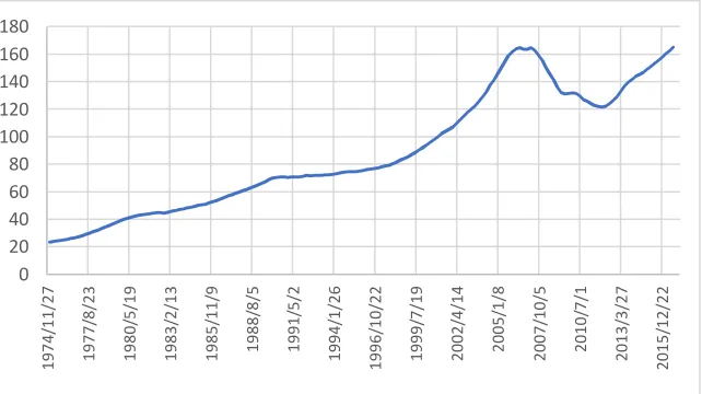
the financial effect. In addition they have found strong evidence that fluctuations in the housing
89
1 Among the authorities were, the Fed Governors, Greenspan and Ben Bernanke.
2 We could’ve included the effect of TRA 1986 in the whole sample with the use of dummy variables, but we
market wealth have a significant impact on consumption. This key finding was robust to various
90
techniques used. Benjamin et al. (2003), with the use of U.S. state-level data, reports sizable housing
91
wealth effects, a result that is in line with the ones obtained by CQS. They also reported that the
92
marginal propensity to consume from housing wealth is significant and higher than that of financial
93
wealth. In the same vein, Bostic, Gabriel, and Painter (2009) utilizing data from the Survey of
94
Consumer Finances and the Consumer Expenditure Survey, for the period of 1989 to 2001 argue for
95
relatively larger housing wealth effects (with an estimated elasticity of 0.06) in comparison with
96
financial wealth (estimated elasticity 0.02).
97
On the other side, Elliot (1980) conducted an early study of the impact of non-financial and
98
financial wealth on consumption spending using aggregate data, and concluded that non-financial
99
wealth had no impact on consumption. Dvornak and Kohler (2003) obtained opposite results in
100
application of the CQS methodology to the Australian economy, with larger and significant financial
101
wealth effects, than the effects of housing wealth. Attanasio et al. (2009) employing micro-level
102
data for England concluded that there was no housing wealth effect on consumption.
103
Calomiris et al. (2009), re-examine the impact of housing wealth, by employing the CQS data.
104
Following a method suggested by Hall (1978), Auerbach and Hassett (1989) and Campbell and
105
Mankiw (1990), they find that the estimated housing wealth has much smaller magnitude and less
106
significant effect on consumption, compared with the financial wealth effect. This comes in direct
107
contrast with the results obtained by CQS. In fact, the coefficient of the financial wealth ranges
108
between 0.149–0.230, while the coefficient of housing wealth is between 0.024–0.065. Moreover the
109
income coefficient fall within the 0.3–0.7 range, in agreement with the ones found by Campbell and
110
Mankiw (1990). However, Calomiris et al. (2013) extend their previous model by considering the
111
role of age composition and wealth distribution. By constructing new panel data they find that the
112
effect of housing wealth on consumer spending depends crucially on age composition, poverty rates,
113
and the housing wealth share. They support that consumers with different age and wealth
114
characteristics have different housing wealth effects especially due to credit constraints. Generally,
115
housing wealth effects are higher in state-years with higher housing wealth shares.
116
De Bonis and Silvestrini (2012), by using panel data for a number of OECD countries also found
117
greater impact on financial asset than the actual effects of housing wealth on consumption.
118
Recently, since special attention was paid to the role of lending collateral real estate Cooper
119
(forthcoming) finds slightly greater effect of financial wealth from the effects of real estate.
120
Sierminska and Takhtamanova (2012) showed that the relative magnitude of the effect of financial
121
wealth against the effect of real estate depends on the country to be studied and that differences
122
within countries can be guided by certain age groups. Phang (2004) supports this argument by
123
showing that an increase in housing price has no significant effect on aggregate consumption in
124
Singapore.
125
In terms of long-run relationship and applying an error correction framework, Belsky and
126
Prakken (2004) find that the estimated consumption effects of real estate and corporate equity are
127
sizable and similar in magnitude (about 51/2 cents on the dollar), but different in immediacy of
128
impact. As follows, Bampinas et al. (2017) examine the role of inequality and demographics.
129
Based on the same model specification and data from CQS, and employing quantile regression
130
techniques, they find first, that at the lower end of the conditional distribution of consumption the
131
two types of wealth are statistically significant and of similar size (0.053-0.088).
132
Demographics are not significant, while the effect of income inequality as measured by the Gini
133
coefficient at the state level is negative and significant. As they move to higher quantiles, the effect
134
of income and housing wealth is increasing and the effect of financial wealth is decreasing. At
135
higher quantiles the coefficient of housing wealth is at least two times that of financial. They also
136
find that a larger percentage of people over 65 years of age and a higher degree of income inequality
137
also lead to lower consumption in the long-run.
138
Furthermore, since private consumption historically represents about 70 percent of US-GDP,
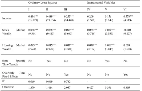
139
based on search query time series provided by Google Trends. The results suggest that Google
141
Trends may be a new source of data to forecast private consumption.
142
Lahiri et al. (2015) introduce consumer confidence to forecast consumption and employ
143
real-time data. The consumer confidence was based on a survey, which tracked many different
144
aspects of consumer attitudes and expectations about economy. The results show that consumer
145
confidence has a notable and positive contribution in forecasting personal consumption
146
expenditure. Dees and Soares Brinca (2011) investigate the role of confidence for forecasting
147
consumption change in USA and Europe. They found that it brings additional information beyond
148
to income, wealth, interest rates etc. Generally, expectations can be in certain circumstances a good
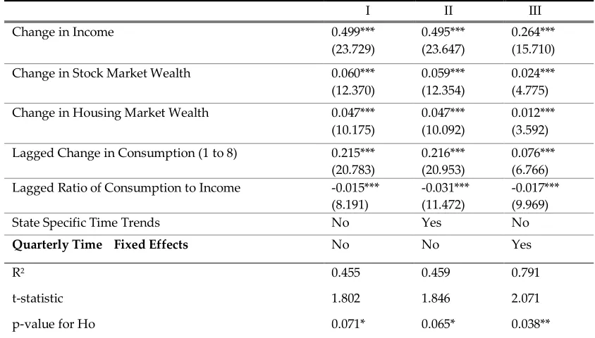
149
predictor of consumption, additionally to income and wealth.
150
3. Data and Methodology
151
3.1. Data
152
This section provides a summary description of the data used in our analysis. A more detailed
153
description can be found in the Appendix A. The data are quarterly in frequency and span from
154
1975 (1st quarter) to 2016. All variables are in chained 2005 dollars, measured per capita in
155
logarithms, and seasonally adjusted by census X12.
156
We use state-level panel data in order to get more accurate estimates especially for the two
157
wealth variables, and, at the same time, to allow us in getting significance and probably differences
158
in magnitude. The employed variables are consumption, personal income, financial wealth and
159
housing wealth. We use retail sales as proxy for consumption. In order to obtain retail sales for
160
each State, unlike CQS who got the data from Moody’s Economy.com, we get from Bureau of
161
Economic Analysis (BEA) national quarterly retail sales data as well as state-level retail trade data.
162
Next, the percentage share of the retail trade data for each State is allocated to the national retail
163
sales data in order to obtain the State-level retail sales. For personal income data are taken from
164
Bureau of Economic Analysis converted in to real per capita personal income. For total financial
165
wealth we obtained the data from the Federal Reserve Flow of Funds calculated as the sum of
166
corporate equities, mutual fund shares and pension fund. Then, on a state-level data, from BEA we
167
subtract the “Private nonfarm earnings Real estate” from “Private nonfarm earnings finance,
168
insurance and real estate” in order to get net earnings finance and insurance.
169
We finally, allocate that measure of National aggregate financial wealth among states based on
170
the share of Private nonfarm earnings, Finance and Insurance.
171
Lastly, we obtain date from Census of Population and Housing in order to calculate the housing
172
wealth for each state. For the construction of this variable the CQS procedure was utilized, but the
173
number of households per state and the weighted repeat sales price index were calculated
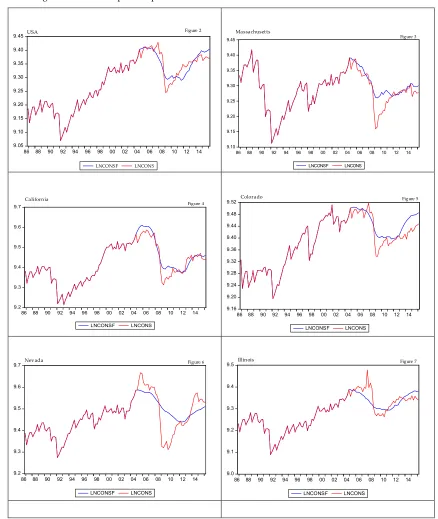
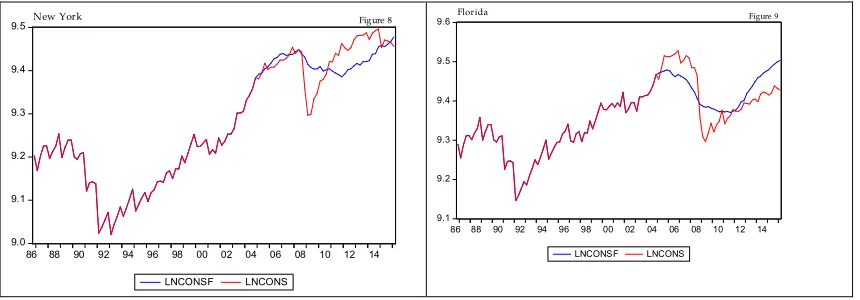
174
differently. Detailed description of constructing the variables is provided in the Appendix.
175
Before we begin with the methodology it is important to depict the performance of the housing
176
and the financial wealth for the time period under investigation. Fig. 1 reports the two national
177
measures of house and financial wealth from 1975 to 2016. It seems that the housing wealth never
178
declines from 1975 to 2007. Even for the period where the DotCom crisis greatly impacted the
179
financial wealth and consequently the Economy (March 2000), the housing wealth continues to rise
180
182
Figure 1. Financial and housing wealth in USA, during the period 1975-2016, (in billion of US
183
dollars).
184
3.2. Methodology
185
In this section we start our analysis by investigating if the variables are stationary. Based on
186
two different methods namely a) the Im, Pesaran and Shin W-stat, and, (b) PP- Fisher chi-square we
187
estimate the unit root hypothesis for consumption, income, financial wealth and housing wealth.
188
Tests assume a null hypothesis of joint stationarity against the null that all series are non-stationary.
189
Under cross-sectional independence, each of these statistics is distributed as standard normal as
190
both N (states) and T (time) increasing. Table 1 presents the results of the panel unit root tests with
191
intercept and intercept and trend. The analysis shows that all variables are stationary at the 5%
192
significance level of the first difference, meaning that all variables are I (1) processes. Although the
193
next step is to test for the long run relationship and possible cointegration, we follow the CQS
194
method; regressing the difference of consumption on the differences of income, financial and
195
housing wealth. While this specification addresses the nonstationarity issue, we understand that it
196
does not take into account possible cointegration relationship. But we proceed in order to compare
197
our results with the ones obtained by CQS, Calomiris et al. (2009, 2013) and Bampinas et al. (2017).
198
Table 1. Results for panel unit root tests.
199
IPS PP – Fisher Chi-square
Variable Constant Constant trend Constant Constant trend
lnConsumption -0.78[0.2179] -6.42 [0.0000] 138.05[0.0101] 202.79[0.0000] lnIncome 0.29[0.6157] 2.67[0.9962] 82.73[0.9188] 59.72[0.9999] lnFinancialWealth 8.65[1.0000] -1.63[0.0511] 17.030[1.0000] 112.96[0.2154] lnHousingWeatlh 2.46[0.9931] -5.43[0.0000] 66.24[0.9977] 274.82[0.0000] ΔlnConsumption -24.26[0.0000] -81.68[0.0000] 4194.05[0.0000] 5107.04[0.0000]
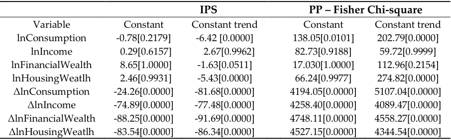
ΔlnIncome -74.89[0.0000] -77.48[0.0000] 4258.40[0.0000] 4089.47[0.0000] ΔlnFinancialWealth -88.25[0.0000] -91.69[0.0000] 4748.11[0.0000] 4558.27[0.0000] ΔlnHousingWeatlh -83.54[0.0000] -86.34[0.0000] 4527.15[0.0000] 4344.54[0.0000]
Ln is the natural log and Δ is the first difference operator. Numbers in brackets are p-values. The
200
maximum lag length is set to 6, determined by the Schwarz Bayesian Criterion.
201
0 10,000 20,000 30,000 40,000 50,000
1975 1980 1985 1990 1995 2000 2005 2010 2015
FINANCIAL W EALTH USA HOUSING W EALTH USA
The estimated equation is given as:
202
t it
it it
it
Y
FW
HW
FEffects
e
C
1
3 (1)The equation shows the relationship between consumption (C), personal income (Y), stock (FW)
203
and housing wealth (HW). We test three different specification models with the variables to be in
204
first differences. Model I, II and III are the basic specifications representing the effects of changes in
205
both housing and stock-market wealth upon consumption. Model II explores further the nature of
206
estimated wealth effects and their robustness by including state-specific time trends, while model III
207
includes time fixed effects. Please note that the above model specifications, as articulated by
208
Calomiris et al. (2009), lead to inconsistent results, since the residual contains changes in permanent
209
and current income and these will likely be highly correlated with changes in housing and stock
210
wealth. In order to correct for any correlation issues, we proceed with the estimation of three other
211
models IV, V and VI with the use of two-stage least squares and instrumental variables3. As
212
instruments we use lagged variables of income changes, housing wealth changes and stock market
213
changes. The hypothesis that the housing market wealth parameter is equal to the stock market
214
wealth parameter is tested by the Wald test coefficient restriction.
215
As a next step we use the following error correction model (ECM)4,5 utilized by CQS. We
216
understand that the basic format given by Brooks (2008), as given by eq. 2 differs from the one
217
presented by CQS, eq. 3 in a number of ways:
218
y
x
error
x
y
t
t
t
t
1
2 1
1 (2)t t t
t t
t t
t
C
Inc
FW
HW
C
Inc
C
1 1 2 3[
1 1]
(3)Firstly, CQS estimates eq. 3 by including lags of consumption, in order to correct for
219
autocorrelation. Secondly, for the parameter γ, in eq. 2, which measures the speed of adjustment
220
back to equilibrium and the long-term relationship between income and consumption, CQS
221
impose-without estimation – a cointegrating vector with a parameter of one.
222
Finally, given the original model (1), we are building the model for predicting consumption as
223
follows. We construct our model in time series for USA and the 8 States except District of Columbia
224
in order to use it for forecasting the consumption change. We forecast the consumption of
225
Massachusetts, Illinois, Colorado, Nevada, California, Florida, New York and USA. The equation
226
specification consists of the dependent variable of consumption (in logs) followed by the list of
227
regressors, we used in this paper (the income and the two types of wealth). We include
228
consumption with one lag as independent variable for forecasting purposes (because the dependent
229
variable is an auto-series). The estimated equation is:
230
231
t t t
t t
t
C
Inc
FW
HW
C
log
log
log
log
log
1 1 2 3 (4)3 The instrumental variables version takes account of possible endogeneity problems
4 Carrol et al. (2011) argue that cointegration methods are problematic for estimating wealth effects, for at least
two reasons. First, basic consumption theory does not imply the existence of a stable cointegrating vector; in particular, a change in the long-run growth rate or the long-run interest rate should change the relationship between consumption, income, and wealth. Second, even if changes to the cointegrating vector are ruled out by assumption, changes in any other feature of the economy relevant for the consumption/saving decision can generate such long-lasting dynamics that hundreds or thousands of years of data should be required to obtain reliable estimates of that vector.
5 Instead of ECM estimation the literature suggests fixed-effect estimator procedure, dynamic OLS, mean
We use the model to forecast future values of consumption which we have already estimated.
232
In fact we know the real values of consumption. Initially, we determime whether the forecast is
233
accurate or not, which would then be compared with the actual values, and the difference between
234
them. Therefore, we use the same set of data that was used to estimate the model’s parameters
235
(in-sample forecasts) to see how well our model performs out-of-sample.
236
We first estimate the model using data from 1986 fourth quarter to 2016 first quarter. Then we
237
conduct in-sample forecasts from the first quarter of 2005 until the first quarter of 2016, using a
238
lagged dependent variable according the information criteria. We construct dynamic forecast to
239
calculate multi-step forecasts starting from the first period in the forecast sample.
240
3.3. The Tax Reform Act of 1986
241
Following we take in consideration the Tax Reform Act enacted in October 1986 (TRA, 86).
242
The TRA (86) among other encourages certain types of investments. It was a tax-simplification Act
243
and chopped the top individual income tax rate from 50% to 28% while curbing special deductions,
244
exclusions and breaks, such as tax expenditures (Novack 2011). The Act also increased incentives
245
favoring investment in owner-occupied housing, by increasing the home mortgage interest
246
deduction. We proceed with re-estimating the model over the time period from 1986 to 2016. We
247
understand that the two classes of wealth may have differences in terms of liquidity, with the
248
housing to be less liquid since it is impossible to liquidate just a part of it. Furthermore one should
249
take into account the high processed fees for doing that. But since the end of 1986, home owners
250
had the ability for home equity loans, refinancing with better terms and thus have more spending
251
income for consumption.
252
3.4. The Case-Shiller Metropolitan areas Index
253
As a last step we perform the same analysis for the 10 metropolitan areas given by the Case
254
Shiller composite 10 index6. We first depict in fig. 2 the index from 1974 until the end of 2016, to see
255
the evolution of the house prices through time. One could easily notice the positive trend displayed
256
from 1974 until 2007. But the prevalent increase of the index occurred between 2002 and 2007,
257
where ample market liquidity and lax credit conditions drove the house prices much higher, across
258
the United States. From 2007 until the end of the 3th quarter of 2011, the house prices decrease
259
significantly before start increasing again.
260
261
Figure 2. House price Index for 10 U.S. Metropolitan areas (Case-Shiller Composite 10) (2000=100).
262
6 The metropolitan areas are: Greater Boston, Chicago metropolitan area, Denver-Aurora Metropolitan Area,
Las Vegas metropolitan area, Greater Los Angeles, South Florida metropolitan area, New York metropolitan area, San Diego County, San Francisco and Washington Metropolitan Area.
Testing the specific metropolitan areas comes from the notion that there might be distributional
263
factors at work (Dvornak and Kohler 2007). In other words, uneven distribution of wealth is very
264
pronounced, and, although housing is held by a great majority of households, regardless of income
265
classes, stock market wealth is held largely by the higher-income class. Indeed, this is more evident
266
in other developed countries, but there is a notion that high-income class propensity to consume out
267
of income and stock wealth is lower, pertaining that changes in housing wealth might have a larger
268
effect on consumption. As Carroll (2012) reports the 20% of U.S. households hold most of the
269
country’s overall net worth. Also, a good reason for testing the wealth effect on the particular
270
metropolitan areas, as CQS pointed out, is the fact that home prices have evolved very differently in
271
different parts of the country, and therefore can be substantial differences in the elasticity of land
272
supply, the performance of State economies, and their changing demographics.
273
Since there is no data available for the U.S. 10 metropolitan areas, we utilize the associated
274
State-based data. For that reason, we test the wealth effect on consumption of the 8 States where
275
the metropolitan areas are part of them. In particular the States are Massachusetts, Illinois,
276
Colorado, Nevada, California, Florida, New York and District of Columbia.
277
4. Results and Discussion
278
Table 2 depicts the results of all six models. The first observation is that consumption changes
279
are significantly dependent on changes in income and in both forms of wealth. But in all
280
specifications, stock market wealth has a positive and greater effect on consumption compared to the
281
housing wealth effect. For models I and II, the stock market effect is 0.058 while for the housing
282
effect the parameter is equal to 0.045. Both parameters appear to be statistically significant at 1%
283
level. Interesting enough, the sum of the financial and housing estimated parameters is almost equal
284
to the sum obtained by CQS. Also, the estimated income effect on consumption is equal to around
285
0.49, which is within the 0.3-0.7 range found by Campbell and Mankiw (1990).
286
Table 2. Consumption Models in first differences. Panel data from 1975 to 2016.
287
Dependent variable: Change in Consumption per capita
Ordinary Least Squares Instrumental Variables
I II III IV V VI
Income 0.494*** (19.271)
0.489*** (19.034)
0.233*** (14.478)
0.209 (1.571)
0.156 (1.149)
0.378*** (4.513)
Stock Market Wealth
0.058*** (9.364)
0.058*** (9.413)
0.029*** (5.662)
0.085*** (3.716)
0.081*** (3.553)
-0.010 (0.227)
Housing Market Wealth
0.045*** (7.670)
0.045*** (7.624)
0.011*** (3.381)
0.070*** (3.177)
0.068*** (3.048)
0.018 (1.603)
State Specific Time Trends
No Yes No No Yes No
Quarterly Time
Fixed Effects No No Yes No No Yes
R2
0.069 0.069 0.782 - - -
p-value for Ho 0.168 0.149 0.003 0.669 0.696 0.545
Note: Ho is the test of the hypothesis that the coefficient on housing market is equal to that of stock market; t-statistics are in parentheses and ***, **,* are estimated value significant at the 1%, 5% and 10% level respectively.
The importance of the stock market wealth on consumption is reinforced by the results derived
288
from model III which includes fixed effects, and by models IV and V, where changes in stock market
289
wealth have still greater impact, than the housing effect on changes in consumption. The results are
290
in direct contrast to the findings of CQS, but in an agreement with Calomiris et al. (2009). Also,
291
table 2 reports the t statistics for the hypothesis that the coefficient of stock market wealth is equal to
292
the coefficient of the housing-market wealth. The results suggest that we could not reject the
293
hypothesis that that financial wealth could be equal in importance to the housing wealth. Only in
294
model III, the financial wealth is greater and more important than the housing wealth.
295
Table 3 presents the results of the error correction model and support the highly significant
296
immediate effect of financial wealth on consumption, as well as the housing effect. But the financial
297
wealth coefficient is larger in magnitude than the housing coefficient. For I and II models the
298
financial coefficient takes a value of around 0.062, while for the housing parameter is 0.047. In the
299
third model when fixed effects are included the estimated parameters decrease in magnitude but
300
still the financial wealth appears to be greater and more significant than the housing wealth effect.
301
Furthermore, the results obtained by ECM are consistent with the results found by the first
302
difference model specification. As for the lagged ratio of consumption to income, the coefficient is
303
negative and significant in both cases, reviling an immediate correction of the potential shocks. It
304
also suggests that transitory shocks, arising from changes in other variables in the model or in the
305
error term, will have an immediate effect on consumption. This effect will eventually be offset,
306
unless the shock is ultimately confirmed by income changes (CQS 2012).
307
Table 3. Error Correction Consumption Models. Panel data from 1975 to 2016.
308
Dependent variable: Change in Consumption per capita
I II III
Change in Income 0.499***
(23.729)
0.495*** (23.647)
0.264*** (15.710)
Change in Stock Market Wealth 0.060***
(12.370)
0.059*** (12.354)
0.024*** (4.775)
Change in Housing Market Wealth 0.047***
(10.175)
0.047*** (10.092)
0.012*** (3.592) Lagged Change in Consumption (1 to 8) 0.215***
(20.783)
0.216*** (20.953)
0.076*** (6.766) Lagged Ratio of Consumption to Income -0.015***
(8.191)
-0.031*** (11.472)
-0.017*** (9.969)
State Specific Time Trends No Yes No
Quarterly Time Fixed Effects No No Yes
R2 0.455 0.459 0.791
t-statistic 1.802 1.846 2.071
p-value for Ho 0.071* 0.065* 0.038**
In Table 4 we repeat the same methodology and present only the estimates of the error
309
correction models, with the sample data spanning from end 1986 until 2016. The results support
310
again the highly significant immediate effect of financial wealth on consumption, which is more than
311
2 cents higher than the effect of housing wealth. Surprisingly, we find that the housing effect is
312
lower than before, irrespective of the estimation method chosen. The opposite is reported for the
313
financial wealth where the effect on consumption is now 0.066 to 0.068 instead of 0.060. It is worth
314
pointing out the increase, in absolute terms, of the estimated parameter measuring the lagged ratio
315
of consumption to income, reviling again a very immediate correction of the any potential shocks.
316
In concluding, based on the error correction estimates the 1986 Act seems not to change people
317
preferences and still the financial wealth effect is greater and significantly more important, based on
318
the Wald test, than the housing wealth effect on consumption.
319
Table 4. Error Correction Consumption Models for the period 1987-2016, after the introduction of
320
the Tax Reform Act in 1986.
321
Dependent variable: Change in Consumption per capita
I II III
Change in Income 0.532***
(19.093)
0.528*** (19.025)
0.425*** (17.376) Change in Stock Market Wealth 0.068***
(13.257)
0.066*** (12.952)
0.010** (1.748)
Change in Housing Market Wealth 0.042*** (8.331)
0.042*** (8.361)
0.009*** (2.857)
Lagged Change in Consumption (1 to 8) 0.208*** (17.249)
0.211*** (17.562)
0.042*** (3.219)
Lagged Ratio of Consumption to Income -0.035*** (11.362)
-0.057*** (13.753)
-0.037*** (12.754)
State Specific Time Trends No Yes No
Quarterly Time Fixed Effects No No Yes
R2 0.313 0.321 0.713
t-statistics 15.768 15.798 6.156
p-value for Ho 0.000 0.000 0.000
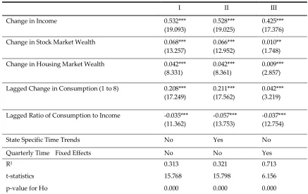
Note: Ho is the test of the hypothesis that the coefficient on housing market is equal to that of stock market; t-statistics are in parentheses and ***, **, * are estimated value significant at the 1%, 5% and 10% level respectively.
Table 5 presents the results of the first three specification models, where the variables are in
322
first differences, along with the error correction models, in an attempt to test the consistency of the
323
estimated parameters. The results are surprisingly different now and in direct contrast to the
324
findings of the previous sections of the paper. Now, the estimated housing effect is larger in
325
magnitude and more significant than the financial wealth effect. The MPC out of housing wealth is
326
in the region of 0.052 while the MPC for stock wealth is around 0.021. In most of the cases, the stock
327
wealth estimate is not even statistically significant. In addition the estimated income coefficient is
328
much greater in magnitude and steadily in the area of 0.59 compared with only 0.49 before, and still
329
within the 0.3–0.7 range estimated by Cambell and Mankiw (1990). The results from the first three
330
models are supported by the error correction estimates depicted by the models IV, V and VI in table
331
5. The estimates of the housing wealth parameter are more than double in magnitude than the
332
once more very small, indicating the immediate restoration of consumption after a shock in the
334
residuals in the short run.
335
Table 5. OLS Model for Consumption and Error Correction for the period 1987-2016, for the 8
336
States, after the introduction of the Tax Reform Act in 1986.
337
Dependent variable: Change in Consumption per capita
Ordinary Least Squares Error Correction Model
I II III IV V VI Change in Income 0.583***
(6.131)
0.589*** (6.189)
0.549*** (5.832)
0.599*** (6.565)
0.594*** (6.517)
0.605*** (6.062) Change in Stock
Market Wealth
0.021 (1.225)
0.022 (1.278)
0.004 (0.272)
0.030* (1.862)
0.029* (1.820)
0.002 (0.132) Change in Housing
Market Wealth
0.052*** (3.203)
0.051*** (3.183)
0.022* (1.873)
0.055*** (3.748)
0.055*** (3.747)
0.024** (2.018) Lagged Change in
Consumption (1to8 lags)
- - - 0.205***
(6.525)
0.207*** (6.613)
0.103*** (2.884)
Lagged Ratio of Consumption to Income
- - - -0.032***
(4.888)
-0.044*** (5.051)
-0.029*** (4.410)
State Specific Time Trends
No Yes No No Yes No
Quarterly Time Fixed Effects
No No Yes No No Yes
R2 0.061 0.063 0.681 0.269 0.272 0.688
t-statistic 1.261 1.210 0.873 1.122 1.151 1.063
p-value for Ho 0.208 0.227 0.383 0.262 0.250 0.288
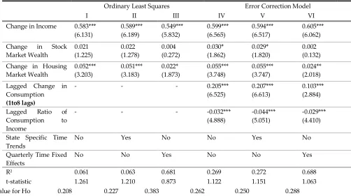
Note: Ho is the test of the hypothesis that the coefficient on housing market is equal to that of stock market; t-statistics are in parentheses and ***, **, * are estimated value significant at the 1%, 5% and 10% level respectively.
338
4.1. Forecasting the consumption change
339
Table 6 compares the forecasted (predicted) values from the model (over the period 2005q1 to
340
2016q1) to the actual data and computes the forecast evaluation table (6).
341
Table 6. Forecast evaluation table
342
The forecast statistics for the 7 States comprised the Case-Shiller Index and US.
States RMSE MAE Theil
Inequality Coefficient
Bias Variance Variance Proportion
Massachusetts 0.0344 0.0233 0.0018 0.3492 0.1775
Ilinois 0.0366 0.0277 0.0019 0.0234 0.1433
Colorado 0.0321 0.0261 0.0017 0.4354 0.0724
Nevada 0.0751 0.0558 0.0039 0.0193 0.5268
California 0.0339 0.0268 0.0017 0.2390 0.0000
Florida 0.0473 0.0419 0.0025 0.0656 0.2353
USA 0.0262 0.0213 0.0014 0.0011 0.0132
The root mean squared error is about 0.02-0.07 and the mean absolute error ranges from
343
0.02-0.04. Bias proportion is about 0.00-0.43, while the variance proportion is about 0.01-0.31.
344
The reported forecast statistics indicate that our forecasting model perform well out-of-sample.
345
Figures 2-10 display the results of forecasting consumption change in Massachusetts, Illinois,
346
Colorado, Nevada, California, Florida, New York and USA.
347
Figure 2-10. Consumption in predicted and actual values
348
9.05 9.10 9.15 9.20 9.25 9.30 9.35 9.40 9.45
86 88 90 92 94 96 98 00 02 04 06 08 10 12 14
LNCONS F LNCONS
USA Figure 2
9.10 9.15 9.20 9.25 9.30 9.35 9.40 9.45
86 88 90 92 94 96 98 00 02 04 06 08 10 12 14
LNCONSF LNCONS
Massachuset ts
Figure 3
9.2 9.3 9.4 9.5 9.6 9.7
86 88 90 92 94 96 98 00 02 04 06 08 10 12 14
LNCONSF LNCONS
California
Figure 4
9.16 9.20 9.24 9.28 9.32 9.36 9.40 9.44 9.48 9.52
86 88 90 92 94 96 98 00 02 04 06 08 10 12 14 LNCONSF LNCONS
Colorado Figure 5
9.2 9.3 9.4 9.5 9.6 9.7
86 88 90 92 94 96 98 00 02 04 06 08 10 12 14 LNCONSF LNCONS
Nevada Figure 6
9.0 9.1 9.2 9.3 9.4 9.5
86 88 90 92 94 96 98 00 02 04 06 08 10 12 14 LNCONSF LNCONS
9.0 9.1 9.2 9.3 9.4 9.5
86 88 90 92 94 96 98 00 02 04 06 08 10 12 14 LNCONSF LNCONS
New York Figure 8
9.1 9.2 9.3 9.4 9.5 9.6
86 88 90 92 94 96 98 00 02 04 06 08 10 12 14 LNCONSF LNCONS
Florida Figure 9
349
We conclude that the big dip in consumption in 2008 was not predicted in any state, as well as
350
the large rise in consumption for 2005. Generally, extreme consumption behaviors were not
351
predictable. Our panel results show that the effect of housing wealth is larger on consumption
352
compared to financial wealth. Simultaneously, literature evidence (Attanasio O. et.al, 2009) finds
353
that the relationship between house prices and consumption is stronger for younger than older
354
households. The young are more vulnerable in irrational behaviors and more likely to be
355
credit-constrained and thus willing to borrow against any increase in housing equity.
356
Furthermore, while the forecast showed a recession from 2008 to the last quarter of 2011, in fact
357
from the first quarter of 2009 the economy in America began to recover in all States, probably due to
358
quantitative easing, which was started in November 2008. The Fed increased the amount of money
359
by going to the financial markets to buy assets and generating new money to pay for it. Specially,
360
in N. York and Nevada the real consumption exceeds forecasts.
361
5. Conclusion
362
We have followed Case et al. (2012) in an attempt to estimate the effect of changes in financial
363
and housing wealth on change in household consumption for the time period of 1975 to 2016.
364
Constructing the housing and finance data differently from the method used Case et al. (2012) we
365
find first that both financial and housing wealth are significant determinants of household
366
consumption and secondly the effect of the financial wealth is larger in magnitude from the housing
367
wealth effect. For most of model specifications a 1 $ change in stock market wealth will change
368
consumption by 5.8 – 6 cents, whereas in terms of housing wealth consumption will increase by only
369
4.5 – 4.7 cents. Our panel results are in contrast to CQS studies and in line with the ones obtained
370
by Calomiris et al. (2009). But when we test the top 10 metropolitan areas due to the fact that
371
distributional factors could be at work and the that home prices have evolved very differently in
372
different parts of the country, meaning substantial differences in the elasticity of land supply, we
373
find that the estimate housing wealth has greater and robust effect on consumption than the stock
374
market wealth. The difference with the CQS results could be explained because we use mainly an
375
alternative methodology for measuring of stock market and housing wealth. Therefore, we could
376
agree with Calomiris et al. (2013) that the results are very sensitive with the choice of housing wealth
377
measure.
378
Finally, we forecast consumption change in the 7 states that include the 10 (richer) Metropolitan
379
areas comprising of the well known Case-Shiller 10-City Composite Index and the USA. We
380
conclude that our model is a good predictor and extreme behaviors in consumption were not
381
predictable. Additionally, while the forecast showed a recession from 2008 to the last quarter of
382
2011, in fact from the first quarter of 2009 the economy in America began to recover. The main reason
383
may be the aggressive monetary policy followed and the quantitative easing that has spurred
384
consumption. However, expectations for greater consumption were not verified for most areas.
Data Appendix.
389
Consumption
390
There are no direct measurements of U.S. consumption for each state separately, thus, CQS
391
used a panel of retail sales (as a proxy), which has been constructed by Moody’s Economy.com
392
(Formerly Regional Financial Associates, RFA. See Zandi, 1997). “The RFA estimates were
393
constructed from county level sales tax data, the Census of Retail Trade published by the U.S.
394
Census Bureau, and the Census Bureau’s monthly national retail sales estimates. For states with no
395
retail sales tax or where data were insufficient to support imputations, RFA based its estimates on
396
the historical relationship between retail sales and retail employment.
397
We followed a different way in obtaining retail sales. We obtain the aggregate quarterly retail
398
sales for the whole economy and the retail trade of the 51 states from
399
http://www2.census.gov/retail/releases/ and www.bea.gov. Then the aggregate retail sales are
400
allocated across states based on the distribution of retail trade across states. Our data were
401
consistent without any empty intervals.
402
Financial Wealth
403
Estimates of the accumulated financial wealth in U.S. per quarter have been obtained according
404
to the detailed instructions of CQS (2005, 2013) from the Federal Reserve Flow of Funds (FOF)
405
accounts for every quarter. We computed (from FOF) the sum of mutual funds, corporate equities
406
and pension fund reserves that are held by the household sector.
407
The allocation of the aggregate financial wealth across states was done the data taken from The
408
Bureau of Economic Analysis (BEA) and namely the two categories, a) “Private nonfarm earnings
409
real estate” and b) “Private nonfarm earnings, finance, insurance and real estate”. By subtracting a)
410
from b) we got the private nonfarm earnings, finance and insurance. Then the distribution of this
411
outcome used to allocate the aggregate financial wealth across states.
412
On the other hand CQS allocated aggregate financial wealth based on data furnished by the
413
Investment Company Institute (ICI) which were available only for 1986, 1987, 1989, 1991 and1993.
414
For the interval 1993 to 2009, CQS interpolated the share of holdings in each state, linearly, mapping
415
the 1993 figures to the 2008 figures.
416
Housing wealth
417
CQS constructed the panel of aggregate housing wealth data for each state through the
418
following equation:
419
io it it it
it
R
N
I
V
V
420
where,
421
1.
V
it: aggregate of owner occupied housing in state i in quarter t,422
2.
R
it: homeownership rate in state i in quarter t,423
3.
N
it: number of households in state i in quarter t,424
4.
I
it: weighted repeat sales price index, for state i in quarter t, and,425
Our differences with the data used by CQS are in the third and fourth dataset. For the
427
number of households in state i in quarter t, we used the data from CENSUS
428
https://www.census.gov/hhes/families/files/hh4.csv
429
https://www.census.gov/popest/research/p25-1123.pdf and in particular the proportion of the
430
population for each state which was used as a proxy for the number of households per state. We
431
compare the outcome of this procedure with the data provided by Statistical Abstract of USA, (we
432
did not use the Statistical Abstract of USA in the first place since the figures where different from
433
issue to issue). Regarding the fourth category, about the house prices, we used the Median Sales
434
Price of Houses Sold for each region and applied the percentage change in median home value in
435
1970 which we had at our disposal for each state.
436
As for the index of repeat sales (price index), we used data from Freddie May Housing Price
437
Index (FMHPI),
438
https://www.quandl.com/data/FMAC/HPI-House-Price-Index-All-States-and-US-National. The
439
series are available at a state-level, and the and begin in January 1975. The FMHPI is based on an
440
ever-expanding database of loans purchased by either Freddie Mac or Fannie Mae.
441
Personal income
442
The quarterly data are from the Bureau of Economic Analysis (2016Q4 release).
443
References
444
1. Ando, A.; Modigliani, F. The Life Cycle Hypothesis of Saving: Aggregate Implications and Tests. The
445
American Economic Review 1963, 53, 55-84, URL: 1817129.
446
2. Attanasio, P.O.; Blow, L., Hamilton, R.; Leicester, A. Booms and Busts: Consumption, House Prices and
447
Expectations. Economica 2009, 76, 20-50, doi:10.1111/14680335.
448
3. Auerbach, J. A.; Hassett, Κ. Corporate Savings and Shareholder Consumption 1989, NBER Working
449
Paper No. 2994.
450
4. Bampinas, G.; Konstantinou, P.; Panagiotidis, Τ. Inequality, Demographics and the Housing Wealth
451
Effect: Panel Quantile Regression Evidence for the US. Finance Research Letters 2017, 23, 19-22,
452
Doi:10.1016/j.frl.2017.01.001.
453
5. Belsky E.; Prakken, J. Housing Wealth Effects: Housing’s Impact on Wealth Accumulation, Wealth
454
Distribution and Consumer Spending. 2004,National Center for Real Estate Research 2004, Joint Center for
455
Housing Studies of Harvard University.
456
6. Benjamin, J.; Chinloy, P.; and Jud, D. Why do Households Concentrate Their Wealth in Housing? Journal of
457
Real Estate Research 2004, 26(4), 329-344.
458
7. Bonis, De R.; Silvestrini, A. The effects of financial and real wealth on consumption: new evidence from
459
OECD countries. Applied Financial Economics 2012, 22(5), 409-425.
460
8. Bostic, R.; Stuart, G.; Gary, P. Housing wealth, financial wealth, and consumption: New evidence from
461
micro data. Regional Science and Urban Economics 2009, 39(1).
462
9. Brooks, C. Introductory Econometrics for Finance, 2nd Ed. Cambridge University Press: New York, NY,
463
USA, 2008, ISBN-13 978-0-511-39848-3.
464
10. Buiter, H. W. Housing Wealth Isn’t Wealth. Economics: The Open-Access. Open Assessment E-Journal 2010,
465
4, 2010-22.
466
11. Calomiris, C.; Longhofer, S. D.; Miles, W. The (Mythical?) Housing Wealth Effect 2009. NBER Working
467
Paper No 15075.
468
12. Calomiris, C.; Longhofer, S. D.; Miles, W. The housing wealth effect: the crucial roles of demographics,
469
wealth distribution and wealth shares. Crit. Finance Rev. 2013, 2, 49-99, Doi:10.1561/104.00000008.
470
13. Campbell, J.; Mankiw, G. The Response of Consumption to Income. European Economic Review 1991, 35,
471
723-767.
472
14. Carroll, D.C.; Otsuka, M.; Slacalek, J. How Large are Housing and Financial Wealth Effects? A New
473
Approach. Journal of Money, Credit and Banking 2011, 43, 55-79.
474
15. Case, K. E.; Quigley, J. M.; Shiller, J. R. Comparing Wealth Effects: The Stock Market versus the Housing
475
16. Case, K. E.; Quigley, J. M.; Shiller, J. R. Wealth Effects Revisited 1978-2009. COWLES FOUNDATION
477
Discussion Paper No. 1784, 2011, Yale University, New Haven, Connecticut 06520-8281.
478
17. Case, K. E.; Quigley, J. M.; Shiller, J. R. Wealth Effects Revisited 1975-2012. Critical Finance review 2012, 2,
479
101-128, Doi:10.1561/104.00000009.
480
18. Dees, S.; Soares Brinca, P. Consumer confidence as a predictor of consumption spending: evidence for the
481
United States and the euro area. ECB Working Paper 2011, No 1349, European Central Bank, Frankfurt a.
482
M., Germany.
483
19. Dvornak, N.; Kohler M. Housing Wealth, Stock Market Wealth and Consumption: A Panel Analysis for
484
Australia. Research Discussion Paper 2003-07, Reserve Bank of Australia.
485
20. Elliott, J. W. Wealth and wealth proxies in a permanent income model. Quarterly Journal of Economics 1980,
486
95, 509–535.
487
21. Hall, E. R. The Long Slump. American Economic Review 2011, 101, 431-469, Doi:10.1257/aer.101.2.431.
488
22. Lahiri, K.; Monokroussos, G.; Zhao, Y. Forecasting Consumption: the Role of Consumer Confidence in
489
Real Time with many Predictors. Journal of Applied Econometrics 2015, 31, 1254-1275, Doi:10.1002/jae.2494.
490
23. Levin, L. Are assets fungible? Testing the behavioral theory of life-cycle savings. Journal of Economic
491
Behavior & Organization 1998, 36, 59-83, Doi:10.1.1.639.4471.
492
24. Mishkin, S. F. Housing and the Monetary Transmission Mechanism. NBER Working Paper Series
493
No.13518/2007, National Bureau of Economic Research, Inc.
494
25. Novack, J. Special Report: 25 Years after Tax Reform, What Comes Next?” Personal Finance, Forbes.
495
https://www.forbes.com/sites/janetnovack/2011/10/21/. Accessed 10 November 2016.
496
26. Phang, Y. S. House Prices and Aggregate Consumption: Do they move together? Evidence from
497
Singapore. Journal of Housing Economics 2004, 13, 101-119, Doi:10.1016/2004.04.003.
498
27. Siermisnka, E.; Takhtamanova, Y. Financial and Housing Wealth and Consumption Spending:
499
Cross-Country and Age Group Comparison. Journal Housing Studies 2012, 27, 685-719,
500
Doi:10.1080/02673037.2012.697550.
501
28. Vosen, S.; Schmidt, T. Forecasting private consumption: survey-based indicators vs. Google trends. Journal
502
of Forecasting 2011, 30, 565-578, Doi:10.1002/for.1213.