R E S E A R C H
Open Access
Conditional downsampling for energy-efficient
communications in wireless sensor networks
Joan Enric Barceló-Lladó
*, Antoni Morell and Gonzalo Seco-Granados
Abstract
This paper deals with the power limitations in a wireless sensor network scenario. Concretely, we propose to use a conditional downsampling encoder (CDE) at the sensing nodes as an energy-efficient solution for the communication problem. It exploits the knowledge about the signal structure, which is assumed to be time-correlated, in order to decrease the sampling rate and hence to reduce the number of transmissions within the network. We analytically assess the performance of the CDE in terms of quadratic distortion, from which we derive closed-form expressions when it is combined with one of the two decoders: the step decoder and the predictive decoder. Moreover, we propose two methodologies to design the CDE in order to guarantee a given coding rate. We also compare the CDE, both analytically and experimentally, with other classical decimator techniques, which are the deterministic
downsampling encoder and the probabilistic downsampling encoder. Numerical simulation validates our analytical results. Moreover, we compare the obtained quadratic distortion and extract the conclusions of the capabilities of the studied encoding-decoding schemes.
1 Introduction
1.1 Motivation and previous work
Wireless sensor network (WSN) design is currently one of the most challenging topics in the communications field. In particular, WSNs are severely energy-constrained because they consist of many small, cheap, and power-limited nodes, whose batteries cannot be recharged in most cases. Hence, the application of energy-efficient algorithms turns out to be crucial.
Following with this motivation, many energy-efficient strategies can be found in order to mitigate the energy costs and hence increase the lifetime of the WSN. Without the aim of being exhaustive, we point out some examples:
• Energy-aware routing for cooperative WSNs andad hoc networks [1,2]. These techniques seek the optimum path that minimizes the total spent energy in multihop WSNs.
• Signal processing techniques for minimum-power distributed transmission schemes [3,4]. Using distributed beamforming techniques, the nodes can
*Correspondence: [email protected]
Department of Telecommunications and Systems Engineering, Universitat Autònoma de Barcelona, Bellaterra, Barcelona 08193, Spain
decrease the transmitted power at the same time that they increase the total throughput of the network. • Data-aware techniques to reduce energy by efficient
information processing [5,6]. By means of signal processing techniques, the network exploits the inherent structure and properties of the measured signal in order to sample the data and therefore reduce the associated energy costs.
Our study falls in the third category and may be com-plementary to the other approaches. Actually, we propose to encode the sensed data removing redundancy in the time domain. Many transmission schemes use non-causal transmissions such as block coding. In these cases, the source collects a number of contiguous time samples in order to compress them by removing part of (or all) the redundancy among them. Within this group of encoders-decoders, a large amount of different techniques can be found. Albeit these transmissions are very appropriate for high-rate transmissions and/or delay-tolerant communi-cations, these non-causal transmission schemes may not be applicable in some scenarios because block transmis-sions are not always allowed due to delay constraints and/or low symbol rates of the source.
For delay-sensitive applications such as real-time mon-itoring in WSNs, where the reconstruction of the signal
must take place at the same time instant as the corre-sponding input measurement, causal source codes are more convenient. Hence, a source code is said to be causal if thenth decoded sample depends on the output signal only through its first n components or, in other words, depends on the past and present outputs but not on future ones. Quantizers, delta modulators, differential pulse code modulators, and adaptive versions of these are all causal in the above sense. The basic properties of causal source codes have been introduced in 1982 in [7], and related works have been expanded so far. The work in [8] extends the general results of [7] for the case whereside information, i.e., extra information that is correlated with the source, is available at the encoder and the decoder. In addition, a causal source code is called a zero-delay or sequential code if both the encoder and the decoder are causal (note that for the causal source code definition, the assumption of causality is only at the decoder) [9,10].
In the literature, there are several zero-delay coding systems. One of the most common zero-delay coding sys-tems is the well-knowndifferential pulse code modulation (DPCM). In a nutshell, the current sample to be coded is predicted from previously coded samples. This pre-diction is used as a reference, and it is compared with the current sample. Hence, the output of the encoder is the prediction error. The inverse operation takes place at the decoder side. According to [11], DPCM was first intro-duced in a US patent by C. Cutler in 1952. Since then, many results have appeared. In particular, the autoregres-sive (AR) model has received special attention for the study of zero-delay coding schemes. Some of the early works on AR models date back to the 1960s. The works in [12,13] analyze the quadratic rate distortion of DPCM (the reader can find an extended description of the rate distor-tion in Chapter 13 of [14]). The work in [15] extends these results assuming a Gaussian distribution of the predicted error. Other works proposed algorithms for non-uniform quantizers optimized in order to minimize the distortion rate [16].
Later works, as the one in [17], try to particularize the results obtained by the DPCM also for the case of low bit rates. In such cases, the system performance becomes worse. Then, the classic DPCM encoder is modified in order to achieve better performance in terms of rate distortion for a low-bit-rate regime.
Recent works on this field have tried to unify the theoretical limits of the DPCM (and other zero-delay schemes) for AR models with other information the-ory concepts. The authors in [11] provide analyti-cal results for the existing duality between the rate distortion of an AR process with the capacity of the inter-symbol interference channels. By contrast, other works such as [9] follow an information theoretical approach that adjusts the upper and lower limits of the
rate distortion for generic zero-delay schemes using the mutual information as a measure of the achievable rate.
1.2 Our contribution
Our proposed work also follows the same sequen-tial transmission approach exposed above. Concretely, the approach of this paper is similar to that of [6], where the authors seek for the optimal sampling in a WSN scenario with correlated sources. However, we present the problem from a more realistic energy-efficient perspective. According to the results in the literature about energy consumption in sensor networks [18], the main source of energy spent in a sensor is the power dedicated to maintain the sensor awake. Con-cretely, most energy is consumed by the elements of the front-end [19]. Therefore, our goal is to reduce the num-ber of total transmissions in order to keep the sensors in sleep mode as long as possible.
Note that for the complete characterization of the per-formance of real communication systems, several metrics should be evaluated, e.g., the robustness against noise in terms of the signal-to-noise ratio, the quantization error as a function of the codification scheme, or the bit error rate related to a selected modulation. However, in this paper, we only focus on the the study of the downsam-pling distortion (see Section 2.2) as a figure of merit of the quadratic reconstruction error introduced by a downsam-pling technique at the fusion center. The study of other performance metrics, although interesting, is out of the scope of this paper.
Clearly, the CDE presents some similarities with the DPCM in the sense that both schemes use (linear) pre-diction as a reference in order to encode the input sig-nal. However, they present important differences as well, which can be summarized as follows:
• A DPCM produces an outcome sample for each input sample. In other words, it does not change the sample rate. On the contrary, the CDE (and also thedeterministic downsampling encoder (DDE) and theprobabilistic downsampling encoder (PDE)) reduces the sample rate. This behavior is very convenient in some energy-constrained scenarios, such as WSNs, since the total number of
transmissions is reduced by a factorγ, increasing the energy efficiency of the network.
• While a DPCM works at the symbol level, the CDE does at the sample level. Thus, the downsampling encoder-decoder schemes studied in this paper are not exclusive to the DPCM or other zero-delay coding techniques. Actually, they can be used on top of them when the signal is transmitted.
In addition, we compare the performance loss of CDE with different encoding-decoding pairs when the number of samples is reduced by a factorγ. In particular, we study the following two downsampling criteria: (1) a DDE and (2) a PDE.
A DDE works as a decimator, i.e., it reduces the num-ber of samples following a deterministic pattern. Hence, the DDE selects only one inγ−1samples, whereγ−1 is typically a natural number.
A PDE slightly differs from a common decimator since it reduces the number of samples following a probabilistic pattern, i.e., one sample will be transmitted with prob-ability γ and otherwise blocked with probability 1−γ. This method eliminates the restriction ofγ−1to be a nat-ural number. However, we analytically show that a DDE outperforms a PDE in terms of quadratic distortion.
On the other hand, the decoder at the fusion center recovers the original sampling rate by upsampling the sig-nal. We study two possible decoders: (1) astep decoder (SD) and (2) a predictive decoder (PD). A SD recon-structs the missing samples by replicating the last decoded sample. This does not require any side information knowl-edge. On the contrary, the PD reconstructs the missing samples by linear prediction (as in the CDE case). We analytically show the improvements in terms of quadratic distortion when the samples are predicted rather than simply replicated.
Hence, we give analytical expressions for the quadratic distortion of the following downsampling encoding-decoding pairs: DDE-SD, DDE-PD, PDE-SD, and PDE-PD. Furthermore, we also provide accurate approximations
for the quadratic distortion of CDE-SD and CDE-PD. Numerical simulations support our proposed analytical expressions.
1.3 Organization of the paper
The rest of the paper is organized as follows: In Section 2, we introduce the assumptions and the scenario considered throughout the paper. Section 3 presents the proposed CDE as well as the other encoding-decoding schemes under study. The analytical expressions of the down-sampling distortion for the proposed CDE are detailed in Section 4. Also, two different design strategies are presented in this section. The analytical expressions of the downsampling distortion for other encoding-decoding schemes are detailed in Section 5. Simulation results are shown in Section 6. Conclusions and suggestions for future research are drawn in Section 7.
2 System model and assumptions
Let us consider a WSN configured in star topology that monitors a given physical scalar magnitude such as tem-perature or humidity. The network is composed of two types of nodes: (1) a set ofSsensing nodes that transmit wirelessly the measurements to (2) one fusion center that manages, gathers, and processes the measurements from the sensing nodes.
2.1 Assumptions on the signal model
We consider the signal modeled as an S-dimensional stochastic process, namelya,
X=[x(1)x(2) . . .x(N)] , (1)
where x(n) =[x1(n)x2(n) . . .xS(n)]T andxs(n) denotes the measurement of the sth sensor at the sample time n and N denotes the number of time samples in the observation window. Letxs(n)be a real and time-discrete autoregressive model of order 1 (AR-1), varianceσx2, and sampled at a rateR, which is commonly assumed in the signal processing literature in order to model real sources [20]. It is defined as
xs(n)=ρxs(n−1)+z(n), forn=1, 2,. . . (2)
The autoregression coefficient is denoted byρ ∈[ 0, 1] and assumed to be constant during the transmission. The random process z(n) is a sequence of Gaussian-distributed and independent random variables with zero mean and varianceσz2.
2.2 Assumptions on the system model
We do not assume any coordination among sensing nodes. Hence, each one will act non-cooperatively. It reduces the required signaling in comparison to cooperative commu-nications and also allows us to focus our analysis only in the communications between one sensing node and the fusion center without loss of generality. The transmis-sion model under consideration is a generic one, and it is illustrated in Figure 1.
Note that for simplicity, we have replaced the notation xs(n)byx(n). Furthermore, we require that the signalx(n) is transmitted in a zero-delay manner from the source to the destination. Throughout this paper, we understand for zero-delay transmission when for each sample at timen, the receiver will have a reconstruction of the signalx(n). Furthermore, for time instant n, we are not interested in x(n− 1) anymore, so delay-tolerant strategies (such as block encoding schemes) are not feasible. Following this constraint, we will look for encoders that allow us to reduce the sample rate sample-by-sample in real time.
Hence, we consider a non-linear encoder with a cod-ing rateγ at the sensing nodes. In our particular case, the encoder selects which samples fromx(n)are going to be transmitted with a rate ofγ, and the rest will be discarded. The selected samples are represented byy(n); therefore, note thaty(n)is only defined for those time slots in which the encoder decides to transmit.
Moreover, we consider non-linear decoders in order to recover an approximation of x(n), i.e., x˜(n), from y(n) at the fusion center. Roughly speaking, the decoder will construct x˜(n) copying the samples of y(n) when the transmission exists and predicting the rest otherwise.
Definition 1. For a given pair of encoder-decoder, the sink will receivex˜(n)with a given downsampling distor-tion. It defines the quadratic distortion introduced by the given downsampling encoder-decoder paire-das
D(e,d)=E(x(n)− ˜x(n))2. (3)
3 Dowsampling transmission schemes
3.1 Different encoding alternatives
We compare our proposed CDE with two selected down-sampling encoders among many other possibilities. These are (1) the DDE and (2) the PDE. They have been chosen since they are simple and because many other strategies can be derived from them.
In order to describe the selected encoders, we first need to introduce the following definition:
Definition 2. The transmission support function of an encoder e, named ge(n), is an indicator func-tion which takes the value 1 when the transmission exists and 0 otherwise.
3.1.1 Deterministic downsampling encoder
This encoder is the simplest and acts as a typical decima-tor. Its transmission support function is
gDDE(n)=
1 when nmodγ−1=0
0 otherwise. (4)
Note that for uniform downsampling, the DDE is only defined for compression ratesγ of the formγ−1∈N.
3.1.2 Probabilistic downsampling encoder
This encoder solves the limitation of DDE thatγ−1 is a natural number. Basically, the symbolx(n)will be trans-mitted following a given probabilistic pattern. Thus, the transmission support function is
gPDE(n)=
1 with probabilityp
0 with probability 1−p. (5)
It is straightforward to see that in order to guarantee a compression rate of γ, the value of the transmission probabilitypshould bep=γ.
3.1.3 Conditional downsampling encoder
Previous encoders do not assume any memory or prior information of the signal of interestx(n). On the contrary, the CDE uses the available information in order to decide whether the signal should be transmitted or not. In partic-ular, we analyze the cases where the available information is either the last decoded samplex˜(n−1)or a linear pre-diction using the linear Wiener filter (LWF) solution in [21] with a given observation vector x(˜ n). The available information is compared with the signal of interestx(n). If the absolute value of the difference is higher than a given threshold, the encoder will transmit the signal. Oth-erwise, if the difference is below, the transmission is blocked. Mathematically, for the first case,
gCDE(n)=
1 if|x(n)− ˜x(n−1)|>
0 otherwise. (6)
For the LWF prediction, the CDE is
gCDE(n)=
1 if|x(n)− ˆx(n)|>
0 otherwise. (7)
Although this scheme is quite simple, it has two main complications: (1) the LWF predictor assumes the knowledge of the correlation parameters R and r or at least good estimates of them, and (2) the threshold
Figure 1Block diagram of a generic encoder-decoder transmission scheme.The source is generating the desired signalx(n)at a rateR
(samples/s). The signaly(n)is the encoded version ofx(n), and it is transmitted at a rateγR, whereγ≤1. The signal˜x(n)is the reconstruction of the desired signalx(n)after the decoder.
3.2 Different decoding alternatives
As for the encoding strategies, we select two decoders from a bunch of possible solutions. The first one is prob-ably the simplest and does not require any knowledge of the correlation parameters, while the second one exploits the signal correlation in order to achieve higher prediction accuracy.
3.2.1 Step decoder
It is the simplest decoder. It just copies the value ofy(n) intox˜(n)whenge(n) = 1 or maintains the last decoded value x˜(n − 1) if ge(n) = 0. The decoder function is described as
dSD(n)=
˜
x(n)=y(n) ifge(n)=1 ˜
x(n)= ˜x(n−1) otherwise. (8)
This approach is very typical when the source is sensing a given time-correlated phenomenon. Since it is assumed to be slow changing, the magnitude is maintained until we receive an update.
3.2.2 Predictive decoder
If we take advantage of the time correlation properties of x(n), we can obtain lower downsampling distortion than for the SD case. The behavior is similar to the previ-ous decoder SD, but in this case, when ge(n) = 0, the PD predictsx(n) using LWF instead of replicatingx˜(n). Mathematically,
dPD(n)=
˜
x(n)=y(n) ifge(n)=1 ˜
x(n)= ˆx(n) otherwise. (9)
4 Downsampling distortion of the conditional downsampling encoder
4.1 Signal prediction using incomplete observation vectors
Let the observation vector x(˜ n) ∈ RN, where x(˜ n) = [x˜(n−1)x˜(n−1)· · · ˜x(n−N)]T, be an incomplete ver-sion ofx(n). The vectorx(˜ n) is constructed using theN last decoded samples. This is because the decoder does not necessarily know all the values ofx(n)and only knows the decoded ones. Hence, some values ofx(˜ n)are replicas ofx(n), and the rest are predicted valuesxˆ(n).
Definition 3.Let the vector x˜t be an instance of x(˜ n) where the last true sample was received at timen −t. Mathematically,
˜
xt(n)
j=
ˆ
x(n−j) ifj<t
x(n−j) ifj=t. (10)
Theorem 1.Ifx˜t(n)is used as the observation vector of the LWF, the mean square error (MSE) is degraded as
MSEt=1−ρ2t. (11)
Proof.It is proved by induction. First let us assume the case where the vectorx˜2(n)is of the formx˜2(n) =[xˆ(n− 1)x(n−2) . . .x(n−N)]T, that is, all the positions in the vector correspond to true measurements except for the first one. In this case,
E|x(n)−wHx˜ 2(n)|2
=E|x(n)−ρx(nˆ −1)|2 =E|x(n)−ρwHx˜
1(n−1)|2
=1−2ρ2E[x(n)x(n−2)] +ρ4E[x(n−2)x(n−2)]=1−ρ4.
(12)
For the case wherex˜3(n)is of the formx˜3(n) =[xˆ(n− 1)xˆ(n−2)x(n−3) . . .x(n−N)]T, the MSE is degraded as
E|x(n)−wHx˜3(n)|2=E|x(n)−ρxˆ(n−1)|2 =E|x(n)−ρwHx˜2(n−1)|2 =E|x(n)−ρ2wHx˜1(n−2)|2
=1−2ρ3E[x(n)x(n−3)] +ρ6E[x(n−3)x(n−3)] =1−2ρ6+ρ6=1−ρ6. (13) It is straightforward to conclude that for the general case wherex˜t(n)is of the formx˜t(n) =[xˆ(n−1) . . .xˆ(n−t+ 1)x(n−t) . . .x(n−N)]T, the MSE is degraded as
E|x(n)−wHx˜t(n)|2
=1−ρ2t. (14)
Proof. The proof of the first statement is straightforward, and it is enough to verify that the MSE obtained byx˜t(n) andx˜t(n), where
˜
xt(n)=[xˆ(n−1) . . .x(n−t) . . .xˆ(n−N)]T, (15) is the same. Then, let us consider, for example,t=2,
E|x(n)−wHx˜ Moreover, for observation vectors that only contain esti-mated measures (i.e.,t>N), the MSE also follows (11). It can be observed that ift=N+1, then the MSE is
Similarly, if the last transmitted sample x(n − t) is directly used as a reference or prediction, the MSE when the observation vector isx˜tis degraded as
E(x(n)−x(n−t))2=Ex2(n)−2E[(x(n)x(n−t))] (18) +Ex2(n−t)
=1−2ρt+1=21−ρt. Hence, the probability that the last true sam-ple of the vector x(˜ n) is in the position t depends directly on the downsampling criteria used at the encoder. Therefore, in order to compute the downsampling distortion for the CDE, we need to compute the probability of occurrence of the event t, or what is the same, the probability that the observation vector x˜ is actually x˜t. Next, we illus-trate the CDE problem using a Markov chain (MC) model.
4.2 The Markov chain solution for the incomplete observation vector case
Let a MC model be a discrete time process where a random variable E(n) is changing in time. The MCs have the property that to be in a state t, i.e., E(n) = t, only depends on the previous state, i.e., E(n − 1). This property is very interesting in order to model AR-1 processes. Moreover, a MC is said to be homogeneous when the probability of transition between the states of E(n) is invariant in time, i.e.,
pi,j=P(E(n)=j|E(n−1)=i)∈[ 0, 1]wherei,j=0, 1,. . .,T−1. (19)
Definition 4.Let the matrixT∈ RT×T denote the tran-sition matrix of a homogeneous MC process ofT states where
[T]i,j=pi,jfori,j=1,. . .,T−1 (20)
and each row represents a probability distribution, so
TT i1=1.
Definition 5. Let the vectorp ∈ RT denote the station-ary probability vector of a homogeneous MC process ofT states and any vector that holds the stationary conditions
pT =pTTandpT1=1 (21)
wherep=[P0P1. . .PT−1]Tcontains the probabilities to be in each statet=0, 1,. . .,Tin the stationary regime of the MC process.
4.3 The Markov chain model for the CDE
In this section, we analytically evaluate the performance of the proposed CDE with both PD and SD decoders in terms of the downsampling distortion.
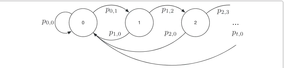
The CDE can be modeled following the infinite Markov chain in Figure 2. The stateE(n) = 0 means that in time n, the transmission exists. Similarly, the stateE(n) = t, fort =0, means that the samplen−twas the last to be transmitted. The transition matrix (with dimensionT → ∞) that describes the process of the CDE is
TCDE=
From the stationary condition in (21), we can obtain the following relations:
It is easy to observe that there are infinite solutions for the transition probabilitiespi,j. Thus, we address the design and the corresponding performance in the follow-ing sections.
4.4 Approximations for the downsampling distortion of the CDE-PD and CDE-SD
Figure 2Infinite Markov chain that models the encoder CDE.
to each statetof the MC. Therefore, we define the thresh-oldtas the threshold value applied to the statet.
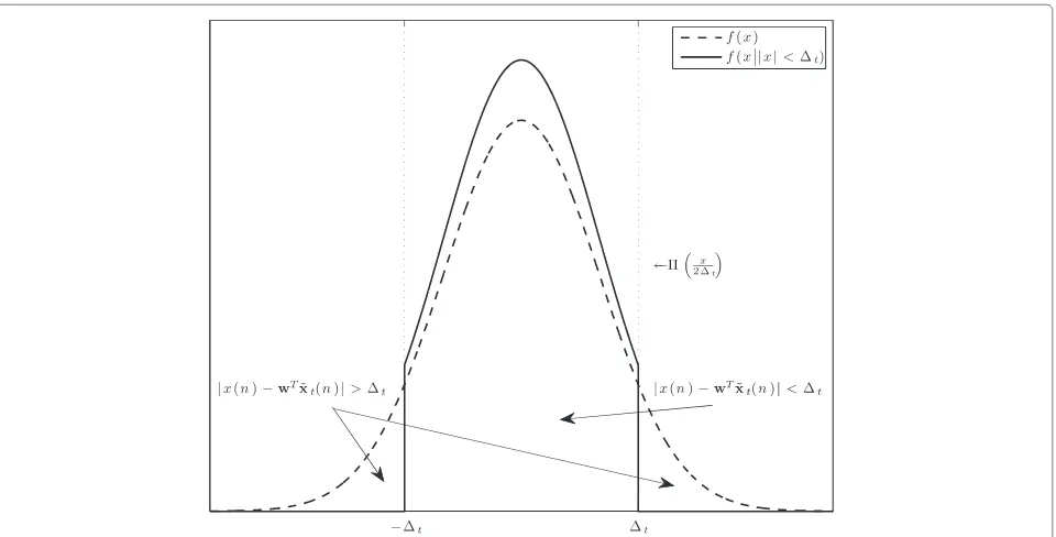
The condition in (7) modifies the probability density function (pdf ) of the error.
Definition 6.Let the conditional pdff(x|x|< t)be the
Moreover, therectangular function(x)is defined as fol-lows:(x) = 0 if|x| > 0.5,(x) = 1 if|x| < 0.5, and
Proof.Letxdefine the random variable
x∼ {x1|x|< t}, (28)
Applying the same relation as that in (30), we obtain
var(x)=β−1(t)
that comes from the relation
Definition 7.We define the conditional function h(σ2|t):R→Ras
h(σ2|t)=var(x|x|< t). (38)
4.4.1 The pair CDE-PD
Lemma 2.LetMSECDE-PDt be defined as the mean square error when the observation vector is x˜t(n). Then, the MSECDE-PDt is an approximation of MSECDE-PDt (i.e., the error introduced by the CDE-PD pair at the state t) and defined as
MSECDEt −PD=h1−ρ2+ρ2MSECDEt−1−PD|t
MSECDEt −PD. (39)
Proof. Fort =1, the error MSECDE-PD1 follows the condi-tional variancebsuch that
MSECDE-PD1 =E(x(n)−wTx˜1(n))2|x(n)−wTx˜1(n)|< 1
=E(ρx(n−1)+z(n)−ρx(n−1))2||ρx(n−1) + z(n)−ρx(n−1)|< 1]
=Ez(n)2||z(n)|< 1]
= ∞
−∞z(n)
2f(z(n)|z(n)|<
1)dz(n). (40)
Using Definition 7 and sincez(n) ∼ N0,σz2where
σ2
z =1−ρ2, the MSECDE1 −SDis
MSECDE-PD1 =h1−ρ2|1
. (41)
Fort = 2, the available knowledge is twofold: (1) we know that|x(n)−wTx˜
2(n)| < 2, and (2) we also know
that int=1 the error was|z(n−1)|< 1. Therefore, the MSECDE-PD2 can be written as
MSECDE-PD2 =E(x(n)−wTx˜2(n))2||x(n) (42) − wTx˜
2(n)|< 2,|z(n−1)|< 1
,
=E(ρx(n−1)+z(n)−ρwTx˜1(n−1))2||x(n)
− ρwTx˜
1(n−1)|< 2,|z(n−1)|< 1
,
=E(ρz(n−1)+z(n))2||ρz(n−1) + z(n)|< 2,|z(n−1)|< 1
.
The expectation in (42) can be computed as
MSECDE-PD2 = ∞
−∞(z(n)+ρz(n−1))
2f(z(n)+ρz(n−1)
|z(n−1)|< 1,|ρz(n−1)
+z(n)|< 2)dz(n)dz(n−1). (43)
This expression is actually the computation of the vari-ance of a bivariant truncated normal distribution. The solution of a singly truncated bivariate distribution can be found in [23]. For higher orders, i.e.,t > 2, the solu-tion refers to the calculasolu-tion of the variance of a truncated multivariate normal distribution [24]. Although a solution already exists in the literature, it turns out to be quite complex. Moreover, its complexity increases int. For that reason, we are considering the following approximation:
{ρz(n−1)+z(n)|z(n−1)|< 1}
∼ N0,E(ρz(n−1)+z(n))2|z(n−1)|< 1, (44)
Figure 3Qualitative representation of the conditional pdff(x|x|< t).Due to the measurements that|xs(n)−wTx˜t(n)|< tare not
introducing error since they are not estimated. The parametertshould be chosen in order to guarantee that a fractionγof the total
but in the general case, it does not necessar-ily follow a Gaussian distribution. The variance E(ρz(n−1)+z(n))2|z(n−1)|< 1 so, the MSE introduced att=2 is approximated by
MSECDE-PD2 h
1−ρ2+ρ2MSECDE-PD1 |2
. (46)
It is easy to conclude that for the general case t, the MSECDE-PDt is
MSECDE-PDt MSECDE-PDt =h1−ρ2+ρ2MSECDE-PDt−1 |t
.
(47)
Hence, theD(CDE,PD)is approximated by
D(CDE,PD) ∞
t=0
PtMSECDE-PDt . (48)
However, this is still an open problem. It is because the values ofPt are not determined yet. We study this issue afterwards in Section 4.5.
4.4.2 The pair CDE-SD
Ifxˆ(n)is constructed from a linear prediction using the LWF, the MSE in prediction is directly σz2 = 1 − ρ2. However, using other strategies, the error will increase as we have seen in (18). In particular, the pair CDE-SD con-structsxˆ(n) as the last transmitted sample, i.e., xˆ(n) = x(n−t). This prediction scheme introduces an error not only due toz(n)but also due tox(n).
Lemma 3.The MSECDEt −SD is an approximation of MSECDEt −SD(i.e., the error introduced by the CDE-SD pair at the state t) and it is defined as
MSECDEt −SD=h1−ρ2+MSECDEt−1−SD|t
≤MSECDEt −SD. (49)
Proof.Similarly to the CDE-SD, for t = 1 the error MSECDE1 −SDfollows the conditional variance such that
MSECDE1 −SD=E(x(n)−x(n−1))2|x(n)−x(n−1)|<1
Fort=2 the available information is twofold: (1) we know that|x(n)−x(n−2)| < 2, and (2) we also know that
To solve the MSECDEt −SDin a recursive way may be harder than for the CDE-PD case. It is because we cannot apply directly the conditional function since the expectation in (53) is not of the formh(σ2
x|) =E
x2|x|< . Hence, to simplify, we propose a lower bound for (53) such that
MSECDE2 −SD≥E(z(n−1)+z(n))2|z(n−1) +z(n)|< 2,|z(n−1)|< 1
. (54)
One can easily check that it is in fact a lower bound since
E(z(n)−(1−ρ)x(n−1))2≤E(ρz(n)−(1−ρ2)x(n−1))2
1−ρ2≤2(1−ρ). (55)
Our proposed lower bound is very close to the real value for high values ofρ. Using the same approximation as in the CDE-PD case, and after some simple algebra, we can find the lower bound of (53) as
MSECDE2 −SD=h
It is easy to conclude that for the general case t, the MSECDEt −SDis
Hence, theD(CDE,SD)is lower-bounded by
D(CDE, SD)≥ ∞
t=0
As for the case of the CDE-PD pair, this is still an open problem, and it is studied afterwards in Section 4.5.
4.5 Design of the CDE-SD and the CDE-PD
From the design point of view, our aim is to obtain a set of
t’s that assure a coding rate at the CDE ofγ. However, there are infinite solutions as we pointed out in (24). That is why we propose two possible approaches to face with the design oft:
• Fixedt, i.e.,t=for allt.
• Variabletin order to maintain constant transition probabilities, i.e.,pt−1,t=pfor allt.
4.5.1 Fixedtdesign
This is probably the simplest approach to design the CDE since the encoder does not have to change the value oft according to the current state sincet=for allt.
First, we want to make explicit the existing relation betweenandpt−1,t, as
pt−1,t()=
−ft(x)dx, (59)
whereft(x)is the pdf of the error at statet.
Following the assumption in (44), the variable x(n) − ˆ
x(n)follows a Gaussian distribution with zero mean and variance MSECDEt (), where
where erf(x) is the error function of x. Using the result in (24), we can numerically approximate that assures P0=γ as the unique solution of
The solution offor the different values ofγandρcan be graphically seen in Figure 4.
4.5.2 Variabletdesign
This approach allows for a slightly easier computation of the values oft. The main difference with the previous design scheme is that we can use the result in the following lemma:
Lemma 4.The uniform solutions of the non-zero transi-tion probabilities and for the statransi-tionary probability vector are to compute the probability of each state, and considering (23), we get
Pt=γpt=γ (1−γ )t. (65)
Hence,tis directly
t=
To graphically validate our design framework, we have proposed the following experiment:
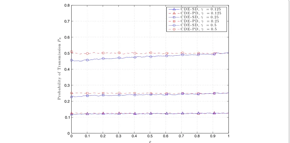
Experiment 1.We have simulated the CDE-SD and the CDE-PD for γ =[ 1/8 1/4 1/2] and for ρ ∈[ 0, 1]. The signal has been generated following the AR-1 process of 5, 000samples (for each value ofρ). We have computed the probability of transmission P0obtained using our threshold design framework.
From Experiment 1, we have plotted the probability of transmissionP0as a function ofρ and for each value of
Figure 4Numerical solution offor the fixedtdesign.The values ofγareγ= {0.125, 0.25, 0.5}, the values ofρareρ= {0.25, 0.5, 0.75}, and
the value ofTis 100. The red cross marks are thesolutions for a givenρandγ.
5 Downsampling distortion of other typical strategies
In order to measure the performance of the CDE, we also evaluate the performance of different encoder-decoder pairs in terms of the downsampling distortion. These are DDE-SD, DDE-PD, PDE-SD, and PDE-PD.
5.1 The pair DDE-SD
The index t denotes the time spacing between the last available sample with the current one. Thus, we can com-pute the MSEDDE-SDt using the result in (18) for each observation vectorx˜t. Therefore, the downsampling dis-tortion will be the sum of the MSE contributions for each
state. Applying the definition of stationary probability vector in Definition 5, we extract that Pi = Pj for all i,j= 0, 1,. . .,T. Since we impose a coding rate ofγ, the probability of transmission, i.e.,P0, isP0=1/T =γ. The stationary probability vector isp=γ1. Hence, the down-sampling distortion for the DDE-SD can be computed as
The knowledge of the correlation parameters is avail-able at the PD, and hence, it can predict the non-transmitted samples using the LWF. Following Theorem 1, the MSEDDE-PDt = 1 − ρ2t. Hence, the downsampling distortion for the DDE-PD can be computed as
D(DDE,PD)=
The PDE can also be modeled following the infinite MC in Figure 2. Hence, the transmission matrixTCDEhas the same structure thanTCDEin (22), and the expressions (23) and (24) are valid as well. However, the rest is different.
For simplicity, we assume that allpt−1,t are equal, i.e., theuniform probabilitycase. The results of Lemma 4 also apply here. It gives us two main advantages:
1. It is the easiest solution to be implemented in practice. The source decides either to transmit or not regardless of what the current statet is.
2. It reduces the problem to a closed-form solution.
Using the results for the MSEtin (18) corresponding to the decoder SD, we obtain
D(PDE,SD)=
The MSE associated to the statetobeys Theorem 1. The downsampling distortion for the PDE-PD can be com-puted as
In this section, we evaluate and compare the performance of the different encoder-decoder pairs as a function of the downsampling distortion. Moreover, we introduce an experimental evaluation in order to confirm the validity of our theoretical results. For that, we have generated a sig-nalx(n) as a sequence of 5, 000 samples using the AR-1 model in (2) and for different values of the autoregressive parameterρ ∈[ 0, 1] with resolution 0.01. The results are computed forγ =[ 1/8, 1/4, 1/2].
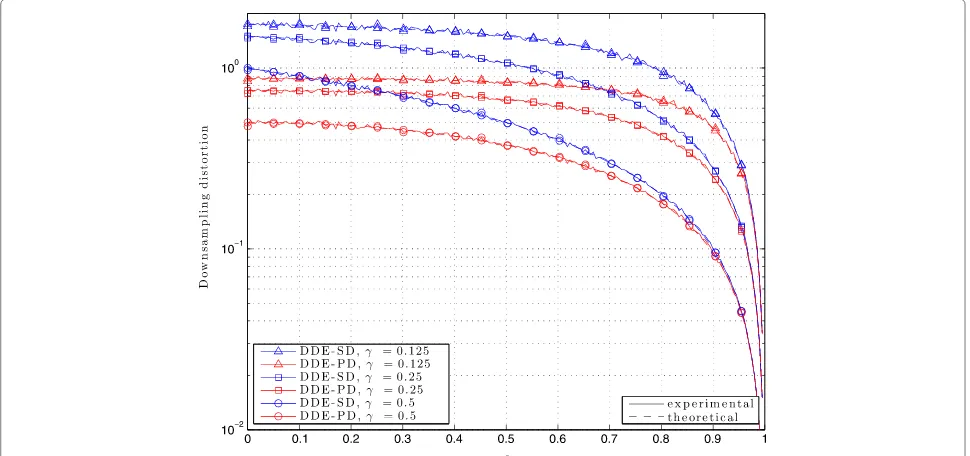
6.1 The pair DDE-SD and the pair DDE-PD
We analyze the downsampling distortion for the DDE-SD and DDE-PD pairs. We compare the theoretical results with the experimental results. So, Figure 6 confirms the validity of our theoretical model for the downsampling distortion.
Also, we compare the difference in performance accord-ing to the decoder used. The PD takes into account the signal correlation information in the decoding process, and hence, the total performance is increased notably for low values ofρ. On the contrary, ifρ→1, both decoders perform similarly sincex(n)−ρtx(n−t)≈x(n)−x(n−t). In Figure 6, we can also graphically evaluate the impact of γ. In our scenario, the signal x(n) is transmitted by the DDE in{8, 4, 2} times following a uniform pattern. It is easy to see that the larger the γ, the lower is the distortion. However, there exists a trade-off between the downsampling distortion and the compression rate.
6.2 The pair PDE-SD and the pair PDE-PD
are similar to the ones established in Section 6.1. For the sake of clarity, we compare the downsampling distortion results of the different pairs later in Section 6.4.
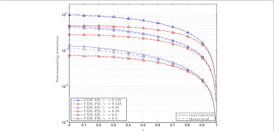
6.3 The pair CDE-SD and the pair CDE-PD
The performance of the previous encoder-decoder pairs can be notably improved by conditional transmission at the encoder site. In particular, we study and compare the downsampling distortion of the two design approaches, i.e., the fixedtdesign and the variabletdesign (with uniform transition probabilities), depicted in Figures 8 and 9, respectively. As in the previous pairs, we compare both the experimental results with the theoretical results. However, in that case, our theoretical results are limited to an approximation rather than the real system perfor-mance. Even so, we can observe that the approximations are very accurate for all the different simulations. For the case of CDE-PD, the approximation is so close to the sys-tem performance that the difference cannot be observed because it is masked by the small amount of noise due to the simulation. For the case of CDE-SD, the difference is slightly bigger because of the approximation in (55).
Another conclusion is that the downsampling distor-tion is notably higher for the fixed design. It is because their transition probabilities pt−1,t are increasing in t, and it facilitates to achieve higher states t in the MC with higher probability (i.e., higher MSEt’s). On the con-trary, the variable design concentrates the states in lower tvalues.
From a practical point of view, the CDE is simpler if it follows a fixed design since the encoder only needs to know the value of and also it does not need to track the current statet. However, from a computational point of view, the variable approach is simpler since it can be computed analytically, instead of numerically.
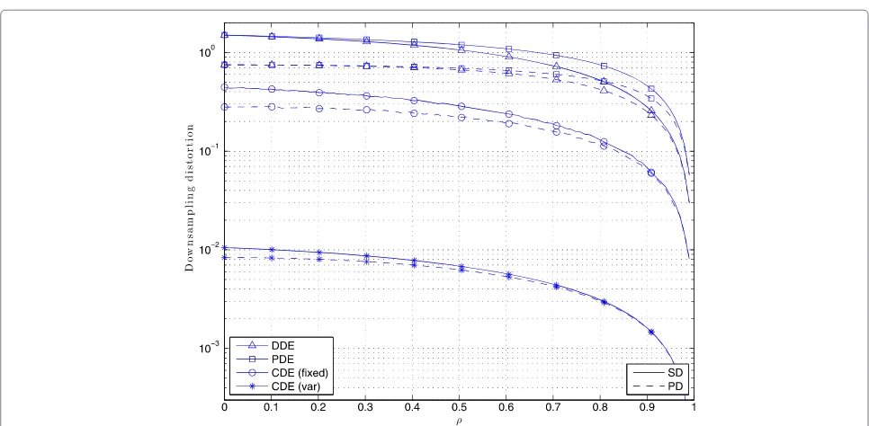
6.4 Comparison of the downsampling distortion
Finally, we compare the performance of the different encoder-decoder pairs. Although Figure 10 does not pro-vide any extra information, it allows us to better compare the performance of the different schemes. For the sake of simplicity, we only compare the theoretical results for the case ofγ =0.25.
It can be observed that the performance of the DDE and PDE are similar. However, the deterministic encoder works slightly better since it only uses the lowest γ−1 states of the finite MC while PDE uses higher states that are related to higher errors. However, the main disadvantage of the DDE in front of the PDE is its lack of flexibility since the uniform solution is only valid for natural values of γ−1. Furthermore, the PDE with uniform transition probabilities does not need to track the current state t of the process, and hence, it is simpler.
The big hop in performance is observed for the CDE. This encoder eliminates the transmissions of the samples with the most redundant information. Thus, only the most ‘unpredictable’ samples are transmitted.
Figure 6Experimental and theoretical downsampling distortion of the pairs DDE-SD and DDE-PD as a function ofρ.The coding rates are
Figure 7Experimental and theoretical downsampling distortion of the pairs PDE-SD and PDE-PD as a function ofρ.The coding rates are
γ= {0.125, 0.25, 0.5}. Different markers denote different values ofγ; curves in blue represent the SD, whereas curves in red represent the PD; solid lines represent experimental results, and dashed lines represent theoretical results.
7 Conclusions
In this chapter, we have evaluated the performance of dif-ferent encoding-decoding strategies in order to reduce the number of transmitted samples and hence to decrease the power spent in transmission. We have presented them as
an energy-efficient solution for the wireless sensor net-work communication problem. In particular, we define the downsampling distortion function in order to evaluate the performance in terms of the trade-off between com-pression rate and distortion at the fusion center of the
Figure 8Experimental and theoretical approximation of downsampling distortion of CDE-SD/CDE-PD pairs following a fixedtdesign.
Figure 9Experimental and theoretical approximation of downsampling distortion of CDE-SD/CDE-PD pairs following a variablet design.The coding rates areγ= {0.125, 0.25, 0.5}. Different markers denote different values ofγ; curves in blue represent the SD, whereas curves in red represent the PD; solid lines represent experimental results, and dashed lines represent theoretical results.
combination of three downsampling encoders, which are the DDE, the PDE, and the CDE, with two decoders: the SD and the PD.
We have obtained closed-form expressions for the pairs DDE-SD, DDE-PD, PDE-SD, and PDE-PD and accurate approximations for CDE-SD and CDE-PD. Moreover, we
have proposed two strategies in order to design the threshold of the condition in the CDE, i.e., the fixed threshold design and the variable threshold design.
The simulation results validate our theoretical results. Furthermore, we have compared the performance of the different pairs and showed the impact of taking into
Figure 10Comparison of the downsampling distortion of the different encoding-decoding pairs as a function ofρ.The coding rate is
account the signal model in the encoding-decoding pro-cess. Hence, the pair CDE-PD (with variable threshold design) outperforms by far the rest of the studied strate-gies. However, extending the CDE analysis for higher order AR models or even for other time-correlated signal models remains as an open problem.
Endnotes
a Notation. Boldface uppercase letters denote matrices,
boldface lowercase letters denote column vectors, and italics denote scalars.(·)T,(·)∗,(·)Hdenote transpose, complex conjugate, and conjugate transpose (Hermitian), respectively. [X]i,jand [x]iare the (ith,jth) element of matrixXand theith position of vectorx, respectively. [X]idenotes theith column ofX.| · |is the absolute value.arepresents the Euclidean norm ofa. Letaˆrefer to the estimated value of variablea.E[·] is the statistical expectation. Function erf(·) represents the error function.
b Theconditional varianceof a continuous random
variableXgiven the conditionY=yis defined as var(X|Y=y)=E[X2|Y=y]=#−∞∞ x2f(X|Y=y)dx, wheref(X|Y=y)is the conditional pdf ofXgivenY=y.
c It comes from the definition of the cumulative density
function of a Gaussian variable such that #a
The authors declare that they have no competing interests.
Acknowledgements
This work is supported by the Spanish Government under project TEC2011-28219 and the Catalan Government under grant 2009 SGR 298. Received: 14 January 2013 Accepted: 30 April 2013
Published: 10 May 2013
References
1. CK Toh, Maximum battery life routing to support ubiquitous mobile computing in wireless ad hoc networks. Commun. Mag., IEEE.39(6), 138–147 (2001)
2. O Younis, S Fahmy, HEED: a hybrid, energy-efficient, distributed clustering approach for ad hoc sensor networks. Mobile Comput. IEEE Trans.3(4), 366–379 (2004)
3. R Mudumbai, D Brown, U Madhow, H Poor, Distributed transmit beamforming: challenges and recent progress. Commun. Mag., IEEE.
47(2), 102–110 (2009)
4. K Zarifi, S Zaidi, S Affes, A Ghrayeb, A distributed amplify-and-forward beamforming technique in wireless sensor networks. Signal Process., IEEE Trans.59(8), 3657–3674 (2011)
5. S Pradhan, J Kusuma, K Ramchandran, Distributed compression in a dense microsensor network. Signal Process. Mag., IEEE.19(2), 51–60 (2002) 6. N Sun, J Wu, Optimum sampling in spatial-temporally correlated wireless
sensor networks. EURASIP J. Wireless Commun. Netw.2013, 5 (2013) 7. D Neuhoff, R Gilbert, Causal source codes. Inf. Theory, IEEE Trans.28(5),
701–713 (1982)
8. T Weissman, N Merhav, On causal source codes with side information. Inf. Theory, IEEE Trans.51(11), 4003–4013 (2005)
9. M Derpich, Improved upper bounds to the causal quadratic rate-distortion function for Gaussian stationary. Inf. Theory, IEEE Trans.
58(99), 3131–3152 (2012)
10. H Viswanathan, T Berger, Sequential coding of correlated sources. Inf. Theory, IEEE Trans.46, 236–246 (2000)
11. R Zamir, Y Kochman, U Erez, Achieving the Gaussian rate distortion function by prediction. Inf. Theory, IEEE Trans.54(7), 3354–3364 (2008) 12. JB O’Neal, Delta-modulation quantizing noise-analytic and computer
simulation results for Gaussian and television input signals. Bell Syst. Tech. J.45, 117–141 (1971)
13. EN Protonotarios, Slope overload noise in differential pulse code modulation systems. Bell Syst. Tech. J.46, 2119–2161 (1967)
14. TM Cover, JA Thomas,Elements on Information Theory. (Wiley, New York, 1991)
15. JB O’Neal, Signal-to-quantizating-noise ratio for differential PCM. IEEE Trans. Commun. Technol.19, 568–570 (1971)
16. N Farvardin, J Modestino, Rate-distortion performance of DPCM schemes for autoregressive sources. Inf. Theory, IEEE Trans.31(3), 402 –418 (1985) 17. O Guleryuz, M Orchard, On the DPCM compression of Gaussian
autoregressive sequences. Inf. Theory, IEEE Trans.47(3), 945–956 (2001) 18. R Rugin, A Conti, G Mazzini, inProceedings of the 15th International
Conference on Software, Telecommunications and Computer Networks, 2007. SoftCOM 2007. Experimental investigation of the energy
consumption for wireless sensor network with centralized data collection scheme (Split-Dubrovnik, 27–29 Sept 2007), pp. 1–5
19. Q Wang, Traffic analysis, modeling and their applications in
energy-constrained wireless sensor networks: on network optimization and anomaly detection. (Mid Sweden University, 2010) . http://urn.kb.se/ resolve?urn=urn:nbn:se:miun:diva-10690. Accessed 15 July 2012 20. T Hashimoto, S Arimoto, On the rate-distortion function for the
nonstationary Gaussian autoregressive process. Inf. Theory, IEEE Trans.
26(4), 478–480 (1980)
21. S Haykin,Adaptive Filter Theory, 4th edn. (Prentice Hall, Upper Saddle River, 2001)
22. J Barcelo-Llado, A Morell, G Seco-Granados, Enhanced correlation estimators for distributed source coding in large wireless sensor networks. IEEE Sensors J.12(9), 2799–2806 (2012)
23. S Rosenbaum, Moments of a truncated bivariate normal distribution. J. R. Stat. Soc. Ser B (Methodological).23(2), 405–408 (1961)
24. BG Manjunath, Wilhelm S,Moments calculation for the double truncated multivariate normal density (Social Science Research Network 2009). http:// dx.doi.org/10.2139/ssrn.1472153. Accessed 20 Aug 2012
doi:10.1186/1687-6180-2013-101
Cite this article as:Barceló-Lladó et al.:Conditional downsampling for energy-efficient communications in wireless sensor networks. EURASIP Journal on Advances in Signal Processing20132013:101.
Submit your manuscript to a
journal and benefi t from:
7Convenient online submission
7Rigorous peer review
7Immediate publication on acceptance
7Open access: articles freely available online
7High visibility within the fi eld
7Retaining the copyright to your article