Prediction of the geomagnetic storm associated
D
st
index
using an artificial neural network algorithm
Samuel Kugblenu, Satoshi Taguchi, and Takashi Okuzawa
Department of Electronic Engineering, University of Electro-Communications, Tokyo 182-8585, Japan
(Received July 5, 1997; Revised March 19, 1999; Accepted March 20, 1999)
In order to enhance the reproduction of the recovery phase Dst index of a geomagnetic storm which has been shown by previous studies to be poorly reproduced when compared with the initial and main phases, an artificial neural network with one hidden layer and error back-propagation learning has been developed. Three hourly Dst values before the minimumDstin the main phase in addition to solar wind data of IMF southward-componentBs, the total strength Btand the square root of the dynamic pressure,
√
nV2, for the minimumD
st, i.e., information on the main phase was used to train the network. Twenty carefully selected storms from 1972–1982 were used for the training, and the performance of the trained network was then tested with three storms of different Dst strengths outside the training data set. Extremely good agreement between the measuredDstand the modeled Dsthas been obtained for the recovery phase. The correlation coefficient between the predicted and observed Dstis more than 0.95. The average relative variance is 0.1 or less, which means that more than 90% of the observedDstvariance is predictable in our model. Our neural network model suggests that the minimumDstof a storm is significant in the storm recovery process.
1.
Introduction
The development of a magnetic storm is best identified at low latitudes by large decreases in theH component of the Earth’s magnetic field, and consequently in the Dst index, a quantity derived and introduced by Sugiura (1964) as a measure of the magnetic disturbance level on the Earth.
Geomagnetic storms, illustrated by Dst, typically have three phases: initial, main, and recovery phases. The initial phase is caused by an increased solar wind dynamic pres-sure acting on the magnetosphere. The increased prespres-sure compresses the dayside magnetosphere, forcing the magne-topause current closer to the Earth, and at the same time increasing it. The magnitude of the initial phase has been shown to be proportional to the square root of the solar wind dynamic pressure,√nV2(Ogilvieet al., 1968; Siscoeet al.,
1968), wheren is the solar wind density and V, the solar wind speed.
The main phase is due to an increase in energetic ions and electrons in the inner magnetosphere, where they be-come trapped on closed magnetic field lines and drift around the Earth, thus creating the ring current. The storm-time ring current has been shown to consist of solar wind ions and ionospheric-origin ions. H+ ions carry the major frac-tion of energy in the ring current almost throughout the storm, but O+ions prevail near the maximum of the main phase, particularly for large storms (Gloeckler and Hamilton, 1987; Hamiltonet al., 1988). Recent studies (Daglis, 1997; Hamilton, 1997) have confirmed the significant contribution of O+ions to the minimumDstvalue; that is, the minimum
Copy right cThe Society of Geomagnetism and Earth, Planetary and Space Sciences (SGEPSS); The Seismological Society of Japan; The Volcanological Society of Japan; The Geodetic Society of Japan; The Japanese Society for Planetary Sciences.
Dstshows a remarkable correlation with fractional O+ con-centration which can attain values as large as 70% for storms withDst≤ −300 nT. The main phase was also found to be associated with sustained southward IMF-Bz(Rostoker and F¨althammar, 1967).
Charge exchange and Coulomb scattering have both been identified as major loss processes responsible for the decay of the ring current during the recovery phase of storms (Smith and Bewtra, 1978; Foket al., 1991). Typical H+ and O+ lifetimes for each of these two processes are comparable to days, characteristic of the slow recovery inDstfollowing the main phase of a storm. However, since the charge-exchange lifetime of O+is considerably shorter than the H+lifetime for ring current energies (≥40 keV), Smith and Bewtra (1978) have suggested that increased O+influences the decay rate of the ring current.
Many different methods (Baker, 1986) have been used for predicting geomagnetic storms, such as ordinary statistical methods (which include visual correlation analyses as well), linear filtering and artificial intelligence methods. Most of these relationships are based on parameter studies in a cause-and-effect manner. Solar wind parameters constitute the causal variables, while geomagnetic indices (Dst, AE,AL, or AU) are the designated effect variables.
Burtonet al.(1975) proposed an empirical linear relation-ship for predicting theDstindex from the knowledge of the solar wind velocity, density, and the southward component of IMF. In particular, Burtonet al.developed an equation for the rate of change of pressure correctedDst, showing that it was a balance between injection and decay out of the ring current. They found that decay rate for the recovery phase depends on the present strength of the ring current (Dst).
The method of linear filtering prediction was used by
Iyemoriet al.(1979) to predict geomagnetic-storm indices. This technique allows one to empirically determine the most general linear relationship between a solar wind input func-tion and a geomagnetic disturbance output funcfunc-tion, tak-ing time delays and frequency response into consideration (Clauer, 1986). Iyemoriet al.(1979), and Iyemori and Maeda (1980) used IMF-Bzas an input function, and their output
function was one of the geomagnetic indices,Dst,AE,AL, andAU. They concluded that using a single input solar-wind function is not enough to predict completely a geomagnetic disturbance based on the assumption of a linear system. They attributed this inability to a possible nonlinear response of the magnetosphere.
Artificial neural network (ANN) models enjoyed a resur-gence in popularity as a prediction tool during the late 1980s, as a consequence of the discovery of the backpropagation of errors learning algorithm. One of the most unique property of these ANNs is their ability to generalize to new situa-tions after having been trained on a number of examples of a relationship. They can then induce a complete relation-ship that interpolates and extrapolates from the examples. ANNs therefore offer the possibility to study large complex nonlinear systems of highly inter-correlated data.
Several ANN models (e.g., Freeman et al., 1993; Lundstedt and Wintoft, 1994; Gleisner et al., 1996) have shown good performance for the reproduction of Dst. Al-though the reproduction of the initial and main phases was excellent, there was somewhat difficulty in reproducing the recovery phase well. In this study, in order to enhance the recovery phase reproduction, we use a feed forward multi-layer neural network with error-backpropagation learning al-gorithm. This network is trained using three hourly values before the minimum Dst in the main phase designated as
Dst(−1), Dst(−2), and Dst(−3), in addition to solar wind parameters for the minimum Dst, i.e., the magnetic field strengthBt, the southward IMF componentBsand the solar
wind dynamic pressure√nV2. In other words, we used
in-formation only on the main phase for the network training. This trained network is able to reproduce the recovery phase with high accuracy.
2.
Arti
fi
cial Neural Networks
ANNs make up a new approach to the computation that involves developing mathematical structures with learning ability. This approach is the result of academic investiga-tions to model the human nervous system learning. ANN is essentially a group of interconnected computing elements (i.e., neurons).
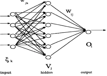
The multi-layer feed-forward error backpropagation algo-rithm (Hertzet al., 1991, for detail) was used in this study. This network belongs to the class of supervised networks, i.e., it learns from known answers. Typically, the network is arranged in layers of neurons (nodes), where every neuron in a layer computes the sum of its inputs and passes this sum through a nonlinear function (an activation function) as its output. Each neuron has only one output, but this output is multiplied by a weighting factor if it is to be used as an input to another neuron (in a next higher layer). There are no connections among neurons in the same layer.
Figure 1 shows a typical three layer network structure. The
Fig. 1. A three-layered neural network.
input, hidden, and output layers are denoted byk, j, andi, respectively. For a given pattern,μ, a neuron jin the hidden layer receives, from a neuronkin the input layer, a net input signal given by
xμj =
k
wj kξkμ+bk (1)
whereξkμis the input signal fed to neuronkin the input layer, andwj kis the connection strength between neuron jin the hidden layer and neuronkin the input layer, whilebkis a bias connected to the input layer. The bias is an additional input to a neuron that serves to normalize its output, and normally has a constant activation of 1.
The outputVj produced by the jth neuron in the hidden layer is related to the activation value for that neuron, by a transfer functiongh(x)which will be defined later, in such a
way as
Vjμ=gh(xμj)=gh
k
wj kξkμ+bk
. (2)
A neuroni in the output layer receives this signal from the neuron jin the hidden layer as input, and similarly produces an output,Oiμ, which is related to the activation value for that neuron, by a transfer functiongo(x)(which will be assumed
to be the same form ofgh(x)in this paper)
Oiμ=go(xiμ)=go
j
Wi jVjμ+bj
. (3)
The biases in the equations, bk and bj, can be omitted as they can be considered as an extra input of unit value connected to all units in the network. Thefinal net output for an input patternμ,(μ=1, . . . ,p)can be then described by
Oiμ=go
Wi jgh
wj kξkμ
. (4)
linear functions is again a linear function. It is the nonlin-earity (i.e., the capability to represent nonlinear functions) that makes multi-layer networks so powerful. Almost any nonlinear function is applicable. For backpropagation learn-ing, however, it must be differentiable and saturating at both extremes. Sigmoid functions such as the logistic and hyper-bolic tangent functions, and the Gaussian function are the most common choices. If the transfer functions were chosen to be linear, then the network would become identical to a linearfilter (Iyemori et al., 1979). A backpropagation net with nonlinear transfer functions could be thus regarded as a nonlinear generalization of a linearfilter (see Gleisner and Lundstedt, 1997).
The steepness of the logistic sigmoid can be modified by a slope parameterσ. The more general sigmoid function (with range between 0 and 1) is given by
g(x)=gh(x)=go(x)=
1
1+exp(−σx) (5)
with its derivative as
g(x)=σg(x)[1−g(x)]. (6)
The slope may be determined such that the sigmoid function achieves a particular desired value for a given value ofx, the input (Fausett, 1994). In the present studyσhas been set to 4 for nonlinear multiregression analysis (Ichikawa, 1993).
The training of a network by backpropagation involves three stages: the feedforward of the input training pattern, the calculation and backpropagation of the associated error, and the adjustment of the weights. After training, application of the net involves only the computations of the feedforward phase. In order to train the network, input is shown to the net together with the corresponding known output, and if there exists a relation between the input,ξkμ, and the output, Oiμ, the netlearnsby adjusting the weights until an optimum set of weights that minimizes the network error is found and the network then converges.
The network error,E, which is defined as the sum of the individual errors over a number of examples, is given by
E =1
Substituting (4) for the net output,Oiμ, we have
E= 1 At the completion of a pass through the entire data set, all the nodes change their weights based on the accumulated derivatives of the error with respect to each weight. These weight changes move the weights in such a direction that the error declines most quickly. The standard learning al-gorithm which updates the weights can be expressed by the gradient descent rule, which means that each weight, say, wpq, changes by an amountwpqwhich is proportional to the gradient of the errorEat the present location.
For the hidden-to-output connections, the gradient descent rule gives the change in weight as
Wi jnew=W
and η stands for the learning rate. Similarly, the weight change for the input-to-hidden connections, is given by
wnew
The neural network software used for this work was orig-inally developed by Ichikawa (1993). The network structure is flexible to configure since all parameters are commuta-tive. Our model is a feed forward multi-layer network with error-backpropagation learning, and applied as a nonlinear, multi-variable least squares algorithm.
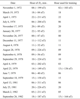
For both network training and prediction, we used the OMNI data set from the database of the National Space Science Data Center of NASA and the WDC-2 Data Cen-ter of Kyoto University. These data sets consist of hourly averages of the solar wind plasma and IMF data from var-ious spacecraft. Hourly average of Dst is also available in these databases. For the storm selection, we required that the storm be preceded by a relatively quiet period ofDst ac-tivity. Storms with large and sustained southward IMF were given priority in the selection process, as well as sudden in-creases in the velocity of solar wind, mostly above 450 km/s. Selection of storm events was, however, limited owing to in-completeness of solar wind data. Twenty storms of different intensities withDst≤ −30 nT were selected from the years of 1972, 1973, 1974, 1975, 1977, 1978, 1979, 1981, and 1982. These are shown in Table 1.
Table 1 also shows the hour and values of the minimum
Dst (peak value) for the 20 storms (column 2). When the solar wind data set corresponding to the minimum value of
Dst is not available in the database, the nearest hour having a complete data set was taken. This hour is indicated in column 3, where the hour is different from that of column 2 for November 1, 1972, April 25, 1979, and September 26, 1982 storm events.
The minimum Dstpeak value has been used in ring cur-rent energization studies. Pudovkin et al. (1985) used the hourly Dst peak value to study the relationship of the ring current energy to solar wind functions and to calculate the characteristics decay time. For our network training, there-fore, we made a data set consisting of minimumDstvalue in the main phase for each storm, which we designate Dst(0), the corresponding solar wind data (IMF total stengthBt, IMF
southward componentBs, and dynamic pressure
√
nV2) for
that hour, and 3 consecutive preceding hourly Dstvalues in the main phase. TheseDstvalues are designated byDst(−1),
Table 1. List of storms used for network training.
Date Hour ofDstmin. Hour used for training
November 1, 1972 08 (−199 nT) 02 (−103 nT)
March 19, 1973 18 (−84 nT) 18
April 1, 1973 22 (−211 nT) 22
July 6, 1974 06 (−204 nT) 06
November 17, 1975 20 (−89 nT) 20
January 30, 1977 22 (−95 nT) 22
November 26, 1977 00 (−87 nT) 00
December 11, 1977 11 (−112 nT) 11
August 4, 1978 11 (−32 nT) 11
August 28, 1978 09 (−226 nT) 09
September 6, 1978 09 (−56 nT) 09
September 29, 1978 10 (−224 nT) 10
April 4, 1979 03 (−202 nT) 03
April 25, 1979 14 (−149 nT) 13 (−136 nT)
June 7, 1979 06 (−40 nT) 06
September 18, 1979 15 (−158 nT) 15
April 13, 1981 06 (−311 nT) 06
July 25, 1981 20 (−226 nT) 20
March 2, 1982 05 (−211 nT) 05
September 26, 1982 18 (−187 nT) 15 (−164 nT)
as the known output parameter. A data set for one storm thus consists of a six parameter input and a corresponding one pa-rameter output. This is presented to the net during training. For prediction, we used the six parameters with no corre-sponding output parameter. This includes three preceeding previousDstvalues and the solar wind data set for each hour of a storm event.
Determination of the number of hidden nodes is a difficult task. Although some techniques have been used by different authors (e.g., Lundstedt and Wintoft, 1994), no established methods exist. We have therefore applied different network architectures with various number of hidden nodes and learn-ing rates to the network durlearn-ing trainlearn-ing in order to determine the best such parameters. A compromise for the bestfit has been found to be 7 nodes for the hidden layer and 0.15 for the learning rateη. This learning rate is the best among an applicable range of 0.05 to 0.2.
4.
Network Prediction
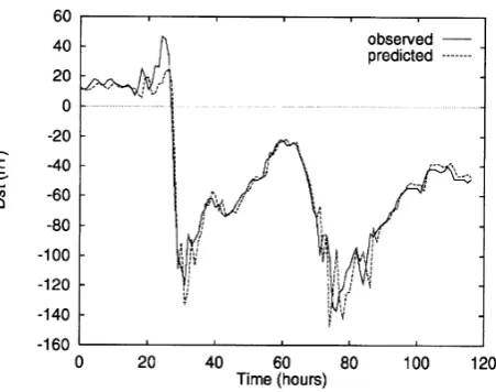
4.1 December 19, 1980 storm event
Our purpose is to reproduce the Dstindex for the recov-ery phase using data from the main phase, nevertheless we apply our trained ANN to the period starting with several hours before the beginning of the initial phase. A sudden in-crease in theDstplot at 29th hour (05:00 UT, December 19) defines the beginning of the initial phase of the storm. The
initial phase lasted for roughly about 10 hours. This was fol-lowed by a very rapid decrease inDstreaching its minimum approximately in the 42nd hour (18:00 UT, December 19). This constitutes the main phase. The Dst index then began a rapid recovery atfirst, followed by a long and slow one until the 119th hour. TheDstminimum marks the beginning of the recovery phase during which the ring current decays. This event has 119 data points.
Figure 2 shows the prediction result for the storm of De-cember 19, 1980 compared with observed Dst. The solid and broken lines represent the observation and prediction, respectively. Good agreement between the measured Dst and the predicted one exists in the recovery phase.
The recovery phase, which is more dependent on the in-ternal processes of the magnetosphere, is bound to be repre-sented by theDsthistory. The minimumDstshould also be well reproduced since main phase data were used in training the network. The initial phase appears to be well reproduced, but this is not the general trend as is shown later by the poor fitting of the initial phase in Fig. 5. However, it is interesting to reproduce somewhat theDstjump at the beginning of the initial phase. Considering that there is often a gradual de-crease in the dynamic pressure during the main phase where
in-Fig. 2. Observed and predicted Dst plot of December 19, 1980 storm.
The horizontal axis represents time from the beginning of December 18, 1980.
Fig. 3. Correlation plot of predictedDstand observedDstof December
19, 1980 storm.
crease in the dynamic pressure for the initial phase. Figure 3 shows correlation between the network prediction output and the target for the recovery phase, i.e., a period of time from the 18th hour of December 19 to the 23th hour of December 22. The correlation coefficient for this interval is 0.98. We also calculated the average relative variance (ARV), i.e., the mean squares error normalized by the variance of the data,
ARV = N
t=1(D(t)−O(t)) 2
N
t=1(D(t)− D)2
(13)
and the root mean squares error (RMSE):
RMSE=
1
N
N
t=1
(D(t)−O(t))2 1/2
(14)
for the same interval, whereD(t),DandO(t)denote ob-served, its averaged, and predictedDst, respectively. ARVis 0.04, which means that 96 percent of the observedDst vari-ance is predictable from both solar wind andDsthistory. The value ofRMSEis 11 nT, which is very small compared with the lowest peak value ofDst. This storm event has been also
Fig. 4. Observed and predictedDstplot of April 25–26, 1989 storm. The
horizontal axis represents time from the 3rd hour of April 25, 1989.
Fig. 5. Observed and predictedDstplot of May 8–12, 1981 storm. The
horizontal axis represents time from the biginning of May 8, 1981.
studied by Lundstedt and Wintoft (1994) for Dst network prediction. Our model shows much better performance in the recovery phase.
4.2 April 25–26, 1989 storm event
April 25–26, 1989 storm event (Fig. 4) began at the 7th hour of the 25th day of April, 1989. From a value of+13 nT,
Dst decreased sharply to a low value of−118 nT to com-prise the first stage of a two-stage main phase (Kamide et al., 1998). TheDst index then increased briefly to a value of−94 nT (due to a rise in IMF-Bzat that hour) beforefi
-nally falling to the minimum value of−132 nT. The Dst index began a disturbed, long-lasting and slow recovery un-til the 85th hour, which we defined as the end of the recovery phase. In this case, we selected 93 data points, and obtained good agreement between measured and predictedDst. The correlation coefficient between the measured and predicted
90 percent of the observedDstvariance is predictable. The value ofRMSEis 5.5 nT.
4.3 May 8–12, 1981 storm event
As shown in Fig. 5, this storm event has two distinct min-ima. The main phase started around the 25th hour of the event, and fell rapidly to thefirst minimum of−120 nT. The recovery phase started with the northward turning of the IMF until about the 62th hour, when the IMF turned southward again to produce another main phase. This was again fol-lowed by another northward turning of the IMF to produce the consequent recovery phase.
We used 117 data points to reproduce this storm. Figure 5 illustrates our result. The coefficient of correlation has been calculated to be 0.96. TheRMSE becomes 11 nT and the
ARVhas been found to be 0.07; that is, 93% of the storm is predictable.
5.
Discussion
Recently, Gleisneret al.(1996) have shown that the solar wind history for 18–24 hours, which is a longer time window than our 3 hours, is needed as input to a trained network in order to reproduce all phases of a geomagnetic storm. They developed a time-delay feed forward neural network based on a temporal sequence of solar wind data. Their networks showed better performance with larger temporal size of the input data sequence, and were able to reproduce 85% of the
Dst variance, which is quite an improvement on the earlier work of Lundstedt and Wintoft (1994). In our model 90% of
Dsthave been reproduced, at least, for the recovery phase of the three storm events.
The use of previousDstvalues as input has been suggested by Lundstedt and Wintoft (1994) as another way to model all phases of the magnetic storm. However, as the measuredDst is not instantaneously available, they proposed the use of the predictedDsta few hours back in time as input to the net. It is noted that Freemanet al.(1993) had already used previous
Dst data together with solar wind inputs to predict 1-hour ahead Dst for input to their Magnetospheric Specification and Forecast Model (MSFM). For input to their network, they used the hourly averages of the IMF-B, Bz, the solar
wind pressure, and Dst values for the four previous hours. Their output is the 1-hour aheadDstvalue.
Our model is consistent with the linear autoregressive moving average (ARMA)filter assumption that geomagnetic activityO, can be described as a function of a time series of both solar activityI, and the previous geomagnetic activity,
Ot =F(It−1,It−2, . . . ,It−TI,Ot−1,Ot−2, . . . ,Ot−TS) (15) whereTIis the system memory for solar wind inputs, andTS
is the memory for previous magnetospheric states. Nonlinear generalizations of thisfilter have been referred to as state-input space models (Vassiliadis et al., 1995). The linear autoregressive moving average (ARMA)filter is extensively discussed by Detman and Vassiliadis (1997). A direct ANN equivalent is the Elman recurrent network.
Wu and Lundstedt (1996), attempting to reproduce the recovery phase which was difficult to model with the net-works of Lundstedt and Wintoft (1994), used Elman recur-rent networks. The Elman network is an extension of the
multi-layer backpropagation networks with an addition of a feedback connection from hidden to input layers which al-lows the network to both detect and generate time-varying patterns. Their Elman network model obtained a relatively high correlation coefficient, i.e., 0.91, for a very long period of Dst (900 hours). For each storm period, however, their model does not always give a good fit to the observations. Our model uses three hours of observed Dsthistory, whilst their model depends on the feedback element to generate the decay rate; our network is updated with previously measured data, and in their case, it is updated with previously predicted data.
Vassiliadiset al.(1996) presented a method that converts an ARMA model to a physical model, namely, a nonlinear damped oscillator. This is expressed as a second order dif-ferential equation in terms of the Dstindex as
d2D
where the model parametersν,andαare determined lo-cally for many different levels of activity ofDstandEy, the input of solar-wind electric field. Our model can be con-sidered as a neural net generalization of such category of second-order differential equation.
The number of previous hourlyDstvalues included beside the solar wind data as input to the network may be signifi -cant in the modeling of the current Dst. Training sequences with one and twoDstvalues did not produce goodfits to the observed data (not shown here). The use of one Dst value as input produces overfitting (more positive) in the recovery phase, while the inclusion of two Dst values produces un-derfitting. The length ofDsthistory may be an indication of the timescale of the dissipation processes that determine the magnetospheric system memory.
We have used IMF-Btas input to our net, and investigated
its effect on the network output. We found that deficiency of the Btparameter in the input leads to poor modeling of the
initial stage of the recovery phase, implying that this stage is associated with IMF-Bt. Prediction is therefore improved
withBtas input.
6.
Conclusion
To reproduce the recovery phaseDstindex we have devel-oped a model by training the ANN with the Dst minimum, three hourly Dst values before the minimum in the main phase, and the solar wind data for the Dst minimum. This model has greatly enhanced the recovery phase reproduc-tion. This suggests that a process producing minimum Dst of a storm is significant in the storm recovery process. This may be related to the suggestion that the increased O+which dominates the ring current during storm maximum influences the decay rate of the ring current (Smith and Bewtra, 1978). Further work would be needed for the decisive reason for the significance of theDstminimum for the storm recovery process.
The data supply from World Data Center C2 of Kyoto University and NSSDC/NASA are gratefully acknowledged.
References
Baker, D. N., Statistical analyses in the study of solar wind-magnetosphere coupling, inSolar Wind-Magnetosphere Coupling, edited by Y. Kamide and J. A. Slavin, pp. 17–38, Terra Scientific Pub., Tokyo, 1986. Burton, R. K., R. L. McPherron, and C. T. Russell, An empirical relationship
between interplanetary conditions andDst,J. Geophys. Res.,80, 4204–
4214, 1975.
Clauer, C. R., The technique of linear predictionfilters applied to studies of solar wind-magnetosphere coupling, inSolar Wind-Magnetosphere Cou-pling, edited by Y. Kamide and J. A. Slavin, pp. 39–57, Terra Scientific Pub., Tokyo, 1986.
Daglis, I. A., The role of magnetosphere-ionosphere coupling in magnetic storm dynamics, inMagnetic Storms, edited by B. T. Tsurutani, W. D. Gonzalez, Y. Kamide, and J. K. Arballo, pp. 107–116, AGU, Washington, D.C., 1997.
Detman, T. R. and D. Vassiliadis, Review of techniques for magnetic storm forecasting, inMagnetic Storms, edited by B. T. Tsurutani, W. D. Gonza-lez, Y. Kamide, and J. K. Arballo, pp. 253–266, AGU, Washington, D.C., 1997.
Fausett, L.,Fundamentals of Neural Networks: Architectures, Algorithms, and Applications, 461 pp.,Prentice Hall, Englewood Cliffs, NJ 07632, 1994.
Fok, M.-C., J. U. Kozyra, A. F. Nagy, and T. E. Cravens, Lifetime of ring cur-rent particles due to Coulomb collisions in the plasmasphere,J. Geophys. Res.,96, 7861–7867, 1991.
Freeman, J., A. Nagai, P. Reiff, W. Denig, S. Gussenhoven, M. A. Shea, M. Heinemann, F. Rich, and M. Hairston, The use of neural networks to predict magnetospheric parameters for input to a magnetospheric forecast model, inProceedings of the International Workshop on Artificial Intel-ligence Applications in Solar Terrestrial Physics, edited by J. Joselyn, H. Lundstedt, and J. Trolinger, pp. 167–182, Lund, Sweden, 1993. Gleisner, H. and H. Lundstedt, Response of the auroral electrojets to the
solar wind modeled with neural networks,J. Geophys. Res.,102, 14269– 14278, 1997.
Gleisner, H., H. Lundstedt, and P. Wintoft, Predicting geomagnetic storms from solar wind data using time-delay neural networks,Ann. Geophys.,
14, 679–686, 1996.
Gloeckler, G. and D. C. Hamilton, AMPTEE ion composition results,Phys. Scr., T18, 73–84, 1987.
Hamilton, D. C., 5. Storm dynamics/ring current, inMagnetic Storms, edited by B. T. Tsurutani, W. D. Gonzalez, Y. Kamide, and J. K. Arballo, pp. 6–7, AGU, Washington, D.C., 1997.
Hamilton, D. C., G. Gloeckler, F. M. Ipavich, W. Studemann, B. Wilken, and G. Kremser, Ring current development during during the great geo-magnetic storm of February 1986,J. Geophys. Res.,93, 14343–14355,
1988.
Hertz, J., A. Krogh, and R. G. Palmer,Introduction to the Theory of Neu-ral Computation, lecture notes vol. 1, Santa Fe Institute Studies in the sciences of complexity, 327 pp., Addison-Wesley, Redwood City, CA 94065, 1991.
Ichikawa, H.,Layered Neural Networks, 184 pp., Kyoritu Pub., Tokyo, 108, 1993.
Iyemori, T. and H. Maeda, Prediction of geomagnetic activities from solar wind parameters based on the linear prediction theory, inSolar-Terrestrial Predictions Proceedings, Vol. 4, U.S. Dept. of Commerce, Boulder, CO, A-1–A-7, 1980.
Iyemori, T., H. Maeda, and T. Kamei, Impulse response of geomagnetic indices to interplanetary magneticfields,J. Geomag. Geoelectr.,31, 1–9, 1979.
Kamide, Y., N. Yokoyama, W. Gonzalez, B. T. Tsurutani, I. A. Daglis, A. Brekke, and S. Masuda, Two step development of geomagnetic storms,
J. Geophys. Res.,103, 6917–6921, 1998.
Lundstedt, H. and P. Wintoft, Prediction of geomagnetic storms from solar-wind data with the use of a neural network,Ann. Geophys.,12, 19–24, 1994.
Ogilvie, K. W., L. F. Burlaga, and T. D. Wilkerson, Plasma observations on Explorer 34,J. Geophys. Res.,73, 6809–6824, 1968.
Pudovkin, M. I., S. A. Zaitseva, and L. Z. Sizova, Growth and decay of magnetospheric ring current,Planet. Space Sci.,33, 1097–1102, 1985. Rostoker, G. and C.-G. F¨althammar, Relationships between changes in the
interplanetary magneticfield and the variations in the magneticfield at the earth’s surface,J. Geophys. Res.,72, 5853–5863, 1967.
Siscoe, G. L., V. Formisano, and A. J. Lazarus, Relation between geomag-netic sudden impulses and solar wind pressure changes—an experimental investigation,J. Geophys. Res.,73, 4869–4874, 1968.
Smith, P. H. and N. K. Bewtra, Charge exchange lifetimes for ring current ions,Space Sci. Rev.,22, 301–318, 1978.
Sugiura, M., Hourly values of equatorialDstfor the IGY,Ann. Int. Geophys. Year,35, 49, 1964.
Vassiliadis, D., A. J. Klimas, D. N. Baker, and D. A. Roberts, A description of solar wind magnetosphere coupling based on nonlinearfilters,J. Geophys. Res.,100, 3495–3512, 1995.
Vassiliadis, D., A. J. Klimas, and D. N. Baker, Nonlinear ARMA models for theDstindex and their physical interpretation, paper presented at the
Third International Conference on Substorms (ICS-3), Versailles, France, May 12–17, 1996.
Wu, J.-G. and H. Lundstedt, Prediction of geomagnetic storms from solar wind data using Elman recurrent neural networks,Geophys. Res. Lett.,
23, 319–322, 1996.