R E S E A R C H
Open Access
A RSSI-based parameter tracking strategy
for constrained position localization
Jinze Du
1,2*, Jean-François Diouris
2and Yide Wang
2Abstract
In this paper, a received signal strength indicator (RSSI)-based parameter tracking strategy for constrained position localization is proposed. To estimate channel model parameters, least mean squares method (LMS) is associated with the trilateration method. In the context of applications where the positions are constrained on a grid, a novel tracking strategy is proposed to determine the real position and obtain the actual parameters in the monitored region. Based on practical data acquired from a real localization system, an experimental channel model is constructed to provide RSSI values and verify the proposed tracking strategy. Quantitative criteria are given to guarantee the efficiency of the proposed tracking strategy by providing a trade-off between the grid resolution and parameter variation. The simulation results show a good behavior of the proposed tracking strategy in the presence of space-time variation of the propagation channel. Compared with the existing RSSI-based algorithms, the proposed tracking strategy exhibits better localization accuracy but consumes more calculation time. In addition, a tracking test is performed to validate the effectiveness of the proposed tracking strategy.
Keywords: LMS, RSSI, WSNs, Trilateration, Tracking
1 Introduction
Localization is a hot issue in wireless sensor networks (WSNs) [1]. In some position sensitive applications, node localization is essential to the whole network. Gener-ally, localization algorithms in WSNs can be divided into two categories: range-based localization and range-free localization. Compared to free localization, range-based localization provides higher precision. There are many range-based localization techniques, such as those based on time of arrival (TOA) [2, 3], time difference of arrival (TDOA) [4–6], and received signal strength indicator (RSSI) [7–9]. RSSI-based algorithms have the following characteristics: low power consumption, simple hardware, and high sensitivity to environment. RSSI value heavily depends on the propagation channel. Signal reflec-tion, multipath propagareflec-tion, noise and signal scattering have great influence on the received RSSI. Therefore, in practical applications, establishing an accurate relation-ship between the distance and the received RSSI value is crucial to the performance of localization algorithms.
*Correspondence: [email protected]
1Lanzhou University, TianShui South Road, 730000 Lanzhou, China 2IETR, Polytech Nantes, University of Nantes, Christian Pauc Road, 44306
Nantes, France
There exist mainly two types of RSSI-based methods in the open literature. One is calibrating the channel model by RSSI value, with the help of some reference nodes. The other is building a RSSI fingerprint of the localization area. In [10–14], the authors developed localization algorithms based on parametric channel model with the help of some known reference positions. In [15–18], the authors tried to design localization algorithms by drawing the rela-tionship between the radio map and time dimension to reduce the influence from the external environment vari-ability. Both methods have advantages and disadvantages. In order to calibrate the channel model, the algorithm requires multiple iterative computations, so large amount of energy is consumed. On the other hand, pre-established RSSI fingerprint does not need a large number of online operations. Therefore, the localization efficiency is better. However, this fingerprint method heavily depends on the related wifi infrastructures and huge database is needed. The main challenge for RSSI-based methods is that RSSI value is vulnerable to the environmental changes. When the environment changes drastically, large error emerges.
Due to the variation of environment with the move-ments of objects or people, the real channel exhibits space and time variations. Inaccurate distance measurement
caused by the channel model parameters variation and noise will result in localization error. Many RSSI-based localization algorithms have been proposed to deal with this problem. The maximum likelihood (ML) [19] esti-mator and linear least squares (LLS) [20, 21] estiesti-mator are proposed to improve the inaccurate distance measure-ment and estimate the optimal position. The performance of ML estimator is determined by the iterative solver and the selected initial point. Due to its non-convexity, the global minimum is hard to achieve which reduces the localization accuracy. Although LLS estimator can calcu-late the position in a computational efficiently way, the error is large which is caused by transforming the initial non-linear relationship of the distance between the target and anchor nodes into linear relationship. To overcome this drawback, non-linear least squares (NLS) [22, 23] are proposed. NLS techniques give a higher accuracy than LLS but has a higher computation overhead. Some schol-ars have introduced semidefinite programming (SDP) [24, 25] into this issue to relax the non-convex prob-lem into convex one. The localization performance is improved by adopting convex optimization techniques. In [26], the authors deal with RSSI-based localization in an unknown path loss model and the proposed method exhibits better performance at low signal-to-noise ratio. In [27], a weighed least squares (WLS) is derived to local-ize the target with unknown transmission power and path loss exponent. Simulation results show the effectiveness of the proposed WLS approach. However, when the distance measurement noise is high or the channel model param-eters are varying, the aforementioned methods cannot provide a good accuracy. Designing a robust localization algorithm to resist the complex environment is a challenge in this field.
In our work, we consider the localization of the target when the environment changes frequently and RSSI chan-nel model parameters have variation. Different from the existing channel model-based algorithms, we reduce the localization error due to the parameters variation by a grid-based tracking strategy. This tracking strategy is suit-able for applications where the eventual positions of the node are constrained to some pre-determined positions, specified by a grid. Localization is inevitably affected by the inaccurate parameters in the first parameter acqui-sition. So it is necessary to adjust the channel model parameters according to the environmental influences. In the proposed tracking strategy, we focus on calibrat-ing RSSI channel model based on the known constrained positions of the unknown node. Similar as in [28, 29], least mean squares method (LMS) is adopted to estimate the relevant parameters for establishing the channel model. In order to track the variation of channel parameters, a novel tracking strategy with grid correction is proposed in this paper. Simulation results show the effectiveness and
the performance superiority of the proposed algorithm over SDP and WLS algorithms in terms of localization accuracy.
The rest of the paper is organized as follows. The pro-posed parameter tracking strategy and localization algo-rithm are presented in Section 2. Section 3 provides the localization and tracking results for assessing the perfor-mance of the proposed technique and analyzing its limi-tation. Localization performance comparison between the proposed tracking strategy and the existing methods SDP and WLS is also presented in this section. Furthermore, a large number of measurements are performed to test the tracking strategy. Finally, the main conclusions are drawn in Section 4.
2 Proposed tracking strategy
In this section, a localization scenario with some con-strained positions is described to show the applications of the proposed tracking strategy. An experimental RSSI channel model is constructed to provide the RSSI val-ues and evaluate the tracking strategy. The localization algorithm based on the trilateration algorithm and LMS is presented. The principle and process of the proposed tracking strategy are detailed.
2.1 An example of localization scenario
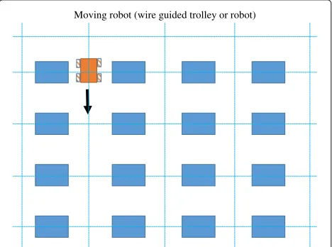
In many industrial production applications, such as in an indoor workshop, a set of devices is arranged in the indoor space, as shown in Fig. 1. The position of each device is precisely defined, and generally, these devices are regu-larly deployed on the ground following a certain rule. A robot is moving along the predefined lines in this work-ing space and will stop at one of the predefined positions to check each device. This scenario can be modeled as a grid as shown in Fig. 2, where we suppose that the mobile
Moving robot (wire guided trolley or robot)
Fig. 2Grid defining the possible positions
robot can only stop at one of the intersection dots of a grid. So the localization problem consists only in making a choice between the intersection points. The proposed technique, exploiting the a prior knowledge of the possible locations of the devices, allows localizing the robot in one of the intersection dots and tracking the trajectory of the robot and the variation of the channel parameters due to the changement of the environment. RSSI-based localiza-tion method is a good oplocaliza-tion for this specific applicalocaliza-tion but we have to check that:
(1) Errors due to the channel model inaccuracy are less than the grid resolution.
(2) Small position error correction is possible and can be used to track in real time the channel variations.
These two conditions will be developed later in the paper. Without loss of generality, we consider in this study that the size of the grid is 10 m×10 m. Anchors are placed on three dots, whose coordinates are (0, 0), (0, 10), (10, 0), respectively. In Fig. 2, 1 denotes 1 m. A reference node is placed in the center of this region, whose coordinate is (5, 5).
2.2 RSSI channel model
Model-based RSSI localization techniques have been pro-posed in the literature for different radio technologies. Among a number of channel models proposed for outdoor and indoor environments (Nakagami, Rayleigh, Ricean, etc.), the most popular channel model for RSSI-based localization, thanks to its simplicity, is the lognormal shadowing path loss model [30, 31], which expresses the
following relation between the received power and the transmitter-receiver distance:
RSSI(k,i)=Ak−10ηklog(dk)+v(k,i) (1)
wheredk is the distance from the unknown node to the kth anchor node,Ak andηk are the model parameters of
thekth anchor, andv(k,i)is a zero-mean white Gaussian
random variable with standard deviationσk. Suppose that the distance estimation is based onMsamples of RSSI(k,i),
which represents theith RSSI sample measured by thekth anchor node. For getting a good performance, the median value of RSSI(k,i)is used to obtain the distance estimate:
ˆ dk =10
Ak−RSSIk
10ηk (2)
where RSSIk, the median RSSI value measured by thekth
anchor, is given by:
RSSIk=Median
RSSI(k,i),i=1,· · ·,M
(3)
To characterize the RSSI model in an indoor environ-ment, measurements have been realized. The experiment has been done in a large hall. The testing scene is shown in Fig. 3. The experimental testbed has been build using three wifi access points (AP) and a mobile wifi point. The three wifi access points represent the three anchor nodes, and the mobile wifi point is considered as the unknown node.
To establish the practical channel model in this hall, many measurements have been performed on diffierent positions. In the measurement, to acquire a large number of RSSI values in each distance, we give a same distance value between each access point and the mobile point, for example 1 m. Then in the process of measurement, the mobile point is changed for 30 directions but its distance with the three APs is not changed. So, the mobile point receives 30 RSSI values from each AP, and 90 diffierent RSSI values are measured for distance 1 m. Repeating this
AP AP
Mobile point
AP
measurement process, a large number of RSSI data are obtained by changing the distance from 1 to 10 m with interval 0.5 m.
Based on the measured RSSI data, the median RSSI is calculated for one distance. Figure 4 presents the measured median RSSI as function of the distance. As expected, we can find that the median RSSI value decreases with the distance. From these results, we can deduce the following parameters in (1): Ak = −9.39,
ηk=2.27.
Meanwhile, the standard deviation of the noise for each distance can be estimated by:
ˆ
The obtained results are shown in Fig. 5. From the experimental results, the standard deviation of the noise, in terms of the distance from 1 to 10 m, can be expressed as:
σ (d)= −0.1108d2+2.1836d−0.3821 (6)
The variance model defined by (6) is of course specific to our measurement condition but indicates that the RSSI variance tends to increase with distance which has been already observed in some work [32]. It is worth noting that the relationship between the noise variance and distance depends on the environment size and complexity.
0 0.2 0.4 0.6 0.8 1
Fig. 4Relationship of measured RSSI values and distance
1 2 3 4 5 6 7 8 9 10
Fig. 5Relationship of the noise standard deviation and distance for measured data
2.3 Trilateration algorithm
The trilateration algorithm is a basic positioning method, widely used in many localization systems [33, 34]. In this algorithm, at least three anchor nodes are needed for positioning the target. The position of the anchor nodes is assumed to be known. The relationship between the unknown nodes position and three anchor node positions can be expressed as:
⎧ the coordinates of the three anchors. Equations (7) can be written into the following matrix form:
Qx=b (8)
whereQis a matrix of dimensionr×r,xis the coordinate vector,bis a vector of dimensionr, andris the dimension of position coordinates.
For two-dimensional problem considered in this study,
Qwith dimension 2×2 andbwith dimension 2 are written respectively as:
at (0, 0), (0, 10), (10, 0), respectively. Under this deploy-ment, it is easy to show that|Q| =0, thenQis invertible. Consequently, the estimated position is given by:
x=Q−1b=Pb where x=
ˆ x ˆ y
(11)
where (xˆ,ˆy) is the estimated position obtained by the trilateration method.
2.4 LMS method
LMS algorithm can be considered as a basic machine learning algorithm, widely used for parameter estimation [35]. LMS allows finding the values of parameters of a function after several iterative calculations in a computa-tionally efficient way [36]. It is based on approximating the true gradient of the squared error of estimation by its instantaneous estimate. In the proposed tracking strategy, the error is minimized by recursively modifyingAandη
of the channel model. As illustrated in Fig. 6, RSSI val-ues related to the three anchor nodes are acquired by the reference or target node. At each iterationt, the related distances are measured by (2) withA(t−1)andη(t−1)
estimated at iteration(t−1). Then, the trilateration algo-rithm calculates the estimated position(xˆ(t),yˆ(t)). With the known real position of reference point(x,y), the local-ization error is calculated as:
ε(t)=
(xˆ(t)−x(t))2+(ˆy(t)−y(t))2 (12)
wheretdenotes the iteration number.
This error serves as the input to the LMS algorithm, and by adaptively minimizing the localization error, we obtain
ηas follows:
η(t)=η(t−1)−μη
∂ε(t)2
∂η (13)
Similarly, we can getAfrom the following equation:
A(t)=A(t−1)−μA∂ε(t)
2
∂A (14)
whereμηandμAare the adaptation step sizes, which can
be adjusted experimentally. The detailed derivation pro-cess and related calculation equations are given in the Appendix.
2.5 Tracking strategy
The whole proposed tracking strategy and localization process are illustrated in Fig. 6. In the proposed algorithm, this task is done in two steps: an initial channel estimation using a reference node followed by a tracking proce-dure using a grid correction based on the constrained positions.
In the first step, the mobile robot is positioned at a reference point whose position is known. Then, the tri-lateration algorithm is used to estimate the location and LMS is employed to find the channel parametersAˆ andηˆ
which minimize the positioning error.
After the acquisition step, a grid correction strategy is adopted for the localization and channel variation track-ing. We subdivide this step into the following procedures. 1. Based onAˆandηˆobtained in the acquisition step, we estimate the unknown node position denoted by(xˆ,yˆ).
2. After getting(xˆ,yˆ), we calculate all the distance val-ues between(xˆ,yˆ)and the intersection points in the grid. The nearest intersection point will be selected as the most likely position, whose coordinates are(x˙,y˙).
3. Knowing the most likely position(x˙,y˙), we use LMS to track the space and time evolution of the channel parameters, the tracked parameters are denoted by A˙ andη˙.
4. These procedures can be repeated in real time. The process can be easily extended to a scenario where there are also non-anchor nodes in fixed positions that first localize themselves and then contribute to the track-ing.
3 Simulation and analysis 3.1 Localization results
After acquiring the channel model from the experimental data, we can assess the localization process using simu-lation. In the simulation, the unknown node position is randomly selected from the intersection points of the grid. Then, for each position we calculate the RMSE value of the estimated localization, defined as [37]:
RMSE= 1 T
T
t=1
(xˆ(t)−x(t))2+(yˆ(t)−y(t))2 (15)
where(x(t),y(t))is the actual selected position.(xˆ(t),yˆ(t))
is the position estimated by the trilateration method. T is the number of randomly chosen positions. In all the following simulations,Tis taken as 500.
As illustrated in Table 1, with the increase of sample number Mused to calculate the median RSSI value, the RMSE values of the estimated location decrease, which indicates that the accuracy of localization gets better. To guarantee the efficiency of the tracking strategy, in the fol-lowing tracking step and simulations, the sample number Mis set to 300.
3.2 Parameter convergence
In the acquisition step, the actual values ofAandηare −10 dBm and 2.24, respectively, and the initial values are −9 dBm and 2.28. As illustrated in Figs. 7 and 8, after the acquisition step, with the help of trilateration and LMS methods, we can obtainAvalue very close to−10 dBm. Similarly, the obtainedηvalue is very close to 2.24. Fur-thermore, in the tracking step, we suppose that the true value ofA is−11 dBm and the true value of ηis 2.20. In the same manner, we can get A value very close to −11 dBm andηvalue very close to 2.20, so the proposed strategy can track the variation of the parameters in the monitored region.
3.3 Limitation analysis
However, there exists a limitation in the grid correction. If the localization error is larger than the grid step size, it is no more guaranteed that the correction strategy will be efficient. Therefore, we need to analyze the relationship between the step size and parameter variation which gives us a criterion to choose an appropriate step size value.
As shown in Fig. 9, the real position(x(t),y(t))is located in the center. The distance from(x(t),y(t))to its four pos-sible nearest positions is equal to the grid step sizes. If the estimated position(x(t),y(t))is located in the dark region, we can get a right correction. This region is defined by the following relationships:
(x(t)−x(t))2< s42
(y(t)−y(t))2< s42 (16)
wheresis the step size.
If the localization error ε(t) < 2s, the estimated posi-tion (x(t),y(t)) is located inside the circle. We are sure that the grid correction strategy is effective and it guaran-tees a satisfactory position correction. In the simulation, we perform 1000 estimation iterations in the predefined
Table 1Localization accuracy
Sample number M 30 50 200 300 500 1000
RMSE (m) 0.78 0.56 0.33 0.25 0.14 0.10
0 50 100 150 200 250 300 350 400 450
2.18 2.2 2.22 2.24 2.26 2.28 2.3
N(localization times)
η
Fig. 7Convergence process ofη
region and find grid step sizeswhich meets the following probability relationship:
P
ε(t) < s
2
>0.95 (17)
We define the parameters variation: η and A between the acquisition step and tracking step as follows:
η= | ˙η− ˆη| A= | ˙A− ˆA| (18)
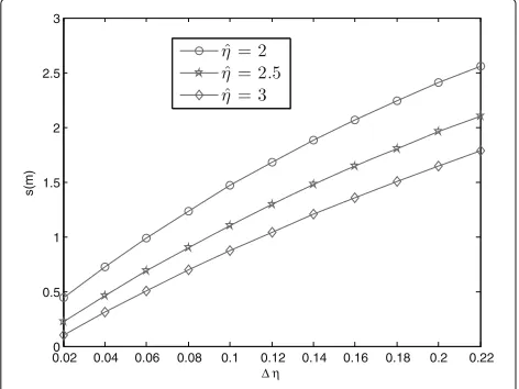
In the simulation, ηˆ is set to be 2.27 and η increases from 0.02 to 0.22 with interval 0.02. Similarly,Aˆ is set to be−9.39, andAincreases from 0.5 to 4 dB with inter-val 0.5 dB. The relationship betweensandηis shown in Fig. 10. With the increase ofη, the needed step size becomes larger and larger. According to these simulation results for three differentηˆ values, for a sameη value, the needed step size increases inversely withηˆ. When the value ofηis determined, we can find a threshold value of step sizesthreshold. As long assis larger thansthreshold,
0 50 100 150 200 250 300 350 400 450
−11.5 −11 −10.5 −10 −9.5 −9
N(localization times)
A(dBm)
Fig. 9Relationship of step size and localization error
we can get a right correction. Similarly, the relationship of step sizes andA is shown in Fig. 11. These results provide a criteria to guarantee that the proposed track-ing strategy is effective by maktrack-ing the trade-off between grid step sizesand parameter variation. In practice, the grid step size is fixed by the application, this calculation could give us a mean to make an alarm on the possible fail-ure of the tracking strategy by estimating the variation of parametersηandAin the monitored region.
3.4 Performance comparison
In this part, the localization performance of the proposed tracking strategy is compared with SDP [24] and WLS
0.020 0.04 0.06 0.08 0.1 0.12 0.14 0.16 0.18 0.2 0.22
0.5 1 1.5 2 2.5 3
Δ η
s(m)
Fig. 10Relationship betweensandη
0.5 1 1.5 2 2.5 3 3.5 4
0 1 2 3 4 5 6 7 8 9 10
Δ A(dB)
s(m)
Fig. 11Relationship betweensandA
[27] in terms of accuracy and computational complexity. The channel model parameters in (1) and the standard deviation of noise in (6) deduced from the experimen-tal data are used to provide RSSI values for assessing the compared algorithms. In the simulation, we suppose that the channel parameters are varying between the acqui-sition step and tracking step. In the proposed tracking strategy, the positioning is performed by trilateration after obtaining the tracked parametersA˙ andη˙. The number of iterations is set to be 50 for the proposed tracking strat-egy in these accuracy comparisons. In the simulation, the unknown node position is randomly selected from the intersection points of the grid, as illustrated in Fig. 2.
In the simulation,ηvaries from 0.004 to 0.04 with an interval of 0.004. As shown in Fig. 12, the RMSE value of the proposed method is noticeably smaller than that of SDP and WLS. WhenAvaries from 0.1 to 1.0 dB with an interval of 0.1 dB, the simulation results are shown in Fig. 13. Similarly, the proposed method exhibits better
0 4 8 12 16 20 24 28 32 36 40
0 0.5 1 1.5 2 2.5 3 3.5 4
Δ η
× 10−3
RMSE(m)
Proposed method WLS
SDP
Fig. 12Localization accuracy for three compared methods whenη
0.1 0.2 0.3 0.4 0.5 0.6 0.7 0.8 0.9 1.0 0.2
0.4 0.6 0.8 1 1.2 1.4 1.6 1.8 2
Δ A(dB)
RMSE(m)
Proposed method WLS
SDP
Fig. 13Localization accuracy for three compared methods whenA varies from 0.1 dB to 1.0 dB
performance than SDP and WLS. The simulation results show that SDP and WLS give low localization accuracy in case of parameter variation. In fact, the localization error increases withηandA, due to the increase in the esti-mated distance error. By inversing the channel model, the distance is estimated from (2). We can find that the esti-mated distance error increases with the increase of the variation of model parameters. So, the localization error also increases withη andA. Therefore, the SDP and WLS cannot provide good localization accuracy when the model parameters are changed. On the contrary, the pro-posed tracking strategy can track the parameters firstly and then perform the localization by trilateration. There-fore, the proposed method can give a higher accuracy.
In order to compare the computational complexity of the three methods, the execution time is evaluated by a computer with a processor unit (CPU) of 2.6 GHz and 16 GB of RAM. In the proposed method, the position is calculated by trilateration directly. So, the computational overhead is mainly due to the number of iterations in the tracking step. A larger iteration number will give a higher accuracy but more localization time. The relation between the tracking time and number of iterations is given in Table 2. It indicates that the tracking time increases with the number of iterations.
Based on the observation of parameters convergence process, the number of iterations in the tracking step is set to 50 in the performance comparison. The calculation time for three compared methods is shown in Table 3.
Table 2Relationship between tracking time and number of iterations
Number of iterations 30 50 80 100 150 200 300
Tracking time (s) 0.205 0.382 0.617 0.846 1.287 2.133 2.907
Table 3Calculation time for three compared methods
Method Proposed method SDP WLS
Average time (s) 0.384 0.032 0.024
The average time for a single localization of the proposed method is 0.384 s, while the corresponding values for SDP and WLS are 0.032 and 0.024 s, respectively. We can find that the proposed method requires more calculation time than SDP and WLS, due to the tracking step. More tracking iterations will cause more calculation time. The trade-off between the localization accuracy and the cal-culation time can be made according to the performance requirement.
3.5 Tracking test
In the tracking test, a large number of measurements have been done in the indoor hall as shown in Fig. 3. Firstly, the mobile point is placed on (5, 5). Position (5, 5) is considered as a reference point and 300 RSSI sam-ples are acquired in this position. Based on these RSSI data, the acquired parameter values areAˆ = −9.39 and
ˆ
η = 2.27. Hereafter, we placed the mobile point in posi-tions (6, 5), (7, 5), and (8, 5), and 300 RSSI values are acquired for each position. In the data collecting pro-cess, signal transmission path is changed by modifying the device direction or putting obstacles in the measurement scenario.
Based on the acquired RSSI data for each position, the estimated positions and tracked parameters by the pro-posed method are given in Table 4. As shown in Table 4, for position (6, 5), the estimated position is (6.12, 5.26). This estimated position meets the grid correction and tracking condition. By using LMS method, the tracked parameters are A˙ = −9.35 and η˙ = 2.26. Further-more, similar results are obtained for positions (7, 5) and (8, 5). These results show that the proposed tracking strat-egy can be effective. When the mobile point is moving from position (6, 5) to position (8, 5), parametersAandη
are changing. In this specific tracking test, the parameters variation is not very large. If the parameters are changing largely, the grid step size should be increased to guaran-tee the effectiveness of the proposed tracking strategy, as shown in Section 3.3.
Table 4Localization results and tracked parameters
Real position Estimated position A˙ η˙
(6, 5) (6.12, 5.26) -9.35 2.26
(7, 5) (6.98, 5.13) -9.41 2.28
4 Conclusions
In this paper, a RSSI-based parameter tracking strategy for constrained position localization is proposed. Median RSSI is calculated for distance estimation, and the tri-lateration algorithm is adopted to estimate the position. To track the variation of channel parameters, a novel tracking strategy with grid correction based on LMS is developed to obtain the actual parameters in the mon-itored indoor region. Based on practical data acquired from a real localization system, an experimental chan-nel model is constructed to evaluate the tracking strat-egy. The relationship between the localization accuracy and sample number of RSSI is discussed. The simulation results show the good behavior of the proposed track-ing strategy in presence of space-time variation of the propagation channel. To deal with the limitation of the proposed grid correction, the relationship between the grid step size and parameter variation is analyzed. Com-pared with the existing SDP and WLS, the proposed tracking strategy exhibits better localization accuracy but higher computational complexity. Moreover, the tracking test validates the effectiveness of the proposed tracking strategy.
Appendix
This appendix gives the detailed calculation process for LMS.
For parameterη, iterative calculation is given by:
η(t)=η(t−1)−μη
with respect toηare given by:
∂xˆ(t)
Similarly, the iteration equation onAis given by:
A(t)=A(t−1)−μA
with respect toAare given by:
∂xˆ(t)
AOA: Angle of arrival; AP: Access point; LLS: Linear least squares; LMS: Least mean squares method; NLS: Non-linear least squares; RMSE: Root mean square error; RSSI: Received signal strength indicator; SDP: Semidefinite
programming; TDOA: Time diffierence of arrival; TOA: Time of arrival; WSNs: Wireless sensor networks
Acknowledgements
The authors would like to thank the China Scholarship Council (No. 201406180059) for funding part of this work.
Funding Not applicable.
Availability of data and materials Not applicable.
Authors’ contributions
The authors declare equal contribution. All authors read and approved the final manuscript.
Ethics approval and consent to participate Not applicable.
Competing interests
The authors declare that they have no competing interests.
Publisher’s Note
Springer Nature remains neutral with regard to jurisdictional claims in published maps and institutional affiliations.
Received: 6 July 2017 Accepted: 30 October 2017
References
1. N Iliev, I Paprotny, Review and comparison of spatial localization methods for low-power wireless sensor networks. IEEE Sens. J.15(10), 5971–5987 (2015)
2. M Jamalabdollahi, S Zekavat, ToA ranging and layer thickness computation in nonhomogeneous media. IEEE Trans. Geosci. Remote Sens.55(2), 742–752 (2016)
3. JY Huang, Q Wan, Comments on “The Cramer-Rao Bounds of Hybrid TOA/RSS and TDOA/RSS Location Estimation Schemes”. IEEE Commun. Lett.8(10), 848–849 (2007)
4. S Tomic, M Beko, R Dinis, 3-D target localization in wireless sensor network using RSS and AoA measurements. IEEE Trans. Veh. Technol.6, 1–8 (2016) 5. D Niculescu, B Nath, inProceedings of Twenty-Second Annual Joint
Conference of the IEEE Computer and Communications. Ad hoc positioning
system (APS) using AOA (IEEE, San Francisco, 2003), pp. 1734–1743 6. J Velasco, D Pizarro, J Macias, A Asaei, TDOA matrices: algebraic properties
and their application to robust denoising with missing data. IEEE Trans. Signal Process.64(20), 5242–5254 (2016)
7. L Cong, W Zhuang, inProceedings of the IEEE International Conference on
Global Telecommunications. Non-line-of-sight error mitigation in TDOA
mobile location, vol. 1, (2001), pp. 680–684
8. P Abouzar, DG Michelson, M Hamdi, RSSI-based distributed
self-localization for wireless sensor networks used in precision agriculture. IEEE Trans. Wireless Commun.15(10), 6638–6650 (2016)
9. XR Li, RSS-based location estimation with unknown pathloss model. IEEE Trans. Wireless Commun.5(12), 3626–3633 (2006)
10. SY Han, NB Ghazaleh, D Lee, Efficient and consistent path loss model for mobile network simulation. Biol. Cybern.24(3), 1774–1786 (2016) 11. B Mukhopadhyay, S Sarangi, S Kar, inProceedings of Twenty First National
Conference on Communications (NCC). Performance evaluation of
localization techniques in wireless sensor networks using RSSI and LQI (IEEE, Mumbai, 2015), pp. 1–6
12. F Subhan, S Ahmed, K Ashraf, inProceedings of 16th International
Conference on Advanced Communication Technology. Extended Gradient
Predictor and Filter for smoothing RSSI (IEEE, Pyeongchang, 2014), pp. 1198–1202
13. G Oliva, S Panzieri, F Pascucci, R Setola, Sensor networks localization: extending trilateration via shadow edges. IEEE Trans. Autom. Control. 60(10), 12752–2755 (2015)
14. B Mukhopadhyay, S Sarangi, S Kar, inProceedings of Twentieth National
Conference on Communications (NCC). Novel RSSI evaluation models for
accurate indoor localization with sensor networks (IEEE, Kanpur, 2014), pp. 1–6
15. J Yin, Q Yang, L Ni, inProceedings of Third IEEE International Conference on
pervasive Computing and Communications, PerCom. Adaptive temporal
radio maps for indoor location estimation, (Hawaii, 2005), pp. 85–94 16. Y Gwon, R Jain, inProceedings of the Second International Workshop on
Mobility Management Wireless Access Protocols. Error characteristics and
calibration-free techniques for wireless LAN-based location estimation (ACM, Philadelphia, 2004), pp. 2–9
17. JY Zhu, AX Zheng, J Xu, K Li, inProceedings of International Conference on
Indoor Positioning and Indoor Navigation (IPIN). Spatio-temporal (S-T)
similarity model for constructing WIFI-based RSSI fingerprinting map for indoor localization (IEEE, Busan, 2014), pp. 678–684
18. D Moreas, L Felipe, B Astuto, inProceedings of the 4th ACM international
workshop on Mobility management and wireless access. Calibration-free
WLAN location system based on dynamic mapping of signal strength (ACM, Torremolinos, 2006), pp. 92–99
19. G Wang, K Yang, A new approach to sensor node localization using RSS measurements in wireless sensor networks. IEEE Trans. Wirel. Commun. 10(5), 1389–1395 (2011)
20. N Salman, AH Kemp, M Ghogho, Low complexity joint estimation of location and path loss exponent. IEEE Wirel. Commun. Lett.1(4), 5364–367 (2012)
21. RM Vaghefi, MR Gholami, RM Buehrer, EG Strom, Cooperative received signal strength-based sensor localization with unknown transmit powers. IEEE Trans. Signal Process.61(6), 1389–1403 (2013)
22. S Tomic, M Beko, R Dinis, Distributed RSS-based localization in wireless sensor networks based on second-order cone programming. Sensors. 14(10), 18410–18432 (2014)
23. A Coluccia, F Ricciato, RSS-based localization via Bayesian ranging and iterative least squares positioning. IEEE Commun. Lett.18(5), 873–876 (2014)
24. RW Ouyang, AK Wong, CT Lea, Received signal strength-based wireless localization via semidenite programming: noncooperative and cooperative schemes. IEEE Trans.Veh. Technol.59(3), 1307–1318 (2010) 25. S Tomic, M Beko, R Dinis, RSS-based localization in wireless sensor
networks using convex relaxation: noncooperative and cooperative schemes. IEEE Trans. Veh. Technol.64(5), 2037–2050 (2015)
26. N Salman, M Ghogho, AH Kemp, On the joint estimation of the RSS-based location and path-loss exponent. IEEE Wirel. Commun. Lett.1(1), 34–37 (2012)
27. G Wang, K Yang, On received-signal-strength based localization with unknown transmit power and path loss exponent. IEEE Wirel. Commun. Lett.1(5), 536–539 (2012)
28. P Tarrío, AM Bernardos, X Wang, JR Casar, inProceedings of International
Conference on Hybrid Artificial Intelligence Systems. Dynamic channel
model LMS updating for RSS-based localization (Springer, Wroclaw, 2011), pp. 127–135
29. P Tarrio, A Bernardos, J Casar, inPaper presented on International
Conference on Sensor Technologies and Applications, SensorComm. An RSS
localization method based on parametric channel models, (Valencia, 2007), pp. 265–270
30. D Madurasinghe, AP Shaw, Target localization by resolving the time synchronization problem in istatic radar systems using space fast-time adaptive processor. EURASIP J. Adv. Signal Process.16, 1–17 (2009) 31. TS Rappaport,Wireless Communications: Principles and Practice. (Prentice
hall PTR, New Jersey, 1996)
32. J Xu, W Liu, F Lang, Distance measurement model based on RSSI in WSN. Wirel. Sens. Netw.2(8), 606–616 (2010)
33. A Catovic, Z Sahinoglu, The Cramer-Rao bounds of hybrid TOA/RSS and TDOA/RSS location estimation schemes. IEEE Commun. Lett.8(10), 626–628 (2004)
34. QH Spencer, BD Jeffs, MA Jensen, AL Swindlehurst, Modeling the statistical time and angle of arrival characteristics of an indoor multipath channel. IEEE J. Sel. Areas Commun.18(3), 347–360 (2000)
35. P Tarrío, AM Bernardos, JR Casar, Weighted least squares techniques for improved received signal strength based localization. Sensors.11(9), 8569–8592 (2011)
36. V Mishra, G Chaitanya, inProceedings of Conference on IT in Business,
Industry and Government (CSIBIG). Analysis of LMS, RLS and SMI algorithm
on the basis of physical parameters for smart antenna (IEEE, Indore, 2014), pp. 1–4