Piecewise Linear Model-Based Image Enhancement
Fabrizio Russo
Department of Electrical, Electronic and Computer Engineering (DEEI), University of Trieste, Via Valerio 10, Trieste 34127, Italy
Email:[email protected]
Received 1 September 2003; Revised 23 March 2004
A novel technique for the sharpening of noisy images is presented. The proposed enhancement system adopts a simple piecewise linear (PWL) function in order to sharpen the image edges and to reduce the noise. Such effects can easily be controlled by varying two parameters only. The noise sensitivity of the operator is further decreased by means of an additional filtering step, which resorts to a nonlinear model too. Results of computer simulations show that the proposed sharpening system is simple and effective. The application of the method to contrast enhancement of color images is also discussed.
Keywords and phrases:image enhancement, sharpening, noise reduction, nonlinear filters.
1. INTRODUCTION
It is known that a critical issue in the enhancement of images is the noise increase that is typically produced by the sharp-ening process [1]. A classical example is represented by the linear unsharp masking (UM) method. Since a fraction of the high-pass filtered image is added to the original data, the resulting effect produces edge enhancement and noise am-plification as well. In order to address this issue, more eff ec-tive approaches resort to nonlinear filtering that can realize a better compromise between image sharpening and noise attenuation [2,3,4,5,6]. In particular, weighted medians (WMs) have been successfully experimented as a replace-ment for high-pass linear filters in the UM scheme [7]. In this framework, methods based on permutation weighted medi-ans (PWMs) offer very interesting results because they can prevent the noise amplification during the enhancement pro-cess [8,9]. Polynomial UM approaches constitute another family of nonlinear methods for image enhancement. Inter-esting examples include the Teager-based operator [10,11] and the cubic UM technique [12]. Rational UM [13] repre-sents a powerful approach to contrast enhancement. It can avoid noise amplification and excessive overshoot on sharp details. Nonlinear methods based on fuzzy models have also been investigated. Indeed, fuzzy systems are well suited to model the uncertainty that occurs when conflicting opera-tions should be performed, for example, detail sharpening and noise cancellation [14,15,16]. The most effective ap-proaches can enhance the image data without increasing the noise. However, their ability to reduce the noise during the sharpening process is limited. In this respect, methods based
on forward and backward (FAB) anisotropic diffusion con-stitute a powerful class of enhancement techniques [17,18]. Since anisotropic diffusion is typically an iterative process, the noise can be progressively reduced by means of an ap-propriate choice of parameter settings.
In this paper, a new simple technique for the enhance-ment of noisy images is presented. The proposed method improves our previous approach [19] from the point of view of architectural complexity and control of the nonlinear be-havior. The new algorithm adopts only one piecewise linear (PWL) function to combine the smoothing and sharpening effects. A two-pass implementation of the method is also pre-sented. As a result, noise reduction and edge enhancement can be achieved. This paper is organized as follows.Section 2
introduces a simple PWL model for image enhancement,
Section 3describes the complete two-pass enhancement ar-chitecture,Section 4shows results of computer simulations,
Section 5addresses parameter tuning,Section 6presents an application to color image processing, and finally,Section 7
reports conclusions.
2. A SIMPLE PWL MODEL FOR
IMAGE ENHANCEMENT
We suppose that we deal with digitized images having L gray levels. Let x(n) be the pixel luminance at location
n = [n1,n2] in the input image. The enhancement
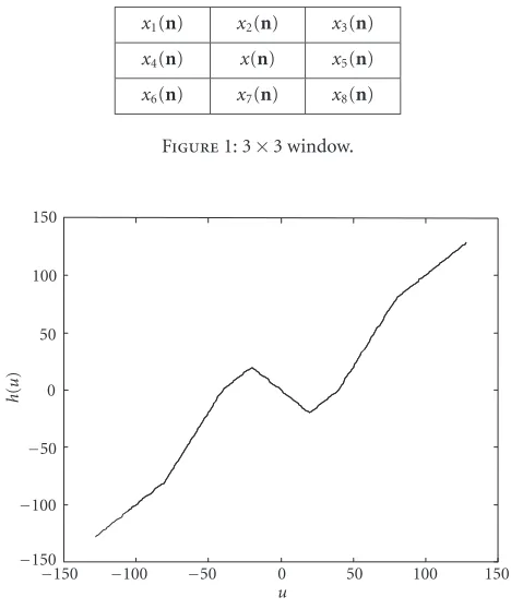
al-gorithm operates on a 3 × 3 window around x(n). Let
x1(n),x2(n),. . .,xN(n) briefly denote the group ofN = 8
neighboring pixels, as shown inFigure 1(0≤x(n)≤L−1;
x1(n) x2(n) x3(n)
Figure2: Example of graphical representation of functionh(u).
Let y(n) represent the output of the enhancement sys-tem. The algorithm is described by the following relation-ships: trolled by two parametersksmandksh:
h(u)=
An example of graphical representation ofh(u) is depicted in
Figure 2(ksm=20 andksh=2).
The basic idea is very simple. It takes into account the luminance differences∆xibetween the central pixel and its
neighbors (see (3)). When these differences are small, the method performs smoothing, that is, an action that aims at
reducing such differences in the enhanced image. Conversely, when the luminance differences are high, sharpening is pro-vided, that is, an effect that tends to increase such differences. According to (4), as|∆xi|increases, its effect in (2) becomes quite different. More precisely, this effect isstrong smoothing
for very small differences (|∆xi(n)|< ksm),weak smoothing
for small differences (ksm ≤ |∆xi(n)| <2ksm),strong sharp-eningfor medium differences (2ksm≤ |∆xi(n)|<4ksm), and weak sharpeningfor large differences (|∆xi(n)| ≥4ksm). The
shape of h(u) has been designed to gradually combine the smoothing and sharpening effects. The choice of a 7-segment model is based on experimentation. It is a compromise be-tween complexity and effectiveness. Models with more seg-ments require more parameters and do not yield a significant improvement. On the other hand, models with less segments do no provide enough performance and flexibility.
In our model, the actual amount of smoothing and sharpening can be controlled by the parametersksmandksh,
respectively. Whenksh=0, no sharpening is performed and
the resulting action is smoothing only. Thus (4) becomes
h(u)=
neighboring pixels are close to the value of the central ele-ment and we haveh(∆xi(n))= −∆xi(n). Thus, according to (1) and (2), the filter realizes the arithmetic mean of the pixel luminances in the neighborhood and the resulting effect is a strong smoothing action:
The filtering process aims at excluding luminance values
xi(n) that are very different from x(n) in order to avoid blurring the image details. According to this rule, when
|∆xi(n)| ≥ 2ksm, we haveh(∆xi(n)) = 0. A gradual
tran-sition betweenh(∆xi(n)) = −∆xi(n) andh(∆xi(n)) = 0 is
provided whenksm ≤ |∆xi(n)| < 2ksm (see (5)). As
above-mentioned, the smoothing behavior is controlled by the pa-rameter ksm. Large values ofksm increase the noise
cancel-lation, while small values increase the detail preservation. Notice that smoothing requires that h(∆xi(n)) < 0 when
∆xi(n)>0 andh(∆xi(n))>0 when∆xi(n)<0.
Now, we introduce the sharpening action. If we choose
ksh > 0 (typically ksh ≤ 6), a sharpening effect is applied
to the image pixels when |∆xi(n)| > 2ksm (see (4)). Since
sharpening can be considered as the opposite of the smooth-ing action [14,15], we seth(∆xi(n))>0 when∆xi(n)>2ksm
andh(∆xi(n))<0 when∆xi(n)<−2ksm. In particular, this
sharpening effect is stronger if 2ksm ≤ |∆xi(n)|<4ksmand
slope of the graph inFigure 2). This choice aims at avoiding an annoying excess of sharpening along the object contours of the image.
3. IMPROVING THE ENHANCEMENT PROCESS
The quality of the enhanced image can be improved by intro-ducing a further processing step for the cancellation of pos-sible outliers still remaining in the image. If the image is cor-rupted by Gaussian noise, these outliers typically represent the fraction of noise located on the “tail” of the Gaussian dis-tribution. Even if the probability of occurrence of these out-liers is low, their presence can be rather annoying, especially in the uniform regions of the image. The processing scheme described by (1), (2), (3), and (4) would require a large value of ksm to smooth out this kind of noise and, as a
conse-quence, some blurring of fine details could be produced. A more suitable choice is the adoption of an additional filtering step devoted to the cancellation of these outliers. This choice permits us to use a smaller value ofksmthat can
satisfacto-rily preserve the image details. The filter for outlier removal adopts a different approach to process the luminance diff er-ences in the window. Indeed, the filter aims at detecting pixel luminances that are very different from those of the neigh-borhood. The filter is defined by the following relationship:
y(n)=x(n)− MIN
i=1,2,...,N
g∆xi(n) + MINi
=1,2,...,N
g−∆xi(n) ,
(7)
wheregis a nonlinear function:
g(v)=
v, 0< v≤L−1,
0, v≤0. (8)
The shape of functiong is chosen to achieve the exact cor-rection in the ideal case of an outlier in a uniform neighbor-hood. As an example, letx(n)=abe a positive outlier and letxi(n)=b(i=1, 2,. . .,N) be the luminance values of the
neighboring pixels (a > b). Since∆xi(n)=a−b >0, we have
g(∆xi(n))=a−bandg(−∆xi(n))=0. Thus (7) yields the
exact valuey(n)=b. The filtering action defined by (7) and (8) can be applied after the sharpening process in order to re-move outliers. A better choice, however, is to apply this filter-ing to the noisy input data before the enhancement process, thus avoiding amplification of these outliers. The influence of the different parameter settings and processing strategies can be highlighted by some application examples.Figure 3a
shows a synthetic test image and Figure 3b the same pic-ture corrupted by Gaussian noise with variance 50. The re-sult of the application of our method (ksm = 10,ksh = 5)
without additional processing is reported in Figure 3c. The presence of many outliers is apparent. A larger value ofksm
can smooth out this noise as shown inFigure 3d(ksm =20, ksh =5). If fine details were present in the image, however,
this choice would produce some blurring. The result yielded by the improved enhancement process adopting additional filtering are depicted in Figure 3e(postfiltering, ksm = 15,
(a) (b)
(c) (d)
(e) (f)
Figure3: Details of (a) a synthetic image, (b) image corrupted by Gaussian noise with variance 50, (c) enhanced image (ksm =10,
ksh=5, no additional processing), (d) enhanced image (ksm=20,
ksh=5, no additional processing), (e) enhanced image (ksm=15,
ksh=5, postprocessing), and (f) enhanced image (ksm=15,ksh=
5, preprocessing).
ksh = 5) andFigure 3f (prefiltering, ksm = 15, ksh = 5).
We can observe that the latter gives the best result. As above mentioned, the smoothing action can easily be controlled by varying the value ofksm. A suitable choice can realize a
com-promise between noise cancellation and preservation of fine details and textures.
4. RESULTS
(a) (b)
(c) (d)
(e) (f)
(g)
Figure4: (a) Original image, (b) noisy image, (c) results given by linear UM, (d) WM UM, (e) PWM-UM, (f) FAB anisotropic diff u-sion, and (g) proposed method.
Figure 4c. (We setλ=0.4, whereλis the tuning parameter that defines the amount of sharpening.) We can observe that the noise increased significantly as an effect of the sharpening action and the result is very annoying. A better result is of-fered by the nonlinear UM based on the WM (Figure 4d,
λ = 0.5). However, its sensitivity to noise is rather high. Nonlinear UM based on PWMs represents a much powerful
choice (Figure 4e). We considered the algorithm that allows thresholding (L = 2,λ = 0.8,T = 50) [9]. Observing the image inFigure 4e, basically, no noise amplification is per-ceivable with respect to the input data.
An excellent combination of smoothing and sharpening is given by FAB anisotropic diffusion. We chose the algorithm that adopts the Gaussian-shaped function for the conduction coefficient and the following parameter settings:β1(1)=50, β2(1) =300,γ =0.5, and number of passes=3 [18]. The
corresponding result is shown in Figure 4f. Finally, the im-age yielded by our technique adopting preprocessing is rep-resented inFigure 4g(ksh =5,ksm =15). The good
perfor-mance in reducing noise is apparent. The processed picture looks almost noiseless and the edges are sharply reproduced. From the point of view of the image quality, the results given by our method and the FAB anisotropic diffusion are compa-rable. However, our method requires the choice of a smaller number of parameters. This is a key advantage of the pro-posed approach. In order to appraise the nonlinear behav-ior of the different sharpeners, the luminance values of a row are graphically depicted inFigure 5. The original noise-free row number 275 (from top to bottom) is shown inFigure 5a. The corresponding row in the noisy picture is represented in Figure 5b. The significant noise increase yielded by lin-ear UM is highlighted in Figure 5c. As above-mentioned, a smaller noise increase is produced by the nonlinear UM scheme based on the WM (Figure 5d). The result given by the PWM sharpener is shown inFigure 5e. According to our previous observation, the processed data remains as noisy as the input data, and no noise amplification is produced. The data processed by FAB anisotropic diffusion and by our method are depicted in Figures 5fand5g, respectively. We can easily notice that, unlike the other techniques, the noise has been reduced (for a comparison, look at the noise-free data inFigure 5a).
0 100 200 300 400 500 Pixel location in the row
Lu
Pixel location in the row
L
Pixel location in the row
L
Pixel location in the row
L
Pixel location in the row
L
Pixel location in the row
L
Pixel location in the row
L
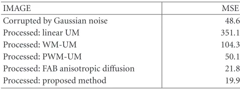
Table1: MSE values (Gaussian noise).
IMAGE MSE
Corrupted by Gaussian noise 48.6
Processed: linear UM 351.1
Processed: WM-UM 104.3
Processed: PWM-UM 50.1
Processed: FAB anisotropic diffusion 21.8
Processed: proposed method 19.9
Table2: MSE values (uniform noise).
IMAGE MSE
Corrupted by uniform noise 79.7
Processed: linear UM 213.1
Processed: WM-UM 105.7
Processed: PWM-UM 80.3
Processed: FAB anisotropic diffusion 76.6
Processed: proposed method 75.9
Processed: FAB anisotropic diffusion 31.7
Processed: proposed method 31.8
We measured the performance by using the peak signal-to-noise ratio (PSNR), which is defined as follows:
PSNR=10 log10
wherev(n) denotes the luminance value of the original image at pixel locationn =[n1,n2]. The list of PSNR values given
by the different methods is reported inTable 3. The good per-formance of our simple technique is apparent. The two-pass algorithm is written in C language. Look-up tables (LUTs) are currently adopted for implementing the PWL functions in order to speed up the processing. As a result, the algorithm typically requires 25 milliseconds to process a 256×256 im-age on a 2.6 GHz Pentium IV-based PC.
5. PARAMETER TUNING
As above-mentioned, the key feature of our technique is the combination of effectiveness and simplicity. Indeed, the choice of parameter valueskshandksmis a very easy process
because the nonlinear behavior is not very sensitive to them. A heuristic procedure starts by choosing a suitable value of
ksh(typically 4≤ksh≤6) and operates by varyingksmfrom
zero to a value that yields a compromise between noise re-duction and detail preservation. We consider some applica-tion examples.
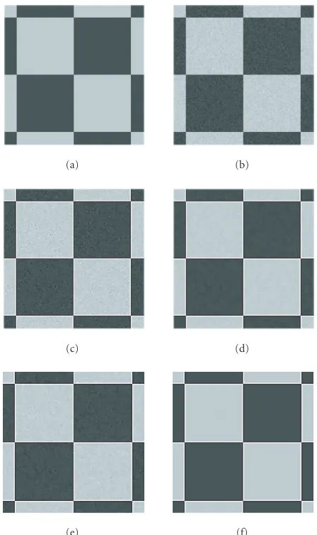
For the sake of simplicity, let the input image be an orig-inal (noise-free) picture as depicted inFigure 6a. The activa-tion of sharpening only (ksh =5,ksm =0) produces some
noise increase (Figure 6b). This effect can be corrected by ac-tivating the smoothing action (ksh=5,ksm=5) as shown in Figure 6c. The choice ofkshis not critical. If we chooseksh=
6, the sharpening increase is limited (Figure 6d). Clearly, larger values ofkshproduce a stronger sharpening effect that
can become annoying as shown in Figure 6e (ksh = 10, ksm=5) andFigure 6f(ksh=15,ksm=5).
The different case of a blurred image is examined in
Figure 7a. A very small increase of the noise is perceivable after sharpening withksh=5 andksm=0 (Figure 7b). Thus,
a very limited smoothing suffices to correct this effect, as de-picted inFigure 7c(ksh=5,ksm=1). A small increase ofksh
is not critical (Figure 7d:ksh=6,ksm=1). Of course, larger
values ofksh increase the sharpening action, as represented
in Figure 7e(ksh = 10,ksm = 1) and Figure 7f(ksh = 15,
ksm=1).
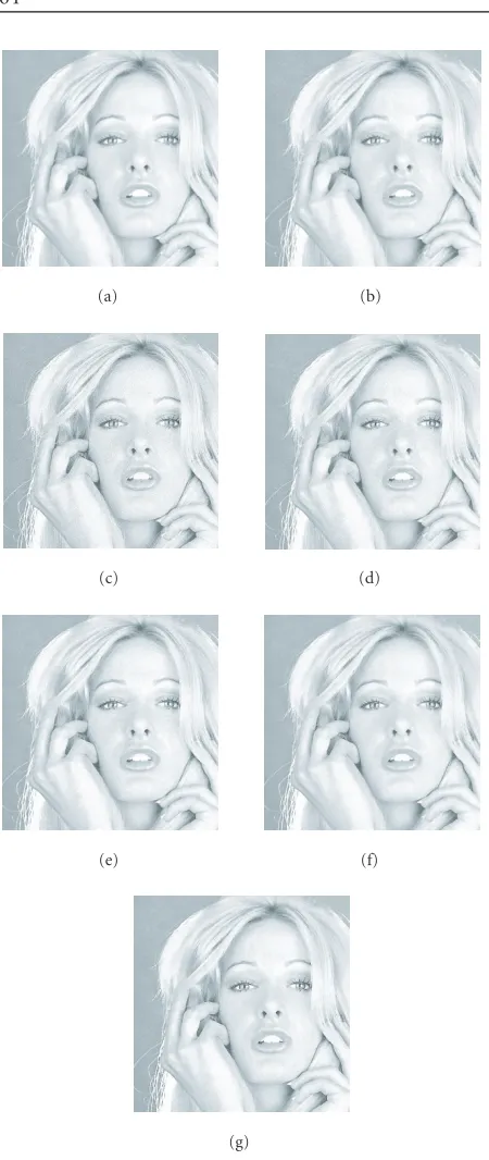
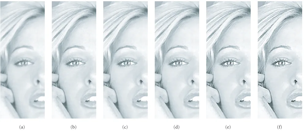
Finally, we consider a noisy input image.Figure 8ashows a detail of the picture represented inFigure 4b. In this case, a strong noise increase is produced after the enhancement withksh = 5 andksm = 0 (Figure 8b). Small values ofksm
do not suffice to correct this effect as shown in Figure 8c
(ksh = 5, ksm = 5) and Figure 8d (ksh = 5, ksm = 10).
A more effective smoothing is necessary in order to reduce the noise, as depicted inFigure 8e(ksh =5,ksm = 15). Of
course, too large values ofksmproduce an excess of
smooth-ing that yields some detail blur (Figure 8f:ksh=5,ksm=20).
This behavior can be taken into account in order to choose the set of optimal parameters for different types of pictures. If the image is rich in very fine details, small values of ksm
can represent a suitable choice. Conversely, if the picture is mainly composed of uniform regions, where the presence of noise is more annoying, the adoption of (slightly) larger values ofksm can provide a better smoothing effect. In this
case, the value of ksh can be reduced in order to avoid an
excess of noise increase. In this respect, an interesting im-provement would be the development of an adaptive pro-cessing approach, where different parameter values are used for different pixels depending on local features. An adaptive method based on the edge gradient of the image could in-crease the value ofksmin the uniform regions and then
per-form a stronger noise cancellation. On the contrary, smaller values of ksm (and, possibly, larger values ofksh) could be
adopted in presence of image details in order to improve the sharpening effect. Such an approach, whereksh andksm
de-pend on the edge gradient of the image, is a subject of present investigation.
6. APPLICATION TO COLOR IMAGES
(a) (b) (c) (d) (e) (f)
Figure6: (a) Detail of original noise-free image, and results given by different parameter settings: (b)ksh=5 andksm=0, (c)ksh=5 and
ksm=5, (d)ksh=6 andksm=5, (e)ksh=10 andksm=5, and (f)ksh=15 andksm=5.
(a) (b) (c) (d) (e) (f)
Figure7: (a) Detail of blurred image, and results given by different parameter settings: (b)ksh=5 andksm=0, (c)ksh=5 andksm=1, (d)
ksh=6 andksm=1, (e)ksh=10 andksm=1, and (f)ksh=15 andksm=1.
and consists in processing just the luminance component. An example is reported inFigure 9. We considered the original 24-bit color picture “Tiffany” and we generated a noisy im-age by adding zero-mean Gaussian noise with variance 50 to the R, G, and B components (Figure 9a). Then, we adopted the YIQ color space representation [20] and we processed the luminance Y component only. The resulting image given by our method is shown inFigure 9b.
7. CONCLUDING REMARKS
compro-(a) (b) (c) (d) (e) (f)
Figure8: (a) Detail of noisy image, and results given by different parameter settings: (b)ksh=5 andksm=0, (c)ksh=5 andksm=5, (d)
ksh=5 andksm=10, (e)ksh=5 andksm=15, and (f)ksh=5 andksm=20.
(a) (b)
Figure9: (a) Noisy 24-bit color image and (b) result of the applica-tion of the proposed method.
mise between detail sharpening and noise cancellation can be achieved. The quality of the enhanced data is improved by adopting a preprocessing step that avoids sharpening of possible outliers. The nonlinear behavior of this smoothing process is based on a different PWL model that performs a complementary action with respect to the other one.
Computer simulations have shown that the method yields very satisfactory results and that the parameter tuning is a very easy process. The method is also computationally light. As a result, potential applications to digital cameras, videocameras, and video cellular telephones can be devised.
ACKNOWLEDGMENTS
This work was supported by the University of Trieste, Italy. The source of the original images (Figures 4 and9) is the USC-SIPI Image Database (Signal and Image Processing In-stitute, University of Southern California).
REFERENCES
[1] A. K. Jain,Fundamentals of Digital Image Processing, Prentice-Hall, Englewood Cliffs, NJ, USA, 1989.
[2] G. Ramponi, “Polynomial and rational operators for image processing and analysis,” inNonlinear Image Processing, S. K. Mitra and G. Sicuranza, Eds., pp. 203–223, Academic Press, San Diego, Calif, USA, 2001.
[3] G. R. Arce and J. L. Paredes, “Image enhancement and analysis with weighted medians,” inNonlinear Image Processing, S. K. Mitra and G. Sicuranza, Eds., pp. 27–67, Academic Press, San Diego, Calif, USA, 2001.
[4] S. C. Matz and R. J. P. de Figueiredo, “A nonlinear tech-nique for image contrast enhancement and sharpening,” in
Proc. IEEE Int. Symp. Circuits and Systems (ISCAS ’99), vol. 4, pp. 175–178, Orlando, Fla, USA, May–June 1999.
[5] R. J. P. de Figueiredo and S. C. Matz, “Exponential nonlin-ear Volterra filters for contrast sharpening in noisy images,” inProc. IEEE Int. Conf. Acoustics, Speech, Signal Processing (ICASSP ’96), vol. 4, pp. 2263–2266, Atlanta, Ga, USA, May 1996.
[6] A. Polesel, G. Ramponi, and V. J. Mathews, “Image enhance-ment via adaptive unsharp masking,”IEEE Trans. Image Pro-cessing, vol. 9, no. 3, pp. 505–510, 2000.
[7] M. Fischer, J. L. Paredes, and G. R. Arce, “Weighted median image sharpeners for the World Wide Web,”IEEE Trans. Im-age Processing, vol. 11, no. 7, pp. 717–727, 2002.
[8] R. C. Hardie and K. E. Barner, “Extended permutation filters and their application to edge enhancement,” IEEE Trans. Im-age Processing, vol. 5, no. 6, pp. 855–867, 1996.
[9] J. L. Paredes, M. Fisher, and G. R. Arce, “Image sharpening using permutation weighted median filters,” inProc. Euro-pean Signal Processing Conference (EUSIPCO ’00), Tampere, Finland, September 2000.
Image Processing, S. K. Mitra and G. Sicuranza, Eds., pp. 167– 202, Academic Press, San Diego, Calif, USA, 2001.
[12] G. Ramponi, N. Strobel, S. K. Mitra, and T.-H. Yu, “Nonlinear unsharp masking methods for image contrast enhancement,”
Journal of Electronic Imaging, vol. 5, no. 3, pp. 353–366, 1996. [13] G. Ramponi and A. Polesel, “Rational unsharp masking tech-nique,” Journal of Electronic Imaging, vol. 7, no. 2, pp. 333– 338, 1998.
[14] F. Russo and G. Ramponi, “Fuzzy operator for sharpening of noisy images,” Electronics Letters, vol. 28, no. 18, pp. 1715– 1717, 1992.
[15] F. Russo and G. Ramponi, “Nonlinear fuzzy operators for im-age processing,”Signal Processing, vol. 38, no. 3, pp. 429–440, 1994.
[16] F. Russo and G. Ramponi, “An image enhancement technique based on the FIRE operator,” inProc. IEEE International Con-ference on Image Processing (ICIP ’95), vol. 1, pp. 155–158, Washington, DC, USA, October 1995.
[17] M. Black, G. Sapiro, D. Marimont, and D. Heeger, “Robust anisotropic diffusion and sharpening of scalar and vector im-ages,” inProc. IEEE International Conference on Image Process-ing (ICIP ’97), vol. 1, pp. 263–266, Santa Barbara, Calif, USA, October 1997.
[18] B. Smolka, M. Szczepanski, K. N. Plataniotis, and A. N. Venet-sanopoulos, “Forward and backward anisotropic diffusion fil-tering for color image enhancement,” inProc. 14th IEEE In-ternational Conference on Digital Signal Processing (DSP ’02), vol. 2, pp. 927–930, Santorini, Greece, July 2002.
[19] F. Russo, “An image enhancement technique combining sharpening and noise reduction,” IEEE Trans. Instrumenta-tion and Measurement, vol. 51, no. 4, pp. 824–828, 2002. [20] I. Pitas, Digital Image Processing Algorithms and Applications,
John Wiley & Sons, New York, NY, USA, 2000.
Fabrizio Russo obtained the Dr.-Ing. de-gree in electronic engineering (with the highest honors) in 1981 from the University of Trieste, Trieste, Italy. In 1984, he joined the Department of Electrical, Electronic and Computer Engineering (DEEI) of the Uni-versity of Trieste, where he is currently an Associate Professor of electrical and elec-tronic measurements. His main interests are in the field of nonlinear signal processing