Autoregressive modeling of transfer functions in frequency domain to determine
complex travel times
Yoko Hasada1, Hiroyuki Kumagai2∗, and Mineo Kumazawa3
1Department of Earth and Planetary Sciences, Nagoya University, Nagoya, Japan 2Research Center for Seismology and Volcanology, Nagoya University, Nagoya, Japan
3Tono Geoscience Center, Toki, Japan
(Received January 14, 2000; Revised August 20, 2000; Accepted September 11, 2000)
We present a method to determine the complex travel times of impulses in the time domain on the basis of an autoregressive (AR) modeling of superimposed sinusoids in a finite complex series in the frequency domain. We assume that the complex frequency series consists of signals represented by a complex AR equation with additional noise. The AR model in the frequency domain corresponds to a complex Lorentzian in the time domain. In a similar way to the Sompi or extended Prony method, the complex travel times are given by solutions of a characteristic equation of complex AR coefficients, which are obtained as the eigenvector corresponding to a minimum eigenvalue in an eigenvalue problem of non-Toeplitz autocovariance matrix of the complex series. Our method is tested for synthetic frequency series of transfer functions, which show that (1) the complex travel times of closely adjacent pulses in the time domain are clearly resolved, and that (2) the frequency dependence of the complex travel times for physical and structural dispersions is precisely determined by the analysis within a narrow frequency window. These results demonstrate the usefulness of our method with high resolvability and accuracy in the analysis of impulse sequences.
1.
Introduction
The conversion of superimposed sinusoids in the time do-main to a set of spectral peaks in the frequency dodo-main is usually called the spectral analysis. There are two types of approach for spectral analysis: one is transformation such as the Fourier transform, and the other is a modeling in which the input data is fitted to an a priori model such as the autoregres-sive (AR) or autoregresautoregres-sive and moving average (ARMA) model. There are many different spectral analysis methods based on modeling (see e.g. Kay and Marple, 1981).
Our present concern is the conversion by a modeling of superimposed sinusoids in the frequency domain to a set of peaks indicating events such as the arrival of pulses in the time domain. A proposed approach in this paper is based on the AR process model represented by the Prony’s rela-tion (see Hildebrand, 1956). Among many different types of the extension (Pisarenko, 1972; Price, 1979; Chao and Gilbert, 1980, etc.), we use the particular one called the Sompi method (e.g. Hori et al., 1989; Kumazawa et al., 1990), in which unbias estimations of model parameters are made by using an eigenvalue problem of non-Toeplitz au-tocovariance. Our approach determines a set of oscillation “frequency” in the complex frequency series of transfer func-tion. The oscillation “frequency” represents the arrival time
∗Now at National Research Institute for Earth Science and Disaster Pre-vention, Tsukuba, Japan.
Copy right cThe Society of Geomagnetism and Earth, Planetary and Space Sciences (SGEPSS); The Seismological Society of Japan; The Volcanological Society of Japan; The Geodetic Society of Japan; The Japanese Society for Planetary Sciences.
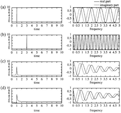
of impulse waves (Fig. 1). We assume that the complex dis-crete frequency series consists of signal and noise, where the signal is represented by a complex AR equation. The travel time is defined as a complex value whose real and imaginary parts correspond to the time delay and pulse width, respec-tively. The complex travel time is determined in a similar way to the Sompi method. Accordingly, we introduce con-cepts of the complex time and the aliasing in the time domain for our analysis.
The concept of converting frequency sequence to a set of time-localized events has been already popular in terms of “cepstrum” for echo analysis (Bogartet al., 1963), and extensive studies have been made (see e.g. Childers et al., 1977). As far as this point is concerned, our method is a kind of the cepstrum modeling approach. Whereas the cepstrum analysis appears merely as an inverse operation to spectrum analysis, historical development of the cepstrum theory fol-lowed a considerably different way: The cepstrum has been a theoretically well established concept categorized as one of the homomorphic transformations in widely known text-books (e.g. Oppenheim and Schafer, 1975).
The present method is developed for analyzing a finite dis-crete frequency series data of the transfer function acquired by a new structural exploration system named ACROSS (Accurately-Controlled Routinely-Operated Signal System, e.g. Kumazawa and Takei, 1994) and by laboratory studies for the measurement of sound velocities in the frequency domain (e.g. Shanklandet al., 1993). Whereas the inverse Fourier transform was used in Shanklandet al.(1993), we introduce the AR modeling approach as a better alternative.
Fig. 1. The impulse response functions (left) and the corresponding transfer functions in the frequency domain (right) for a non-dispersive medium without attenuation ((a) and (b)) and with attenuation ((c) and (d)). The impulse response functions in (c) and (d) is the real part of the complex Lorentzian withφ=0 for (c) andφ=π/4 for (d) in Eq. (8), respectively.
In this paper, we present (1) the basic concept and theory of our method, and (2) results of numerical tests based on synthetic frequency series of transfer functions. In these tests, we show that our method determines arrival time as well as pulse width with high accuracy and resolvability, which is particularly powerful for dispersion analysis.
2.
Theory
2.1 Model of a sequence of impulses
Suppose that a time-localized signal (impulse) f0(t) lo-cated at x = 0 andt = 0 is propagated through a certain medium to a certain observation point. The original impulse may split into different modes of waves, each of them prop-agating in different paths to reach the observation point, and the observed signal f(t)may consist of afinite number of modified impulses or wavelets due to propagation;
f(t)=
l
αlf0(t−ql), (1)
whereαlandqlare the amplitude and time delay oflth pulse,
respectively.
First, we discuss how the time delay ql is generated by
wave propagation in a homogeneous medium. The propaga-tion of a wave with angular frequencyωfromt =0 to the point located at the distancexis generally described as
αeiωt−i kx =αeiω(t−kωx),
whereαis the amplitude at the origin andkis the wavenumber for a wave averaged over its propagation path. The time delay qdefined for a single frequency is given by
q = x
c, (2)
wherec = ω/k is the phase velocity given by the wave-numberk. When the medium is dissipative, the phase veloc-ity is the complex valuec˜defined as
1 ˜
c =
1 c
1− i 2Q
,
whereQ−1is the attenuation factor. Accordingly, we define q as the complex quantity,
q =τ+iυ, (3)
where
τ = x c
υ = − x 2c Q.
Our primary model for an impulse sequence is f(t)in Eq. (1), which is generated from a single impulse f0(t) con-taining different frequency components. The Fourier trans-form of Eq. (1) is written as
F(ω)=F0(ω)
l
αle−i qlω, (4)
whereF0(ω)is the Fourier transform of f0(t). The transfer function in the frequency domain is defined by
H(ω)= F(ω) F0(ω) =
l
αle−i qlω. (5)
Here, we propose an impulse model corresponding to Eq. (5). The inverse Fourier transform of H(ω)in Eq. (5) leads to
h(t)= 1
π
l
Re
iαl
t−ql
= π1
l
Re [Ll(t)], (6)
which describes a set of polesql located in the complext
space. The real part ofqlrepresents the arrival time, and the
imaginary part is related to the pulse widthwl through the
relation,
wl = −2υl. (7)
The time-dependent functionLl(t)in Eq. (6) has central
importance in the present method, so that we examine its property below. We refer to L(t)as a complex Lorentzian, which is a function of complex time,
L(t)= iα
t−q, (8)
whereαis the complex amplitude defined asα=α0eiφ. The real and imaginary parts ofL(t)are written as
Re[L(t)] Im[L(t)]
= α0
(t−τ)2+υ2
cosφ−sinφ sinφ cosφ
−υ
t−τ
.
0, whereas the imaginary part is asymmetric function with respect tot =τ. Either part is a linear combination of the symmetric and asymmetric components for a general value ofφ(Fig. 1). Therefore, asymmetric factor is incorporated into this impulse model. An asymptotic limit ofL(t)is the delta function att=τ;
lim
υ,φ→0Re[L(t)]=α0δ(t−τ).
In the model described above, each pulse has long tails extending indefinitely to±∞that appear to violate causality. It is necessary for the dispersion in an attenuating medium to satisfy causality (see e.g. Aki and Richards, 1980). This problem will be discussed below.
2.2 Model of dispersive wave
Here, we consider a homogeneous dispersive medium, in which the wavenumber is a frequency-dependent complex valuek˜(ω). The transfer function in Eq. (5) is expressed as
H(ω)=
l
αle−ik˜l(ω)xl, (9)
wherexl is the distance from the source. Althoughk˜l(ω)
is a function of the frequency for a dispersive medium, the extent of frequency dependence is usually weak. Therefore,
˜
kl(ω)can be expanded into a Taylor series around a particular
frequencyω=ω0up to thefirst order,
Inserting Eq. (10) into (9), we have
H(ω)=
l α
le−
i qlg(ω0)(ω−ω0) (11)
whereαlis the complex amplitude given by
α
whereu˜lis a complex group velocity,
1
andQgl is the quality factor related to the group velocity. Apparently, any time sequence consisting of delayed sig-nals is represented by a superposition of sinusoids in the frequency domain in a narrow frequency range, even if each of the signals is no longer a time-localized wavelet. In other words, Eq. (11) is applied even for long wave trains gener-ated from an impulse after propagating in a highly dispersive medium, for example. This is an important aspect in the present method.
Here, we introduce H(ω0, ω) as the transfer function within a narrow frequency band aroundω0,
H(ω0, ω)=
We have three expressions for a transfer function, Eqs. (5), (11), and (14); Eq. (5) is a general expression in terms of phase delay, whereas Eqs. (11) and (14) are general expres-sions in terms of group delay at the frequencyω0. The phase delay and group delay are equal for non-dispersive media, andαl = βl(ω0). Taking the dispersion into account, the impulse sequence model represented by the complex Lor-entzian shown in Eq. (6) is considered as that viewed within a narrow frequency band. Each of the poles in Eq. (6) is a
“wave element”characterized by two complex quantities,α andq, both being a function of frequency f0=ω0/2π. The quantityq, referred to as“complex delay”in Kay and Marple (1981), is defined as“complex travel time”: Its real partτ gives the delay time or travel time of group velocity and the imaginary partυ the attenuation characteristics for a wave element within the narrow frequency band around f = f0.
2.3 Model of observed frequency series and determina-tion of AR coefficients
We model afinite complex discrete series of H(ω) con-sisting of the decaying (or growing) sinusoids in a similar way to the Sompi or extended Prony method to determine a set of complex travel times and amplitudes. We extend the theory of the Sompi method to the analysis of the complex series.
We assume that an observedfinite discrete complex fre-quency series {Xj}consists of the signal{Hj}, which is a finite complex discrete series ofH(ω), and noise{Ej}:
Xj =Hj+Ej (j=1, . . . ,N) (15)
where {Ej}is a complex sequence of the Gaussian white
noise assumed to have zero mean and variance σ2. The signal {Hj} satisfies the following homogeneous complex
AR equation,
, which is related to the complex travel timeqas,
z=e−i2πqΔf (18)
To determine the complex AR coefficients{al}, we
mini-mize thefitting error
F = 1
with a constraint for obtaining non-zeroal,
M
l=0
alal∗ =1, (20)
where * denotes the complex conjugate. The factorFdefined in Eq. (19) corresponds to the noise power,
F = 1
Minimization of Eq. (19) under the condition Eq. (20) is solved by the Lagrangian undetermined multiplierλ,
∂
This leads to the eigenvalue problem,
M
Here, note that Pml is a non-Toeplitz Hermitian
autocovari-ance matrix.
The complex AR coefficientalcan be determined by
solv-ing the eigenvalue problem of Eq. (23). We obtain a set of M +1 eigenvalues and M +1 eigenvectors. We use the eigenvector{al}corresponding to the minimum eigenvalue λmin, which gives the minimumfitting error ofF and hence the noise power. This is easily shown by substituting Eq. (24) into Eq. (19).
2.4 Determination of the complex travel times and am-plitudes
The non-trivial condition of{Hj}in Eq. (16) requires
A(z)=
M
l=0
alz−l =0, (25)
which is a characteristic equation havingMindependent so-lutionsz1, . . . ,zM. Then we haveMcomplex travel times
ql =τl+iυl =
ilnzl
2πΔf. (26)
Then, the signal in the frequency domain is represented by decaying (or growing) sinusoids as
Hj = M
l=0
αle−i2πqljΔf, (27)
so that the complex amplitude {αl}can be determined by
least squaresfitting,
To determine the optimum AR order and the number of wave elements, we can apply the two-parameter Akaike’s Information Criterion (AIC) proposed by Matsuura et al. (1990) to our analysis. First, we sort M wave elements in descending order of mean power density (MPD) defined by
MPDl = elements are recalculated by the least squarefitting, whose mean square residual is MPD. Therefore we obtain the two-parameter AIC as
AIC(M,M0)=2NlogσM M2 0+2·4M0. (31)
We can determine a set of(M,M0)by searching the mini-mum AIC(M,M0)for a certain range of bothM andM0. 2.5 Bandpassfiltering and alias folding
Similar to the Nyquist frequency for a discrete time series, we define the Nyquist travel time for a complex discrete frequency series as
τn=
1
2Δf. (32)
When the signal impulses are closely spaced within the Nyquist time band [−τn, τn] or equivalently [0,2τn], it is
usually difficult to resolve such signals. For such series, we use the bandpassfiltering and alias-folding technique of the Sompi method to obtain a higher travel time resolution. We can use exactly the same algorithm as described in Horiet al. (1989) and Kumazawaet al.(1990). The algorithm consists of three parts: (1) the bandpassfiltering, (2) alias folding, and (3) back folding. We briefly describe its algorithm for the present analysis of the frequency series.
transformed time series with use of the boxcar window. The bandpassed complex frequency series is decimated with an effective sampling intervalsΔf, where s is the maximum integer satisfying the relations
2τne= 1 sΔf,
p·2τne≤τ0−τc, (33)
τ0+τc≤(p+1)·2τne,
where τne is an effective Nyquist travel time and p is an integer. While signals in the target band is densely dis-tributed in the z plane, the (p +1)th folded arrival time band [p·2τne, (p +1)·2τne] containing the target band is mapped to [0,2τne] in thezsplane, in which signals are more sparsely distributed and become more resolvable.
The fitting error F in this technique corresponding to Eq. (19) becomes
F = 1
N−s M
N
j=s M+1
M
l=0 alXj−sl
M
l=0 alXj−sl
∗
(34)
and the matrix{Pml}in the eigenvalue problem is
Pml =
1 N−s M
N
j=s M+1
Xj−slX∗j−sm, (35)
in which all the decimated frequency series are stacked. The resultant complex travel times are folded back to the original arrival time band.
3.
Numerical Tests
We perform three numerical experiments to test the fea-sibility of our method using synthetic frequency series of transfer function. In thefirst test, we use the simple decay-ing sinusoids for the transfer function. This is used to test whether the complex travel times and amplitudes are success-fully recovered with our algorithm. In the second test, we use a pulse satisfying causality to obtain the transfer function with physical dispersion, and show that our method applied to the frequency series within a narrow frequency window suc-cessfully recovers input dispersion relations (hereafter this technique is referred to as the band-limited analysis). In the third test, we apply our method with the band-limited analy-sis for structural dispersion of surface waves.
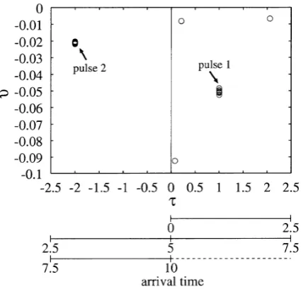
3.1 Two simple examples using complex Lorentzian We use synthesized complex frequency series consisting of a superposition of simple decaying sinusoids and white noise (Fig. 2(a)), which is equivalent to a superposition of the complex Lorentzian with noise in the time domain (Fig. 2(b)). The frequency series is synthesized for a frequency between 0 and 40 with interval 0.2, whose Nyquist travel time is 2.5. We apply the algorithm defined in the previous section to this synthetic data. The trial AR order ranges from 1 to 9, and the two-parameter AIC is calculated to determine the optimum number of wave elements for each AR order. Figure 3 plots the determined complex travel times of wave elements for all the trial AR orders in the similar way to the frequency-growth rate (f-g) diagram (Horiet al., 1989)
Fig. 2. (a) The transfer function in the frequency domain consisting of a superposition of two decaying sinusoids and Gaussian white noise. (b) The corresponding impulse response function obtained by the inverse Fourier transform of (a).
Fig. 3. Plots of the complex travel times for all the trial AR orders (1–9) estimated from the frequency series in Fig. 2(a). The relation between the real part of the complex travel time and arrival time due to the aliasing in the the time domain is also illustrated. The clusters of points represent clear signal, and scattered points represent incoherent noise.
in the Sompi method. The relation between the real part of complex travel time and arrival time due to the aliasing in the time domain is also illustrated in Fig. 3.
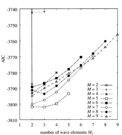
Compari-Fig. 4. Plots of the two-parameter AIC against the number of wave elements as a function of the AR order greater than 2.
Fig. 5. Comparison of the determined complex travel times and ampli-tudes with input values: (a) the real part of complex travel time, (b) the imaginary part of complex travel time, (c) the absolute value of complex amplitude, and (d) the phase of complex amplitude. Open circles are determined values plotted against the AR order. Solid and dotted lines represent input values of thefirst and the second pulses, respectively.
son of the determined complex travel times and amplitudes with input values is shown in Fig. 5, where we plot deter-mined values against the AR order. We can see a successful recovery of input signals for the AR orders larger than 2.
We also synthesized an impulse sequence consisting of the same two impulses as in Fig. 2, but much closer and hardly resolvable in time as shown in Figs. 6(a) and (b). Fig. 6(c) gives an expanded view of the two impulses. We use the bandpassfiltering and alias-folding technique to analyze this series with a box car time window of 1.25 ± 0.25. The determined complex travel times of wave elements are then plotted in Fig. 6(d) for all the trial AR orders (M = 1 ∼ 9), in which we find two densely populated regions very
Fig. 6. (a) The transfer function in the frequency domain consisting of a superposition of two decaying sinusoids, whose complex travel times are very close to each other, and Gaussian white noise. (b) The impulse response function obtained by the inverse Fourier transform of (a). (c) An enlargement of the pulse in (b), which consists of two closely spaced pulses (dashed and dotted lines). (d) Plots of complex travel times for all the trial AR orders (1–9) estimated for the frequency series in (b) with the bandpassfiltering and alias folding technique. Crosses in (d) indicate input values of the complex travel times. A cluster denoted by B at the window edge is spurious as originated from thefiltering.
close to input values. Thus, our method with the bandpass
filtering and alias-folding technique successfully resolved the two pulses. These are clearly distinguished by the difference of the real as well as imaginary part of complex travel times in Fig. 6(d).
3.2 Dispersive wave with physical dispersion
We synthesize a causal model of dispersive elastic wave with attenuation based on a theory of Azimiet al.(1968), in which the complex wavenumber is given by
Re[k˜(ω)]= ω c∞ +
2α0ω
π(1−α2 1ω2)
ln 1
α1ω
, (36)
I m[k˜(ω)]= α0ω 1+α1ω
(37)
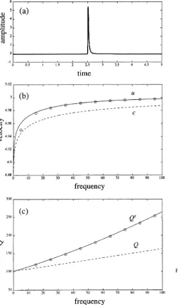
Fig. 7. A synthesized impulse response function (a), which shows asym-metric shape satisfying the causality. Estimated velocities (b) and quality factors (c) are indicated by circles with the theoretical curves for the group velocityuand the related quality factorQg(solid lines) and the phase velocitycand the related quality factorQ(dashed lines).
100 withx =12.5, we obtain the transfer function, whose inverse Fourier transform is shown in Fig. 7(a). The pulse shows an asymmetric shape satisfying causality: a sharp rise at the onset time with a trailing tail.
We use the noise-free frequency series of transfer function and the AR order corresponding to the number of input pulse to test whether our method with the band-limited analysis provides unbiased estimates of the complex travel times for the dispersive wave. We use a successive frequency band of 10 between 0 and 100. For the determined complex travel time in each frequency band, the velocity is calculated as the travel distance divided by the arrival time andQis calculated from
Q(ω0)= − τ(ω 0) 2υ(ω0)
. (38)
Fig. 8. (a) Estimated dimensionless velocities of the Rayleigh waves (cir-cles) with the theoretical dimensionless group velocity calculated by the Thomson-Haskell’s method (solid lines). See text for details. (b) Multi-filter analysis of the Rayleigh waves for the same waveform data as in (a). Gray scale indicates the common logarithm of the amplitude normalized by a maximum amplitude in each frequency band.
We plot the estimated velocities with the theoretical phase and group velocities in Fig. 7(b), and estimatedQwith the theoreticalQandQgin Fig. 7(c) against frequency. Except
for the lowest frequency band, in which theoretical velocity changes abruptly against frequency, the estimated velocity andQare in excellent agreement with the theoretical group velocity andQg.
3.3 Surface wave with structural dispersion
We apply our algorithm to structural dispersion analysis of a Rayleigh wave. As a simple example, we use a two-layer model for which the synthetic transfer function of the surface displacement in the radial direction due to a vertical point force on the surface is calculated using the reflectivity method (Koketsu, 1985). TheSwave velocities of the two layers are related byVS2=1.43VS1, while thePwave velocities are
0 and 2f0with an interval of 0.0008f0.
We apply the band-limited analysis to the transfer function for the whole frequency range. The synthetic transfer func-tion is divided into 64 segments. Each segment contains 64 data points and the width of the frequency band is 0.0512f0. The bandpassfiltering and alias folding technique is used to determine the arrival time of the Rayleigh wave in each fre-quency band. The velocity is calculated as the travel distance divided by the arrival time.
For comparison, we also analyze the same transfer func-tion using the multi-filter technique (Dziewonskiet al., 1969) commonly used for the dispersion analysis of surface waves. We apply the Gaussian frequency window to each of the successive frequency segments. The interval of the central frequency is 0.0512f0, which is the same as the band width used in the analysis of the AR modeling, and the width of Gaussian windows are proportional to the central frequen-cies. We convert each windowed frequency series into the time domain data by the inverse Fourier transform.
The results of the analysis of the AR modeling and the multi-filter analysis are shown in Fig. 8, respectively. In Fig. 8(a), we plot the dimensionless group velocities esti-mated for all the trial AR orders (1–10) in each frequency band with the theoretical dispersion curves up to the second higher modes calculated by means of the Thomson-Haskell method (Thomson, 1950; Haskell, 1953). Although there ex-ist scattered points for estimated wave elements originated from incoherent noise, densely populated regions are in good agreement with the theoretical curves up to the second higher modes. As shown in Fig. 8(b) of multi-filter analysis, the fundamental mode is identified with a clear peak in each fre-quency band. While we can recognize the branches of the higher modes in Fig. 8(b), their peaks are generally broad due to the operation of the Gaussian frequency window, indicat-ing difficulties in determining group velocities accurately, in contrast with our result.
4.
Discussions
We have presented a method to determine the complex travel times based on the AR modeling of a complex fre-quency series of transfer function. In the Sompi method, the AR equation is the same as Eq. (17) but the AR coefficients are real. A complex solution ofzfor real AR coefficients is always accompanied by its complex conjugate solution, and the number of independent solutions becomesM/2 for even M (an odd-order equation includes real roots forz). On the other hand, we have defined AR coefficients as the complex values for the complex series, resulting in M independent solutions ofzfor the Mth-order equation. In this sense we have presented a more general theory of a series analysis based on this AR equation.
Our basic assumption is that a complex frequency series consists of coherent simple decaying (or growing) oscilla-tions and incoherent noise, for which we can apply the com-plex AR equation to determine the comcom-plex travel times and amplitudes. Our AR model in the frequency domain corre-sponds to the complex Lorentzian in the time domain, which violates causality. Nonetheless, our AR model is justified for two reasons: (1) Theoretically, the impulse model violating causality is used only for narrow frequency bands, for which
causality constraint is meaningless: (2) In practice, our nu-merical test based on the dispersive wave satisfying causality show a reasonable and consistent result.
Another advantage of our method is that not only the ar-rival time but also the pulse width can be estimated from the complex travel time. The pulse width is related to anelas-tic structure of medium represented by the quality factor Q along the propagation ray path. Anelastic structure is poorly understood compared with elastic structure, although Q is an important parameter in understanding materials and their physical states within the earth. In previous studies, t∗ or differentialt∗(Teng, 1968) of thefirst arrival pulse has been used to investigateQstructure (e.g. Evans and Zucca, 1993). t∗is related to the imaginary part of travel timeυby
t∗= −2πυ. (39)
Least squaresfit to the slope of logarithmic Fourier spectrum of the seismogram has been commonly used for estimation oft∗. However, this method cannot resolve closely spaced pulses within a target time window (Evans and Zucca, 1988). Our method successfully resolved such pulses as demon-strated in Section 3.1, thus providing more accurate estimates of pulse widths and thereforeQstructures.
Another advantage of our method is its high resolvability of the complex travel time. The Sompi algorithm based on the AR modeling has theoretically infinite travel time res-olution, although limited by the presence of noise. On the other hand, the travel time resolution based on the Fourier method is limited by the length of frequency series as well as the tapering. As demonstrated in the dispersion analysis of surface waves in Section 3.3, the Fourier method requires a window with tapering in a narrow target frequency band to reduce side lobe interference by nearby peaks in the time domain. This phenomenon also reduces the resolution of the central peak while determining the arrival time. In the Sompi algorithm, however, based on the AR modeling of a frequency series, we can use the box-car window for a target frequency band without side lobe interference, enabling high resolution estimation of the arrival time.
Although our method has been developed for analysis of ACROSS data, this method can be widely applied to analysis of seismograms for active and passive sources after an appro-priate deconvolution of source effects. Our numerical tests demonstrate the applicability of our method with the high ac-curacy and resolvability. Although some practical problems such as error analysis are not treated in this paper, this method provides a new approach for event analysis, and a useful tool for the complex travel time analysis of seismograms.
Acknowledgments. Comments from Benjamin F. Chao and an anonymous reviewer help improved the manuscript.
References
Aki, K. and P. G. Richards,Quantitative seismology:Theory and methods, 932 pp., Freeman and Co., 1980.
Azimi, Sh. A., A. Y. Kalinin, V. B. Kalinin, and B. L. Pivovarov, Impulse and transient characteristics of media with linear and quadratic absorption laws,Izv. Earth Phys.,2, 88–93, 1968.
Chao, B. F. and F. Gilbert, Autoregressive estimation of complex eigen-frequencies in low frequency seismic spectra,Geophys. J. R. Astr. Soc., 63, 641–657, 1980.
Childers, D. G., D. P. Skinner, and R. C. Kemerait, The Cepstrum: A guide to processing,Proc. IEEE,65, 1428–1442, 1977.
Dziewonski, A., S. Bloch, and M. Landisman, A technique for analysis of transient seismic signals,Bull. Seism. Soc. Am.,59, 427–444, 1969. Evans, J. R. and J. J. Zucca, Active high-resolution seismic tomography
of compressional wave velocity and attenuation structure at Medicine Lake Volcano, northern California Cascade Range,J. Geophys. Res.,93, 15016–15036, 1988.
Evans, J. R. and J. J. Zucca, Active source, high-resolution (NeHT) tomog-raphy: velocity and Q, inSeismic Tomography, edited by H. M. Iyer and K. Hirahara, Chap. 25, pp. 695–732, Chapman and Hall, 1993. Haskell, N. A., The dispersion of surface waves in multilayered media,Bull.
Seism. Soc. Am.,43, 17–34, 1953.
Hildebrand, F. B.,Introduction to Numerical Analysis, Chap. 9, 511 pp., New York: McGraw-Hill, 1956.
Hori, S., Y. Fukao, M. Kumazawa, M. Furumoto, and A. Yamamoto, A new method of spectral analysis and its application to the Earth’s free oscillations: The“Sompi”method,J. Geophys. Res.,94(B6), 7535–7553, 1989.
Kay, S. M. and S. L. Marple, Spectrum analysis—a modern perspective,
Proc. IEEE,69, 1380–1419, 1981.
Koketsu, K., The extended reflectivity method for synthetic near-field seis-mograms,J. Phys. Earth,33, 121–131, 1985.
Kumazawa, M. and Y. Takei, Active method of monitoring underground structures by means of accurately controlled rotary seismic sources. 3.
Event detection from a small number of Fourier components observed by ACROSS system,Abstr. Seism. Soc. Jpn.,2, 160, 1994 (in Japanese). Kumazawa, M., Y. Imanishi, Y. Fukao, M. Furumoto, and A. Yamamoto, A
theory of spectral analysis based on the characteristic property of a linear dynamic system,Geophys. J. Int.,101, 613–630, 1990.
Matsuura, T., Y. Imanishi, M. Imanari, and M. Kumazawa, Application of a new method of high-resolution spectral analysis,“Sompi,”for free induction decay of nuclear magnetic resonance,Appl. Spectrosc., 44, 618–626, 1990.
Oppenheim, A. V. and D. W. Schafer,Digital signal processing, pp. 480– 531, Prentice-Hall International, London, 1975.
Pisarenko, V. F., On the estimation of spectra by means of nonlinear func-tions of covariance matrix,Geophys. J. R. Astr. Soc.,28, 511–531, 1972. Price, H. J., An improved Prony algorithm for exponential analysis, in Pro-ceedings of the IEEE International Symposium on Electro-magnetic Com-patibility, pp. 310–313, Institute of Electrical and Electronics Engineers, New York, 1979.
Shankland, T. J., P. A. Johnson, and T. M. Hopson, Elastic wave attenua-tion and velocity of Berea sandstone measured in the frequency domain,
Geophys. Res. Lett.,20(5), 391–394, 1993.
Teng, T.-L., Attenuation of body waves and theQstructure of the mantle,
J. Geophys. Res.,73, 2195–2208, 1968.
Thomson, W. T., Transmission of elastic waves through a stratified solid,J. Appl. Phys.,21, 89–93, 1950.