A modified algorithm for computation issues in UAV enabled wireless communications

(1)

R E S E A R C H

Open Access

A modified algorithm for computation

issues in UAV-enabled wireless

communications

Bing Hu

1

, Xiaojian Ding

2

, Fan Yang

2

and Jian Liu

2*

Abstract

Unmanned aerial vehicles (UAVs) in wireless communication have received significant interests recently due to its low cost and flexibility in providing wireless connectivity in areas without infrastructure coverage. In this paper, we optimize the location of UAVs to maximize their coverage areas. We propose a modified artificial bee colony (MABC) incorporating bee number reallocation and a new search equation. In the proposed algorithm, a greater number of bees in the population are assigned to execute local searches near food sources to enhance solution accuracy, and the bees are guided by elite vectors to enable the algorithm to rapidly converge to a potentially globally optimal position. The deployment of UAVs is thus obtained. The experimental results show that the proposed algorithm achieves great improvements over the traditional algorithm.

Keywords: Unmanned aerial vehicles, Mobile base station, Artificial bee colony, Parameter estimation

1 Introduction

Unmanned aerial vehicles (UAVs) have attracted

widespread attention over the past decade [1–3], involv-ing applications such as surveillance [4, 5], aerospace imaging [6,7], and cargo transportation [8,9]. Extensive research is also devoted to the use of drones as different types of wireless communication platforms, such as aero-nautical mobile base stations (BS) [10–12], mobile relays [13], and flight cloud computing [14]. In particular, the use of UAVs as airborne BSs is envisioned as a promising solution to enhance the performance of existing cellular systems [15].

In a UAV-assisted network, UAVs are deployed to pro-vide wireless connectivity to ground users. In practice, UAVs can move freely in three-dimensional space for bet-ter performance. Due to the high mobility of drones, the deployment of drone-assisted communication sys-tems is faster and more flexible, making them particularly suitable for on-demand applications or accidents. Fur-thermore, the UAV-ground link is more likely to have a line-of-sight (LoS) channel than the ground-to-ground

*Correspondence:[email protected]

2_{College of Information Engineering, Nanjing University of Finances and} Economics, 210023 Nanjing, China

Full list of author information is available at the end of the article

link in the terrestrial system [16–19], thus providing a higher link capacity. In addition, UAV-assisted commu-nication provides additional design freedom for perfor-mance improvements by dynamically optimizing the UAV position to best meet communication requirements. In this paper, we have studied a general-purpose multi-UAV wireless communication system in which multiple drones are used to serve a group of users on the ground within a given group of users.

Research on wireless networks supporting static drones has focused on drone deployment/layout optimization, which acts as a quasi-static BS in the air to support ter-restrial users in specific areas [20]. In such a scene, the deployment of UAVs is an important and fundamental issue. The artificial bee colony (ABC) evolutionary algo-rithm is known to be powerful, effective, and competitive in the above problem. However, its success is hindered by its slow convergence speed and poor local search capa-bility [21–23]. In this paper, we reallocate the number of employed and onlooker bees to generate a better bal-ance between global and local search. The proportion of employed bees is decreased while that of onlooker bees is increased in the colony. In addition, a new search equation to accelerate the algorithm’s convergence speed is also proposed. The one-dimensional search strategy, which

(2)

(3)

typically guarantees a global search [24], is retained in this paper. Finally, a series of benchmark functions are employed to test the proposed algorithm’s effectiveness on both theoretical and applied problems.

The remainder of this paper is organized as follows: Section2describes traditional artificial bee colonies, and Section3presents a detailed description of the proposed modified ABC algorithm. In Section4, benchmarks and parameter estimation problem are presented, and a suite of experiments is conducted. Section 5 concludes the paper.

2 Method

Firstly proposed by Karaboga in 2005, an artificial bee colony simulates the foraging behavior of bees in a colony. In the algorithm, three types of bees cooperatively work with each other: employed bees are distributed to enable the exploration of a food source’s position within the entire search space, onlooker bees are assigned to enable exploitation near the neighbor areas of food sources, and scouts are designed to help the algorithm avoid local optima.

In the traditional artificial bee colony algorithm, the entire population is divided into employed bees and onlooker bees. Thus, the number of employed bees and onlooker bees are equivalent to both each other and the number of food sources. To illustrate each part of

ABC algorithm in greater detail, we describe them in succession.

2.1 Initialization

For a given optimization problem, letlandudenote the lower and upper border of the parameters. LetNPdenote the population size, and letDdenote the dimension of the problem. Each food source can be initialized as

Fij=lij+rand

uij−lij

(1)

whereirepresents theith food source, andjdenotes the

jth dimension,i=1, 2, ...,NP/2 ,j=1, 2, ...,D. 2.2 Employed bees

At each iteration, the employed bees search the entire space. Thus, they are responsible for conducting a global search. Each food source corresponds to an employed bee. The search equation is

trialij=Fij+rand(−1, 1)

Frj−Fij

(2)

whereFris a neighbor of food sourceFi, andris selected

within the range of [1,NP/2],r=i.

In the traditional ABC algorithm, each newly generated position is stored in a trial vector only if it improves upon the current food source’s position, and the

(4)

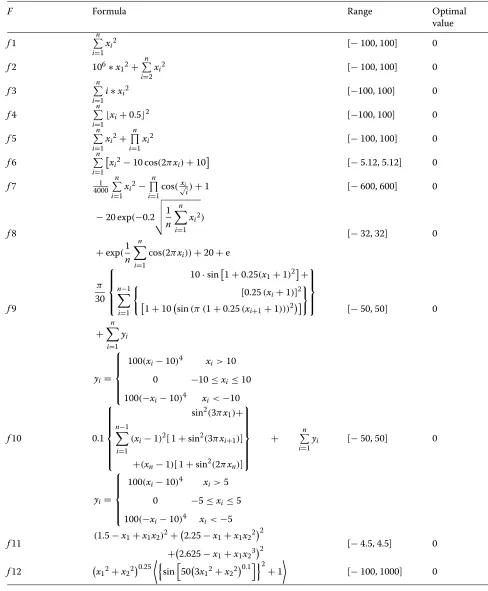
Table 1Detailed information on the 12 benchmarks

F Formula Range Optimal

(5)

Table 2Corresponding experimental settings

Dimension Maximum iteration number Maximum function evaluation number

(NP * maximum iteration number)

2 100 4000

10 1000 40,000

30 3000 120,000

50 5000 200,000

ing food source is updated, resulting in a so-called greedy search.

The objective value,fi, and fitness value,Fi, are

calcu-lated for each food source,i. For minimum optimization problems, the objective value is calculated by the

prob-lem’s mathematical expression, and the fitness value is calculated as

Fi=

1/(1+fi) if fi≥0

1+abs(fi) if fi<0 (3)

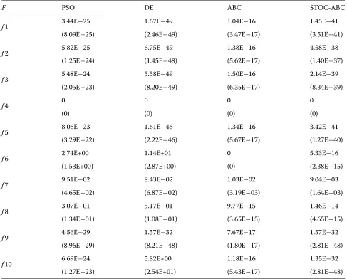
Table 3Comparison results (1),D= 10

F PSO DE ABC STOC-ABC

f1 3.44E−25 1.67E−49 1.04E−16 1.45E−41

(8.09E−25) (2.46E−49) (3.47E−17) (3.51E−41)

f2 5.82E−25 6.75E−49 1.38E−16 4.58E−38

(1.25E−24) (1.45E−48) (5.62E−17) (1.40E−37)

f3 5.48E−24 5.58E−49 1.50E−16 2.14E−39

(2.05E−23) (8.20E−49) (6.35E−17) (8.34E−39)

f4 0 0 0 0

(0) (0) (0) (0)

f5 8.06E−23 1.61E−46 1.34E−16 3.42E−41

(3.29E−22) (2.22E−46) (5.67E−17) (1.27E−40)

f6 2.74E+00 1.14E+01 0 5.33E−16

(1.53E+00) (2.87E+00) (0) (2.38E−15)

f7 9.51E−02 8.43E−02 1.03E−02 9.04E−03

(4.65E−02) (6.87E−02) (3.19E−03) (1.64E−03)

f8 3.07E−01 5.17E−01 9.77E−15 1.46E−14

(1.34E−01) (1.08E−01) (3.65E−15) (4.65E−15)

f9 4.56E−29 1.57E−32 7.67E−17 1.57E−32

(8.96E−29) (8.21E−48) (1.80E−17) (2.81E−48)

f10 6.69E−24 5.82E+00 1.18E−16 1.35E−32

(6)

F dABC distABC NSABC MABC

f1 3.59E−52 4.12E−76 3.80E−80 1.38E−149

(6.72E−52) (1.19E−75) (1.13E−79) (6.14E−149)

f2 7.34E−48 2.46E−74 9.29E−78 2.08E−147

(3.08E−47) (7.98E−74) (3.23E−77) (9.27E−147)

f3 3.96E−50 2.47E−76 1.68E−79 5.83E−146

(9.25E−50) (5.11E−76) (7.17E−79) (2.58E−145)

f4 0 0 0 0

(0) (0) (0) (0)

f5 9.29E−51 8.43E−75 3.13E−80 4.88E−112

(3.32E−50) (3.45E−74) (8.33E−80) (2.18E−111)

f6 0 0 0 0

(0) (0) (0) (0)

f7 1.01E−02 9.79E−03 1.07E−02 9.70E−03

(2.64E−03) (2.03E−03) (4.08E−03) (2.74E−03)

f8 9.95E−15 6.04E−15 4.44E−15 5.68E−15

(2.93E−15) (7.94E−16) (1.82E−15) (1.30E−15)

f9 1.57E−32 1.57E−32 7.59E−17 1.57E−32

(2.81E−48) (2.81E−48) (1.61E−17) (2.81E−48)

f10 1.35E−32 1.35E−32 1.35E−32 1.35E−32

(2.81E−48) (2.81E−48) (2.81E−48) (2.81E−48)

2.3 Onlooker bees

After the employed bees’ searches are completed, the onlooker bees initiate local searches around the food sources’ neighboring areas. In this phase, the onlookers select food sources by roulette wheel selection to enable exploitation. The search equation is identical to that of the employed bees presented in Eq. (2).

2.4 Scouts

When a food source cannot be improved upon for a cer-tain number of iterations, the corresponding employed bee turns into a scout and reinitializes the corresponding food source in the search space.

3 Modified Artificial Bee Colony (MABC)

The artificial bee colony algorithm is known for its strong global search and poor local search capabilities; thus, we

aim to compensate for this insufficiency on the basis of guaranteeing an advantage. With this purpose in mind, two modifications are proposed.

(7)

f1 2.05E−17 1.88E−47 8.13E−16 4.93E−40

(5.06E−17) (4.89E−47) (1.34E−16) (6.07E−40)

f2 5.15E−17 8.01E−48 8.98E−16 3.29E−38

(1.64E−16) (8.40E−48) (2.56E−16) (1.30E−37)

f3 1.81E−16 8.23E−47 8.69E−16 1.10E−38

(2.49E−16) (1.27E−46) (1.61E−16) (2.68E−38)

f4 0 0 0 0

(0) (0) (0) (0)

f5 1.82E+02 1.46E−41 8.77E−16 1.13E−39

(7.95E+02) (6.23E−41) (1.78E−16) (1.58E−39)

f6 2.94E+01 1.16E+02 6.17E−14 2.74E−14

(8.98E+00) (2.91E+01) (1.49E−13) (4.54E−14)

f7 1 1 1 1

(3.41E−16) (2.22E−16) (3.46E−16) (3.39E−16)

f8 7.72E−01 9.71E−01 1.20E−13 3.39E−13

(7.62E−02) (1.80E−01) (7.24E−14) (4.87E−13)

f9 3.11E−02 1.58E−32 7.75E−16 5.80E−31

(5.77E−02) (2.81E−34) (1.56E−16) (2.50E−30)

f10 2.85E+02 9.59E+01 8.54E−16 5.29E−32

(1.80E+02) (1.07E+02) (1.50E−16) (5.45E−32)

is equivalent to the number of employed bees, and each food source corresponds to one employed bee and three onlooker bees.

In the second modification, the search equation is changed. In a traditional artificial bee colony, an employed bee hunts for a food position depending on its memory of its previous position and a randomly selected neighboring food source; this hunting is blind and ineffective for local searches [24]. Considering this drawback, we propose a novel search equation to achieve a better balance between exploration and exploitation. Its mathematical expression is presented in Eq. (4).

trialij=Frj+rand(−1, 1)

Gj−Fij

(4)

whereFris a neighbor of food sourceFi, which is selected

in the same manner as that in Eq. (2).Gis the current best food source’s position. By introducing a best vector, bees can fly to the potential global point more rapidly.

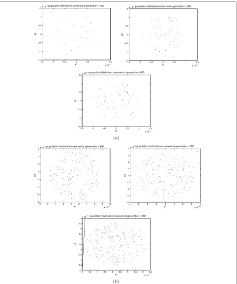
To demonstrate the effectiveness of Eq. (4), we con-duct experiments on the sphere function (f1) presented in Section 4. In this experiment, the population size is set to 100. Because we are demonstrating the search equation’s effectiveness, the comparison algorithms both adopt employed and onlooker bees as representing half of the colony. In this demonstration, we analyze the per-formance of the proposed Eq. (4) and traditional Eq. (2). Thus, the test dimension is selected to be 2 to allow for plotting the population distribution figures of different iterations. Figure1shows the results of the comparison.

(8)

f1 2.11E−49 1.24E−71 2.82E−70 3.01E−95

(5.00E−49) (3.21E−71) (6.64E−70) (1.24E−94)

f2 8.09E−47 1.22E−69 4.92E−69 1.42E−63

(1.45E−46) (2.65E−69) (1.81E−68) (6.35E−63)

f3 1.05E−47 2.91E−70 3.14E−67 6.68E−141

(1.90E−47) (5.43E−70) (1.35E−66) (2.99E−140)

f4 0 0 0 0

(0) (0) (0) (0)

f5 1.74E−48 2.22E−70 2.52E−70 5.77E−70

(3.70E−48) (3.92E−70) (7.51E−70) (2.58E−69)

f6 2.25E−14 0 1.78E−16 0

(7.36E−14) (0) (7.94E−16) (0)

f7 1 1 1 1

(3.89E−16) (4.88E−16) (4.82E−16) (4.87E−16)

f8 9.36E−14 4.48E−14 3.61E−03 3.53E−14

(4.43E−14) (5.79E−15) (1.61E−02) (4.09E−15)

f9 1.66E−32 1.57E−32 4.93E−16 1.57E−32

(1.88E−33) (2.81E−48) (1.34E−16) (2.81E−48)

f10 1.72E−32 1.35E−32 1.47E−29 1.35E−32

(8.10E−33) (2.81E−48) (2.19E−29) (2.81E−48)

and 800th generations, respectively. These experiments demonstrate that the proposed search equation might help bees converge to potentially global optima much more rapidly.

To further demonstrate the two modifications’ effective-ness, Section4evaluates MABC’s optimization accuracy on a series of benchmark experiments.

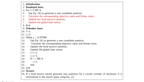
To illustrate the proposed MABC algorithm much more specifically, Fig.2gives its pseudo-code.

4 Simulation results and discussions

In this subsection, integral and comprehensive exper-iments are conducted to test MABC’s effectiveness. Section 4.1 gives detailed information on the twelve benchmarks of performance estimation criteria, and Section 4.2 presents the results of the comparison experiments using the proposed MABC and other

state-of-the-art algorithms. In Section 4.3, sub-experiments demonstrate each MABC modification’s effectiveness, and Section4.4describes a parameter estimation problem for frequency-modulated sound waves and discusses the MABC’s application performance.

4.1 Detailed benchmark information

(9)

f1 4.01E−13 1.82E−48 2.02E−15 1.10E−38

(4.99E−13) (3.67E−48) (4.37E−16) (3.59E−38)

f2 6.11E−13 1.51E−48 3.85E−15 2.17E−37

(6.85E−13) (1.99E−48) (2.58E−15) (6.74E−37)

f3 7.23E−12 3.53E−47 2.02E−15 5.36E−38

(1.41E−11) (4.84E−47) (7.81E−16) (9.72E−38)

f4 5.00E−02 0 5.00E−02 1.50E−01

(2.18E−01) (0) (2.24E−01) (3.66E−01)

f5 5.24E+04 1.03E−44 1.93E−15 4.12E−39

(8.21E+04) (2.78E−44) (4.77E−16) (4.52E−39)

f6 7.29E+01 1.63E+02 9.86E−12 1.31E−12

(1.56E+01) (4.88E+01) (2.12E−11) (2.73E−12)

f7 1 1 1 1

(1.76E−14) (1.99E−16) (8.35E−16) (5.04E−16)

f8 1.13E+00 8.18E−01 1.14E−12 2.76E−12

(1.62E−01) (2.51E−01) (2.87E−12) (6.70E−12)

f9 1.99E−01 5.18E−03 1.90E−15 5.69E−32

(6.76E−01) (2.26E−02) (5.33E−16) (2.57E−32)

f10 1.37E+03 7.88E+02 2.11E−15 9.42E−31

(4.01E+02) (2.87E+02) (6.27E−16) (1.57E−30)

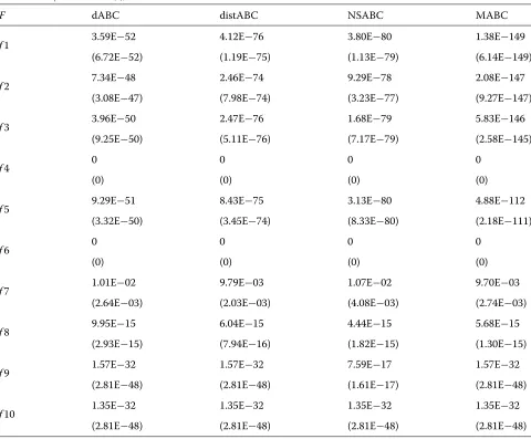
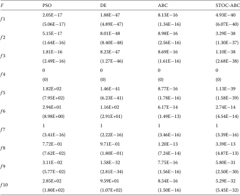
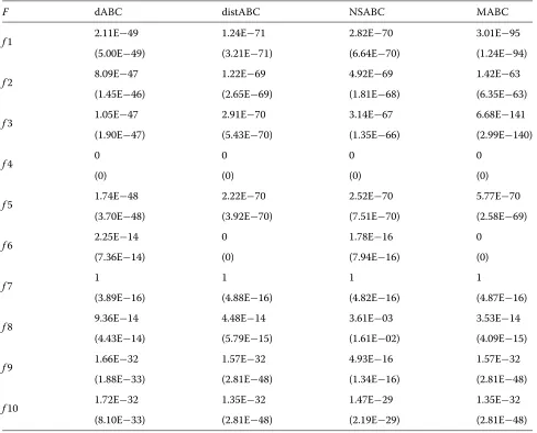
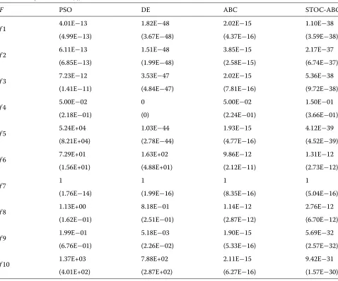
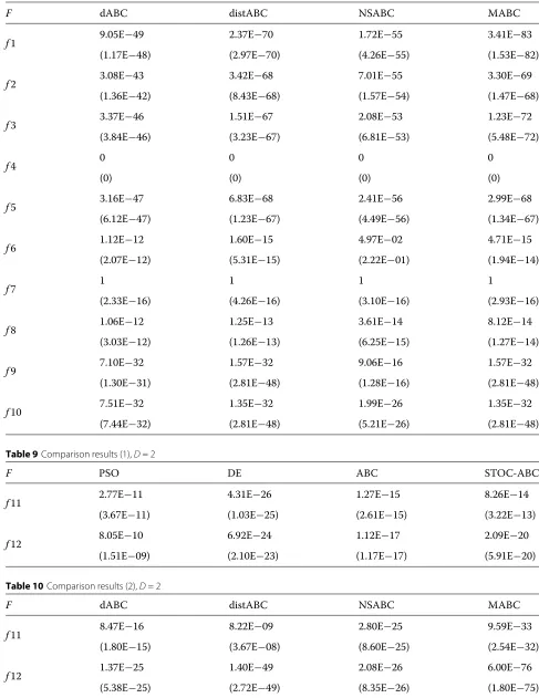
4.2 Comparison experiments

This subsection describes the comparison experiments conducted to demonstrate the proposed MABC’s effec-tiveness and competieffec-tiveness against other evolution-ary algorithms. In this phase, the selected comparison algorithms include traditional particle swarm optimiza-tion (PSO), differential evoluoptimiza-tion (DE), and artificial bee colony (ABC), as well as four ABC variants, includ-ing STOC-ABC [21], dABC [22], distABC [23], and NSABC [24].

In the experiments, the population size is set to 40. For the first ten benchmarks presented in Table1, all the algorithms are tested on 10, 30, and 50 dimensions. For the last two benchmarks, the comparison algorithms are tested on two dimensions. The corresponding maximum iteration and function evaluation numbers are presented in Table 2. For the sake of fairness, all the trials are repeated 50 times, and the corresponding mean fitness

values (first row) and standard deviations (second row) are recorded, as presented in Tables 3, 4, 5, 6, 7, 8, 9, and10.

(10)

f1 9.05E−49 2.37E−70 1.72E−55 3.41E−83

(1.17E−48) (2.97E−70) (4.26E−55) (1.53E−82)

f2 3.08E−43 3.42E−68 7.01E−55 3.30E−69

(1.36E−42) (8.43E−68) (1.57E−54) (1.47E−68)

f3 3.37E−46 1.51E−67 2.08E−53 1.23E−72

(3.84E−46) (3.23E−67) (6.81E−53) (5.48E−72)

f4 0 0 0 0

(0) (0) (0) (0)

f5 3.16E−47 6.83E−68 2.41E−56 2.99E−68

(6.12E−47) (1.23E−67) (4.49E−56) (1.34E−67)

f6 1.12E−12 1.60E−15 4.97E−02 4.71E−15

(2.07E−12) (5.31E−15) (2.22E−01) (1.94E−14)

f7 1 1 1 1

(2.33E−16) (4.26E−16) (3.10E−16) (2.93E−16)

f8 1.06E−12 1.25E−13 3.61E−14 8.12E−14

(3.03E−12) (1.26E−13) (6.25E−15) (1.27E−14)

f9 7.10E−32 1.57E−32 9.06E−16 1.57E−32

(1.30E−31) (2.81E−48) (1.28E−16) (2.81E−48)

f10 7.51E−32 1.35E−32 1.99E−26 1.35E−32

(7.44E−32) (2.81E−48) (5.21E−26) (2.81E−48)

f11 2.77E−11 4.31E−26 1.27E−15 8.26E−14

(3.67E−11) (1.03E−25) (2.61E−15) (3.22E−13)

f12 8.05E−10 6.92E−24 1.12E−17 2.09E−20

(1.51E−09) (2.10E−23) (1.17E−17) (5.91E−20)

f11 8.47E−16 8.22E−09 2.80E−25 9.59E−33

(1.80E−15) (3.67E−08) (8.60E−25) (2.54E−32)

f12 1.37E−25 1.40E−49 2.08E−26 6.00E−76

(11)

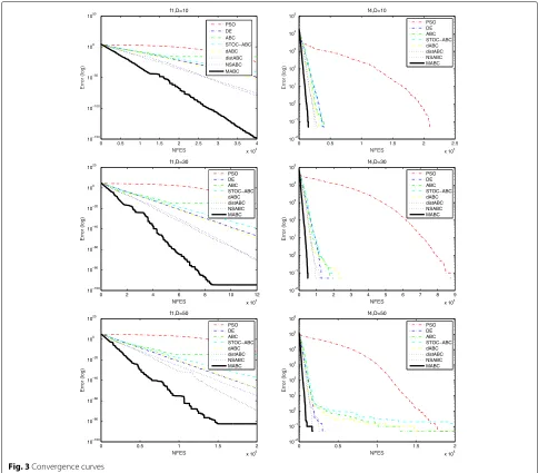
Fig. 3Convergence curves

bees does not cripple their exploration ability, and increasing the number of onlooker bees improves their exploitation capability. In addition, the proposed MABC algorithm’s successful performance on low dimensional functions demonstrates that it is unlimited by a problem’s dimension. For the unimodal functions, with the excep-tion of the soluexcep-tion accuracy presented in the results table, convergence speed is another important evaluation crite-rion. Thus, we plot the convergence curves off1 andf4 in Fig.3.f1 is the sphere function, which is also the most representative unimodal function, andf4 is the unimodal function for which most of the algorithms obtain global optima. Thus, convergence speed functions as the main evaluation criterion for the evolution algorithms’ performance.

4.3 Effectiveness of the two modifications

Whereas the previous subsection presented an integral demonstration of MABC’s performance, the present sub-section covers the experiments to test the effectiveness of each MABC modification, which are conducted in two groups.

(12)

Fig. 4Demonstration of the first modification’s effectiveness

(13)

Table 11Comparison results for ABC, ABC1, ABC2, and MABC

ABC ABC1 ABC2 MABC

f1 1.04E−16 3.08E−92 1.77E−73 1.38E−149

(3.47E−17) (1.27E−91) (3.31E−73) (6.14E−149)

f2 1.45E−16 3.45E−91 2.44E−69 5.97E−138

(6.96E−17) (1.29E−90) (6.70E−69) (2.67E−137)

f3 1.30E−16 9.24E−92 1.62E−71 1.05E−148

(6.02E−17) (3.41E−91) (3.13E−71) (4.11E−148)

f4 0 0 0 0

(0) (0) (0) (0)

f5 1.20E−16 1.98E−93 1.21E−71 7.91E−144

(5.58E−17) (7.88E−93) (2.99E−71) (2.13E−143)

f6 0 0 0 0

(0) (0) (0) (0)

f7 1.07E−02 1.12E−02 8.63E−03 9.62E−03

(3.96E−03) (4.47E−03) (9.24E−04) (2.08E−03)

f8 2.27E−13 1.12E−14 7.11E−15 5.86E−15

(9.66E−13) (4.06E−15) (1.95E−15) (1.09E−15)

f9 1.01E−16 1.57E−32 1.57E−32 1.57E−32

(4.37E−17) (2.81E−48) (2.81E−48) (2.81E−48)

f10 1.30E−16 1.35E−32 1.35E−32 1.35E−32

(4.78E−17) (2.81E−48) (2.81E−48) (2.81E−48)

2) New search equation

The second group of experiments tests the proposed search equation’s competitiveness. Thus, we design ABC2, whose search equation adopts Eq. (4). The remaining parts of the algorithm remain consistent with the traditional ABC algorithm.

In this subsection, the test dimension is set to 10, and the other settings are identical to those in Section4.4. Figures4and5show the comparison results for the two experimental groups on several representative benchmarks. The figures show that each modification greatly improves upon the traditional ABC. The

Table 12Experimental results on parameter estimation for frequency-modulated sound waves

PSO DE ABC STOC-ABC

Mean 29.9601 29.9601 27.7173 46.2575

SD 0.2161 0.2161 3.7348 20.9301

dABC distABC NSABC MABC

Mean 27.8124 26.0923 36.3419 25.5948

(14)

detailed accuracy and standard deviation data for the first ten benchmarks are presented in Table11, which also demonstrates each modification of MABC’s effectiveness.

4.4 Parameter estimation problem for frequency-modulated sound waves

The synthesis of frequency-modulated sound waves [28] plays a significant role in modern music systems [29–32]. In this process, parameter estimation consists of a six-dimensional optimization problem. The goal is to generate a sound,A, that is very similar to a certain sound,B. Let

X= {x1,x2,x3,x4,x5,x6} represent the six parameters to be optimized. The mathematical expressions of soundA

wave can then be formulated as follows:

wavesA(t)=x1sin

The objective function of this problem is the summation of the squared errors between sound wavesAandB, as presented in Eq. (6):

This is a minimization problem with complex local optima. For all six parameters, the lower bound is - 6.4, and the maximum bound is 6.35. In our experiment, the population size is set to 40, and the maximum function evaluation number is set to 30,000. When the maximum function evaluation number is satisfied, the correspond-ing trial terminates. The experimental results for the eight algorithms employed in Section 4.4are presented in Table 12, which demonstrate the proposed MABC algorithm’s competitiveness on a real-world application problem.

5 Conclusion

In this paper, we studied the problem about the placement of UAVs in UAV-aided wireless communications. We first exploit the controllable channel variation induced by dif-ferent locations of base stations, the coverage areas of UAVs are maximized via optimizing their locations. Then, we formulate the original problem and try to solve it by artificial bee colony algorithm. Instead of using traditional algorithms, we propose a modified artificial bee colony. By reallocating the number of employed and onlooker bees

and improving the search equation, convergence speed and enhancing local search capability are both acceler-ated. Furthermore, it generates a better balance between global and local search. Experimental results show that the new approach of placement problem improves the performance of UAV communication systems.

Abbreviations

ABC: Artificial bee colony; BS: Base station; LoS: Line-of-sight; UAV: Unmanned aerial vehicle

Acknowledgments Not applicable

Authors’ contributions

BH is the main author of the current paper. BH contributed to the development of the ideas, design of the study, theory, result analysis, and article writing. XD carried out the experimental work and the data collection and interpretation. FY finished the analysis and interpretation of data and drafted the manuscript. JL conceived and designed the experiments, and undertook revision works of the paper. All authors read and approved the final manuscript.

Funding

This work was supported by the National Natural Science Foundation of China (Grant No. 61802200), the Natural Science Foundation of Jiangsu (grant nos. BK20160148, BK20180745, and BK20190789) and the Natural Science Foundation of the Jiangsu Higher Education Institutions of China (grant nos. 18KJB520035, 19KJB520035, and 19KJB130006). The authors would like to thank those who have provided helpful suggestions.

Availability of data and materials

Data sharing is not applicable to this article as no datasets were generated or analyzed during the current study.

Competing interests

The authors declare that they have no competing interests.

Author details

1_{College of Modern Posts, Nanjing University of Posts and}

Telecommunications, 210003 Nanjing, China.2_{College of Information}

Engineering, Nanjing University of Finances and Economics, 210023 Nanjing, China.

Received: 17 August 2019 Accepted: 31 October 2019

References

1. Y. Zeng, R. Zhang, T. J. Lim, Wireless communications with unmanned aerial vehicles: opportunities and challenges. IEEE Commun. Mag.54(5), 36–42 (2016)

2. F. Cheng, G. Guan, N. Zhao, F. R. Yu, Y. Chen, J. Tang, H. Sari, inProc. ICNC’18. Caching UAV assisted secure transmission in small-cell networks, (2018), pp. 1–6.https://doi.org/10.1109/iccnc.2018.8390316

3. C. Li, H. J. Yang, F. Sun, J. M. Cioffi, L. Yang, Adaptive overhearing in two-way multi-antenna relay channels. IEEE Signal Process. Lett.23(1), 117–120 (2016)

4. H. Zhang, C. Jiang, J. Cheng, V. C. M. Leung, Cooperative interference mitigation and handover management for heterogeneous cloud small cell networks. IEEE Wirel. Commun.22(3), 92–99 (2015)

5. Y. Zeng, R. Zhang, Energy-efficient UAV communication with trajectory optimization. IEEE Trans. Wirel. Commun.16(6), 3747–3760 (2017) 6. C. Li, H. J. Yang, F. Sun, J. M. Cioffi, L. Yang, Multiuser overhearing for

cooperative two-way multiantenna relays. IEEE Trans. Veh. Technol.65(5), 3796–3802 (2016)

(15)

8. F. Jiang, A. L. Swindlehurst, Optimization of UAV heading for the ground-to-air uplink. IEEE J. Sel. Areas Commun.30(5), 993–1005 (2012) 9. H. Wang, G. Ding, F. Gao, J. Chen, J. Wang, L. Wang, Power control in

UAV-supported ultra dense networks: communications, caching, and energy transfer. IEEE Commun. Mag. (2018). to appear.https://doi.org/10. 1109/mcom.2018.1700431

10. C. Jie, Z. Bu, Y. Wang, H. Yang, J. Jiang, H. Li, Detecting prosumer-community group in smart grids from the multiagent perspective. IEEE Trans. Syst. Man Cybern. Syst.49(8), 1652–1664 (2019) 11. J. Lyu, Y. Zeng, R. Zhang, T. J. Lim, Placement optimization of

UAV-mounted mobile base stations. IEEE Commun. Lett.21(3), 604–607 (2017)

12. Z. Bu, J. Li, C. Zhang, J. Cao, A. Li, Y. Shi, Graph K-means based on leader identification, dyname game, and opinion dynamics. IEEE Trans. Knowl. Data Eng.https://doi.org/10.1109/TKDE.2019.2903712

13. M. Mozaffari, W. Saad, M. Bennis, M. Debbah, Efficient deployment of multiple unmanned aerial vehicles for optimal wireless coverage. IEEE Commun. Lett.20(8), 1647–1650 (2016)

14. C. Li, F. Sun, J. M. Cioffi, L. Yang, Energy efficient MIMO relay transmissions via joint power allocations. IEEE Trans. Circ. Syst.61(7), 531–535 (2014) 15. J. Liu, Y. Gu, L. Zha, Y. Liu, J. Cao, Event-triggered H-infinity load frequency

control for multi-area power systems under hybrid cyber attacks. IEEE Trans. Syst. Man Cybern. Syst.49(8), 1665–1678 (2019)

16. W. Wu, B. Wang, Y. Zeng, H. Zhang, Z. Yang, Z. Deng. Robust secure beamforming for wireless powered full-duplex systems with self-energy recycling, (2017). to be published in.https://doi.org/10.1109/tvt.2017. 2744982

17. J. Liu, M. Yang, E. Tian, J. Cao, S. Fei, Event-based security controller design for state-dependent uncertain systems under hybrid-attacks and its application to electronic circuits. IEEE Trans. Circ. Syst. I Regular Pap. https://doi.org/https://doi.org/10.1109/TCSI.2019.2930572

18. C. Li, S. Zhang, P. Liu, F. Sun, J. M. Cioffi, L. Yang, Overhearing protocol design exploiting inter-cell interference in cooperative green networks. IEEE Trans. Veh. Technol.65(1), 441–446 (2016)

19. W. Wu, N. Wang, Efficient transmission solutions for MIMO wiretap channels with SWIPT. IEEE Commun. Lett.19(9), 1548–1551 (2015) 20. C. Li, P. Liu, C. Zou, F. Sun, J. M. Cioffi, L. Yang, Spectral-efficient cellular

communications with coexistent one- and two-hop transmissions. IEEE Trans, Veh. Technol.65(8), 6765–6772 (2016)

21. M. S. Kiran, H. Hakli, M. Gunduz, et al., Artificial bee colony algorithm with variable search strategy for continuous optimization. Inform. Sci.300, 140–157 (2015)

22. X. Li, G. Yang, Artificial bee colony algorithm with memory. App. Soft. Comput.41, 362–372 (2016)

23. Y. Shi, C. M. Pun, H. Hu, et al., An improved artificial bee colony and its application. Knowl. Syst.107, 14–31 (2016)

24. K. Binder, D. Heermann, L. Roelofs, et al., Monte carlo simulation in statistical physics. Comput. Phys.7(2), 156–157 (1993)

25. R. H. Swendsen, J. S. Wang, Nonuniversal critical dynamics in monte carlo simulations. Phys. Rev. Lett.58(2), 86 (1987)

26. P. P. Boyle, Options: a monte carlo approach. J. Finan. Econ.4(3), 323–338 (1977)

27. X. Yao, Y. Liu, G. Lin, Evolutionary programming made faster. IEEE Trans. Evol. Comput.3(2), 82–102 (1999)

28. M. M. Ali, C. Khompatraporn, Z. B. Zabinsky, A numerical evaluation of several stochastic algorithms on selected continuous global optimization test problems. J. Global. Optim.31(4), 635–672 (2005)

29. H. Gao, S. Kwong, J. Yang, et al., Particle swarm optimization based on intermediate disturbance strategy algorithm and its application in multi-threshold image segmentation. Inform. Sci.250, 82–112 (2013) 30. P. Wu, Y. Han, T. Chen, et al., Causal inference for Mann-Whitney-Wilcoxon

rank sum and other nonparametric statistics. Stat. Med.33(8), 1261–1271 (2014)

31. L. De Capitani, D. De Martini, Reproducibility probability estimation and testing for the Wilcoxon rank-sum test. J. Stat. Comput. Simul.85(3), 468–493 (2015)

32. R. C. Blair, J. J. Higgins, A comparison of the power of Wilcoxon’s rank-sum statistic to that of Student’s t statistic under various nonnormal

distributions. J. Educ. Behav. Stat.5(4), 309–335 (1980)

Publisher’s Note