R E S E A R C H
Open Access
User grouping and resource allocation
in multiuser MIMO systems under SWIPT
Javier Rubio and Antonio Pascual-Iserte
*Abstract
This paper considers a broadcast multiple-input multiple-output (MIMO) network with multiple users and
simultaneous wireless information and power transfer (SWIPT). In this scenario, it is assumed that some users are able to harvest power from radio frequency (RF) signals to recharge batteries through wireless power transfer from the transmitter, while others are served simultaneously with data transmission. The criterion driving the optimization and design of the system is based on the weighted sum rate for the users being served with data. At the same time, constraints stating minimum per-user harvested powers are included in the optimization problem. This paper derives the structure of the optimal transmit covariance matrices in the case where both types of users are present
simultaneously in the network, particularizing the results to the cases where either only harvesting nodes or only information users are to be served. The trade-off between the achieved weighted sum rate and the powers harvested by the user terminals is analyzed and evaluated using the rate-power (R-P) region. Finally, we propose a two-stage user grouping mechanism that decides which users should be scheduled to receive information and which users should be configured to harvest energy from the RF signals in each particular scheduling period, this being one of the main contributions of this paper.
Keywords: User grouping, Energy harvesting, Simultaneous wireless information and power transfer, Multiantenna communications, Multiuser communications
1 Introduction
Currently, one of the main limiting factors of user termi-nals is the very limited lifetime of their batteries. One of the solutions to enhance this lifetime is based on energy harvesting technology, by means of which terminals can collect ambient energy without being physically plugged in [2] and [3]. This is especially important in scenarios where the nodes are located in places where the replace-ment or recharge of batteries is very difficult, costly, or even impossible (e.g., wireless sensor networks). How-ever, this is not the only scenario that can benefit from energy harvesting technology. For example, in cellular communications, the number of users has increased expo-nentially, together with the rates of the communications, but the battery lifetimes are very short. In this case, energy harvesting could play a beneficial role.
*Correspondence:[email protected]
Partial results of this paper have been presented previously by the same authors at conference IEEE GLOBECOM 2013 (@2013 IEEE: some materials are reprinted, with permission, from [1]).
Department of Signal Theory and Communications, Universitat Politècnica de Catalunya (UPC), Jordi Girona 1-3, Building D5, 08034 Barcelona, Spain
Wind and solar energy compose the classical and best-known examples of sources of energy harvesting, although other technologies could also be considered, such as those applied to moving sensors (this may be the case for cellu-lar phones) based on piezoelectric technologies. In recent years, there have also been significant advances in the use of radio frequency (RF) signals as a source of energy scavenging. Although initial experimental measurements showed that the actual strengths of the received electric fields were significant only when the distances between the transmitters and the receivers are rather short [2], current technological developments (both in terms of har-vesting hardware and system features) allow for effectively taking advantage of RF energy harvesting in new scenar-ios [4]. In fact, this is a trend that is being adopted in the design of current and future networks based on short dis-tances (e.g., femtocells [5]). Due to this, users will be able to be served with the higher bit rates that newer appli-cations require. These low distances will allow for mobile terminals to be able to harvest power from the received radio signals when they are not detecting information
data. This is commonly termed wireless power transfer (see [6] for an extensive review of this technique) and is one of the main topics of this paper.
1.1 Related work
The first work that introduced the concept of simultane-ous wireless information and power transfer (SWIPT) was [7]. In that work, it was proven, for the single-antenna additive white Gaussian noise (AWGN) channel, that the data rate and power transfer are related in a nontriv-ial way. The extension of the previous conclusion to the frequency-selective single-antenna AWGN channels was addressed later in [8]. Much effort has been put forward lately to come up with beamforming design strategies for the SWIPT framework. In [9], the authors consid-ered a multiple-input multiple-output (MIMO) system. In that paper, it was assumed that the transmitter was able to simultaneously transmit data and power to a sin-gle receiver. Two receiver architectures were considered able to combine both information and power sources simultaneously. In [10] and [11], the authors considered an MIMO network consisting of multiple transmitter-receiver pairs with co-channel interference. The study in [10] focused on the case with two transmitter-receiver pairs, whereas in [11], the authors generalized [10] by con-sidering that k transmitter-receiver pairs were present. In [12], the authors considered an MIMO system with single-stream transmission. In contrast to previous works, where the system rate was optimized, the objective of the above authors was to minimize the overall power consumption with minimum signal-to-interference-plus-noise ratio (SINR) constraints and per-user harvesting constraints. Multiuser broadcast networks can also be found under the framework of multiple-input single-output (MISO) beamforming, as in [13] and [14]. The main difference between our work and previous works is that we assume a broadcast multiuser multistream MIMO network, which has not been considered before.
Although, in this paper, we assume that the chan-nel state information (CSI) is known at the transmitter, there are some works that can be referenced in which techniques for optimizing the training under the SWIPT framework are presented [15,16]. In particular, [15] stud-ies the design of an efficient channel acquisition method for a point-to-point MIMO SWIPT system by exploiting the channel reciprocity. Additionally, a worst-case robust beamforming design was proposed in [17], in which imperfect CSI at the transmitter was assumed. Another strategy is to overcome this CSI feedback, as was done with implicit beamforming in [18].
In this paper, we propose some user grouping tech-niques in which, from frame to frame, it is decided which users will receive information data and which users will harvest energy from RF signals. There are some works in
the literature that deal with user scheduling in the SWIPT framework, but they consider a single-input single-output (SISO) system. Therefore, the scheduling presented in those papers is purely the temporal scheduling of users. Among those works, [19] introduced time scheduling between information and energy transfer and derived the optimal switching policy considering time-varying co-channel interference. The receiver therefore replenished the battery opportunistically via wireless power transfer from the unintended interference and/or the intended sig-nal sent by the transmitter. Then, in [20], the authors studied downlink multiuser scheduling for a time-slotted system with SWIPT. In particular, in each time slot, a single user is scheduled to receive information, whereas the remaining users opportunistically harvest energy from ambient signals. Finally, in [21], the authors consid-ered a multiuser cooperative network, where M source-destination SISO pairs communicate with each other via a relay with energy harvesting capabilities. The key idea is to select a subset of thoseMpairs to communicate through the relay. In contrast to those works, in this paper, we present a spatial user grouping strategy since a multiuser MIMO system is considered, and multiple users therefore can be served simultaneously at each scheduling period. We also implement temporal scheduling, as those spatial user groups change over time due to the dynamics of the batteries and the historic user performance.
the power allocation and the power splitting parameters is addressed through an optimization problem, aiming at maximizing the sum rate while requiring minimum rates and harvested powers. Our paper generalizes the work of [23] by considering multiple antennas at the receivers and by not decoupling the design into several substages, which is a suboptimum approach. In this sense, we include the design of the beamformers into the optimization problem, improve the user grouping by considering the result of the optimization problem beyond the channel correlation, and explicitly take into account the states of the batter-ies and their time evolution in the grouping strategy. For these reasons, the techniques presented in the previous papers cannot be compared with ours due to the fact that they only consider single-antenna receivers and do not include the states of the batteries. There are more papers in the literature, but they consider even more simplified system assumptions than the previous two [22] and [23] and, therefore, are not cited here for the sake of brevity.
1.2 Contributions
In this paper, we extend the previous works by addressing a multiuser multistream MIMO system, where multiple information and energy harvesting receivers are present and where we explicitly consider other power consump-tion sources in the system design. The receivers are con-sidered constrained by the system’s battery dynamics, and in this sense, the batteries need to be recharged to increase their lifetimes. In the multiuser MIMO SWIPT frame-work, there are two groups of users to be served: one for power reception to recharge the batteries, and the other for information reception. Thus far, in the literature of MIMO beamforming techniques, the authors have con-sidered that these two sets of users were predefined and fixed. In this paper, we propose some user grouping tech-niques that may change frame to frame to maximize the system throughput and/or fairness among users. Addi-tionally, only single-stream communications have been considered for the broadcast scenario so far. The problem of maximizing the multistream sum rate for the mul-tiuser MIMO scenario is very difficult and nonconvex [24]. For this reason, we propose the use of a conven-tional block diagonalization (BD) [25] simplification used extensively in the literature [26] and generalize most of the works found in the literature by considering multistream communications.
The alternative, that is, not forcing BD and allowing for the presence of interference, results in a nonconvex highly complex problem that we have addressed in our recent journal paper [27]. The complexity of that problem is such that the whole paper is dedicated exclusively to the proposal of numerical algorithms to find a local opti-mum of the nonconvex problem. In that paper, we assume that the user grouping is fixed and known, and we do
not consider the design of those user groups, the perfor-mance evaluation of the temporal behavior of the system, the presence of any scheduler, or the presence of user batteries.
Compared to the works presented in the previous section, the main contributions of our work can be high-lighted as follows:
• We consider a multiuser multistream MIMO broadcast transmission strategy in which both the transmitter and receivers are provided with multiple antennas. The system weighted sum rate with individual per-user harvesting constraints is considered in the proposed transmission strategy design. We also take into account the state of the batteries of the terminals in the proposed strategy. We study particular cases in which only information users and only harvesting users are present in the system. • We develop an efficient algorithm that computes the
optimal precoding matrices for the multiuser MIMO broadcast network setup mentioned previously. • The fundamental (multidimensional) trade-off
between system performance and (per-user)
harvested energy is studied and characterized, placing emphasis on and giving specific closed-form
expressions for some particular cases of interest. • We incorporate power consumption models at the
transmitter and receivers. In particular, we consider the decoding power consumption at the receivers and its impact on system performance.
• Finally, we develop harvesting-constrained user grouping schemes that employ a two-stage user scheduling mechanism that runs at different time scales. In the first stage, a subset of users are grouped to be candidates for information reception, and a subset of users are grouped to be candidates for harvesting users. Out of these selected users, in the second stage, we perform the final user information and harvesting grouping, with the aim of enhancing the system throughput and/or fairness among users.
1.3 Organization of the paper
The remainder of this paper is organized as follows. In Section2, we present the system model. In Section3, we present the formulation of the most general user grouping and resource allocation strategy. We formulate and jus-tify the simplifications that we consider in this paper to solve such a complex problem. Section4covers the pre-coder design for simultaneous data and power transfer. We also address the characterization of the fundamental trade-off between data and power transfer. In Section5, we present a scheduling mechanism to decide which users should be scheduled in each particular user set. The over-all algorithm including over-all the stages, that is, the user grouping and the resource allocation, is described in detail in Section6. Section7presents some numerical results of the proposed techniques. Finally, conclusions are drawn in Section8.
1.4 Notation used in the paper
The notation that will be used in this paper is detailed in Table1.
2 System model
2.1 Signal model
We consider a wireless broadcast system consisting of one base station (BS) transmitter equipped withnT antennas
and a set ofK receivers, denoted asUT = {1, 2,. . .,K},
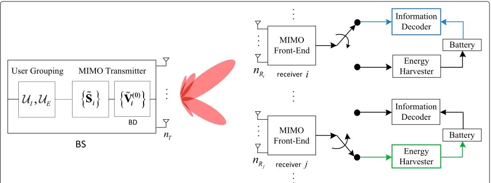
where thekth receiver is equipped withnRk antennas, as depicted in Fig.1.
We index frames byt ∈ T {1,. . .,T} with a dura-tion ofTfseconds each. We assume block fading channels,
that is, the channels remain constant within a frame but change from frame to frame. The equivalent baseband channel from the BS to the kth receiver is denoted by
Hk(t) ∈CnRk×nT. It is also assumed that the set of
matri-ces{Hk(t)}is known to the BS and to the corresponding
receivers. The case of imperfect CSI is beyond the scope of the paper.
The set of users is partitioned into two subsets, as men-tioned in the introduction. One of the sets contains the users that receive information, denoted asUI(t)⊆UTand
|UI(t)| =N, and the other set,UE(t)⊆ UT,|UE(t)| =M,
contains the users that harvest energy from the power radiated by the BS, which is used to transmit signals to the information receivers. Note that the previous sets depend ont, as the specific users in each of them may change from frame to frame. The numbers of users in each set,Nand M, may change from frame to frame as well, as will be explained later in the paper. We assume that a given user is not able to simultaneously decode information and har-vest energy. This forces a user to either receive informa-tion or harvest energy during the whole frame, i.e., during the scheduling period, which is a reasonable choice if the scheduling periods are short. That translates into disjoint
Table 1Notation used in the paper
A Set
A= {a1,a2,. . .} SetAcontaining the elements{a1,a2,. . .} |A| Number of elements in setA
a∈A abelongs to setA
A\a Set resulting from subtractingafrom setA
∅ Empty set
A⊆B SetAis included in or equal to setB
A∩B,A∪B Intersection of setsAandB, union of setsAandB
a,A Vectora, matrixA
aT,AT Transpose of vectora, matrixA
aH,AH Hermitian (transpose conjugated) of vectora, matrixA Tr(A), det(A) Trace of matrixA, determinant of matrixA
A0 MatrixAis positive semidefinite
||a|| Norm-2 of vectora
Cm×n Set of complex matrices of sizem×n In Identity matrix of sizen×n
E[·] Expectation
=,,= Equal, equal by definition, different
>,≥,<,≤ Higher, higher or equal, lower, lower or equal log(·), exp(·)=e(·)Logarithm, exponential
n! Factorial ofn
Summation
min, max Minimum, maximum
(x)b
a (x)ba=min{max{a,x},b} ab atob
∀ For all
maximizex1,x2,... Maximization with respect to variablesx1,x2,. . .
minimizex1,x2,... Minimization with respect to variablesx1,x2,. . . x Optimum value ofx
f−1(·) Inverse function x←y xis updated withy
subsets, i.e.,UI(t) ∩UE(t)= ∅,|UI(t)| + |UE(t)| ≤K.1To
simplify the notation when needed, we will assume that the indexing of users is such thatUI(t)= {1, 2,. . .,N}and
UE(t)= {N+1,N+2,. . .,N+M}.2We will assume that
nT >nR−mink{nRk}is fulfilled, beingnR=
k∈UInRk. 3
As far as the signal model is concerned, the received sig-nal for theith information receiver at thenth time instant within thetth frame can be modeled as:
yi(n,t)=Hi(t)Bi(t)xi(n,t)+Hi(t)
k∈UI(t)
k=i
Bk(t)xk(n,t)
Fig. 1Broadcast multiuser system. Schematic representation of the downlink broadcast multiuser communication system. Note that each user can switch from an information decoder receiver to an energy harvester receiver. This switching can be implemented technologically, as mentioned in papers such as [51]
In the previous notation, Bi(t)xi(n,t) represents the
transmitted signal for user i ∈ UI(t), where Bi(t) ∈ CnT×nSi is the precoder matrix, andx
i(t) ∈ CnSi×1
rep-resents the information symbol vector. nSi denotes the number of streams assigned to user i ∈ UI(t), and we
assume that nSi = min{nRi,nT − −(nR − −nRi)} ∀i ∈ UI(t) is fulfilled4. The transmit covariance matrix is Si(t) = Bi(t)BHi (t) if we assume, without loss of
gener-ality (w.l.o.g.), thatExi(n,t)xHi (n,t)
= InSi.wi(n,t) ∈ CnRi×1denotes the receiver noise vector, which is
consid-ered white and Gaussian withEwi(n,t)wHi (n,t)
=InRi5.
Note that the middle term of (1) is an interference term usually known as multiuser interference (MUI).
Letx˜(n,t) =B(t)x(n,t)denote the signal vector trans-mitted by the BS, where the joint precoding matrix is defined as B(t) =[B1(t),. . .,BN(t)]∈ CnT×nS, where
nS = Ni=1nSi is the total number of streams of all information users, and the data vector is x(n,t) =
xT1(n,t),. . .,xTN(n,t)T ∈ CnS×1. x˜(n,t) must satisfy the power constraint formulated as E˜x(n,t)2 =
N
i=1Tr(Si(t))≤PT, wherePT represents the total
radi-ated power at the BS, assuming that the information sym-bols of different users are independent and zero-mean.
Let us model the total power harvested by thejth user during thetth frame, denoted byQ¯j(t), from all
receiv-ing antennas to be proportional to that of the equivalent baseband signal, i.e.,
¯
Qj(t)=ζj
i∈UI(t)
EHj(t)Bi(t)xi(n,t)2
, ∀j∈UE(t),
(2)
where ζj is a constant that accounts for the loss in the
energy transducer when converting the harvested power
to electrical power to charge the battery. Note that, for simplicity, in (2), we have omitted the harvested power due to the noise term or other external RF sources since they can be assumed negligible. Based on this, (2) can be written as:
¯
Qj(t)=ζj
i∈UI(t)
TrHj(t)Si(t)HHj (t)
, ∀j∈UE(t).
(3)
For the sake of clarity, we will drop the time and frame dependence whenever possible.
2.2 Power consumption models
The energy consumed by the transceiver can be mod-eled as the energy consumed by the front-end plus the energy consumed by the coding/decoding stages (omitting for the moment the power radiated by the transmitter).6
Although other works consider battery imperfections in their models [28], we do not consider them in our work for the sake of simplicity. Note, however, that the strategy and formulation presented in this paper could be extended easily to incorporate those imperfections. In the following, we will comment briefly on the generic abstract approach followed in this paper to make the proposed strategies independent of the concrete model.
1. Front-end consumption: as far as the transmitter is concerned, the components that consume energy are the high-power amplifier (HPA), the mixers, the filters, and other elements of the RF chain.
received power [29], an operation that requires some additional power). In the following, however, we assume that the component of the receiver front-end consumption that depends on the SNR is negligible, as it can be concluded from the experimental measurements and is adopted in most works [29]. We denote the energy consumed by the front-end at the transmitter and the receiver byPtx
c andPcrx,
respectively.
2. Coding/decoding consumption: it is reasonable to consider the energy consumed by the coding stage at the transmitter negligible compared to the energy consumed by the front-end. This is illustrated and commented on in papers such as [30]. For this reason, we will not include coding consumption in our models. On the other hand, the decoding consumption must be included in the models since, as shown in [31] and [32], such energy consumption is not negligible and can affect importantly the lifetime of the mobile terminal. There is a consensus about the fact that the decoding consumption increases with the data rateRi(t),Pdec,i(Ri(t)). In
[33], the authors presented different models for Pdec,i(Ri(t)), but for the sake of generality, we will
consider it a general function.
Given the previous models, the total consumption at the transmitter (omitting for the moment the radiated power) only includes the front-end consumption as mentioned previously, and it therefore is denoted as:
Ptx
tot=Ptcx. (4)
On the other hand, the total power consumption at the ith receiver is expressed as:
Prx
tot,i(Ri(t))=Pdec,i(Ri(t))+Pcrx. (5)
Note that the power consumption at the receiver is limited by the current battery level, which in the following will be denoted byCi(t)for useri. According to this, the data rate
of a given information user (useri) during one frame must be constrained in order not to consume more energy when decoding than the current energy available at the battery Ci(t). Hence,
Tf(Pdec,i(Ri(t))+Pcrx)≤Ci(t), (6)
which can be written in terms of a maximum rate con-straint as:
We consider that each user terminal is provided with a finite battery capacity, the level of which decreases accord-ingly when the user receives and decodes data. The termi-nals are also able to recharge their batteries by means of collecting the power dynamically coming from the BS.
The battery at the beginning of thetth frame of theith information user served with a data rateRi(t−1)during
the previous frame is denoted as:
Ci(t)= tery level, and the functionPrx
tot,i(Ri(t−1))was defined in
(5). Note thatCi(t)has units of Joules.
On the other hand, the battery at the beginning of the tth frame of thejth harvesting user is denoted as:
Cj(t)=
The receivers must inform the BS about their battery level status to make decisions on whether to serve that user with information or with power. In this paper, we assume that the feedback channel is ideal and not rate-limited.
The power consumption and battery dynamics models, which are based on the state of the art and existing litera-ture, were also used in a similar way by the same authors of this paper in their previous work [33].
3 Joint resource allocation and user grouping formulation
In this section, we formulate the joint design of the covari-ance matrices Si(t), the data rates Ri(t), and the user
groupingUI(t),UE(t), based on the maximization of the
weighted sum rate with individual power harvesting con-straints for all time instantst∈T. Given this, the problem is formulated through the following optimization problem (this formulation generalizes the problem defined in our previous conference paper [1]):
C1 :
rate of theith user when considering linear precoding fol-lowing a BD strategy [25],Qj= set of minimum power harvesting constraints, andPmax
is the available power at the BS. In fact, BD is applied through constraint C5, which forces the complete can-cellation of the MUI, making the whole problem more tractable (as will be shown later in the paper). Notice that constraintC1 is associated with the minimum power to be harvested for a given user. In the case that another exter-nal energy harvesting source was available and the amount to be harvested could be estimated (or was fully known in advance), we could subtract such value fromQj
accord-ingly. Constraint C4 assures that the information users do not spent more energy decoding the message than the current energy available at the battery.
As we have already noted, we have assumed a linear precoding approach in the system formulation. Note that the optimum transmission policy in an MIMO broadcast channel is the well-known nonlinear dirty paper coding strategy [24]. Nevertheless, that strategy has high compu-tational demands and cannot be implemented in real time. Instead, much simpler linear transceiver designs have also been shown to achieve high capacities using much lower computational resources (see [34] for more details). Thus, for simplicity in the transmitter design, in this work, we force the precoder to be linear.
Two main difficulties arise when attempting to solve (10). First, note that the solution for all time instants has to be found jointly. The reason is that resource alloca-tion decisions at framethave an impact not only on that frame but also on future frames. Some researchers have attempted to solve harvesting (time-coupled) problems by assuming that the whole channel and harvesting realiza-tions are known a priori, giving rise to offline approaches that are not implementable in real scenarios [35,36]. As we assume that only causal knowledge of the channel and the harvesting is available, we would have to resort to dynamic programming (DP) techniques [37] to find the
optimal solution of the problem (10). However, these tech-niques usually require the implementation of extremely high-complexity algorithms that are impractical in scenar-ios, where the set of variables to be optimized is large, and DP techniques therefore have been applied only in cases where the optimization variables are scalars [38,39]. The second difficulty that we find is that the user grouping must also be optimized jointly with the covariance matri-ces and the data rates. The user grouping variables are discrete, and the problem therefore becomes combinato-rial. The optimum solution has to be found by applying some sort of combinatorial search among all possible user groups, increasing the overall complexity exponentially.
Because we are interested in low-complexity solutions, we have to make some simplifications to problem (10) to make it more tractable, with the hope of finding a good suboptimum solution that is close to the global optimum solution of problem (10).
The first assumption that we consider is to decouple the problem in time and propose a separate per-frame optimization approach. With this approach, we solve the optimization problem at the beginning of each frame t, making decisions based on the current and past informa-tion on the battery levels. The optimizainforma-tion to solve is (we omit the time dependence for the sake of simplicity in the notation even though all these variables, including the information and harvesting users setsUI andUE, change
at each frame) as follows:
maximize
Problem (11), which generalizes the one addressed in our previous paper [1], as weights are included to take into account the time evolution of the achieved rates, is still very difficult to solve, as it involves continuous and integer variables. Note that for a fixed set of groups,UI andUE,
problem (11) is convex with respect to{Ri,Si}and can be
solved using standard optimization techniques. The opti-mum solution can be found by solving problem (11) for all possible combinations of user groups, that is, an exhaus-tive search should be implemented. Consider for example that |UI| = 4 and |UE| = 4 and that K = 10. Then,
K!
|UI|!|UE|!(K−|UI|−|UE|)! =3.150 times. Clearly, the optimum solution is impractical, even for a system with a small number of users. In that sense, any technique aside from the exhaustive search may be suboptimal.
This fact motivates our second simplification: we decou-ple the decision of resource allocation and user grouping and propose a two-stage design strategy in which the user grouping is found based on suboptimal but less com-plex techniques. In other works, at the beginning of each frame, we first find the user groupsUI andUE, and then,
for those fixed user groups, we solve the following convex optimization problem:
Note that due to C5, problem (12) is convex; otherwise, the objective function, i.e., the weighted sum rate, would not be convex due to the MUI.
In the next section, we are going to present a method to solve problem (12) for different settings. Later, in Section5, we will present the user grouping techniques.
4 Weighted sum rate maximization with harvesting constraints
The problem presented in (12) is convex and can be solved using numerical interior point methods [40]. However, those methods usually have high computational complex-ity, and since we aim at finding a low-complexity solution, a customized algorithm should be developed. In some cases, it is possible to obtain the structure of the transmit covariance matrices in closed form and then develop an efficient algorithm based on that structure. Unfortunately, it is not possible to find the closed-form expression of the optimal transmit covariances for the previous problem due to the constraintC4. However, as we will show later, it is possible to find the transmit covariance structure of problem (12) ifC4 is not active.
To guarantee that constraint C4 is not active, we will assume that the set of information users is selected by the scheduler in the first stage in a way that they have enough battery such thatRi(t) < Rmax,i(Ci(t)),∀i ∈ UI
can be guaranteed in that particular scheduling period (later, we will comment on what to do in the unlikely event of violating the previous requirement). This is a reason-able assumption since users who have very low batteries should not be selected to receive information but to har-vest energy. Due to the previous simplifying assumption, constraintC4 will not be active, and we therefore do not consider it in the optimization problem. This assumption considerably simplifies the resolution of the problem.
Note that constraintC5 from the original problem (12) forces the precoder matrix Bi to lie in the right null
space of H˜i = contains the right-singular vectors in the null space of
˜
Hi. Thus, Bi can be written as Bi = ˜V(i0)B˜i (with
˜
Bi ∈ C(nT−nR+nRi)×nSi), and then, Si = ˜V(i0)S˜iV˜(i0)H,
where S˜i = ˜BiB˜Hi . Now, the optimization problem can
be rewritten in terms of the new optimization variables {˜Si}. Let Hˆi = HiV˜i(0) and Hˆji = HjV˜(i0). Note that
if constraint C4 is not present in (12), constraint C3 is tight at the optimum, i.e., Ri = log det
I+ ˆHiS˜iHˆHi
, and thus, the objective function is directly expressed as i∈UIωilog det
I+ ˆHiS˜iHˆHi
. Then, problem (12) (without consideringC4) is reformulated as
maximize
The problem above can be checked to be convex since the objective function is concave and the constraints define a convex set. As a consequence, there exists a global optimal solution that can be obtained numerically by means of, for example, interior point methods [40]. However, due to the fact that (13) is convex and satisfies Slater’s conditions [40], the duality gap is zero, and the problem, therefore, can be solved using tools derived from the Lagrange duality theory, and the optimal structure of the transmit covariance matrices{˜Si}can be revealed. Let
λ = {λj}j∈UE be the vector of dual variables associated with constraintC1 andμbe the dual variable associated with constraintC2. The optimal solution of problem (13) is given by the following theorem in terms ofλandμ.
Theorem 1The optimal solution of problem (13) has
andDˆi = diag
ProofSee Appendix1.
Note the similarities in the precoder structure between the result presented in (14) for the multiuser case and the result found in [9] for the single-user case. In the mul-tiuser case, we have to find a set of multipliers associated with the per-user harvesting constraints, which makes the problem more complex to solve. Finally, the optimum data rate achieved by useriis thus:
Ri=log det
However, the above process is still pending the com-putation of the optimal dual variables since we assumed in the previous development that the dual variables were given (in Theorem1, matrixAi depends on the optimal
values of the Lagrange multipliers). As long as we have a closed-formed expression of the covariance matrices ˜
Si(λ,μ)as a function of the dual variables, we can solve
the dual problem of (13) by maximizing the dual func-tiong(λ,μ)subject toλ 0,μ ≥ 0, and Ai 0∀i.
This can be addressed by applying any subgradient-type method, such as, for example, the ellipsoid method [41]. It can be shown that the subgradient ofg(λ,μ), denoted ast,
which represents the subgradient ofg(λ,μ)with respect to λm andμ, respectively ([t]k denotes the kth entry of
vectort), andS˜i is computed as in (14) for a givenλand μ(for each step of the algorithm, we computeS˜ijust by
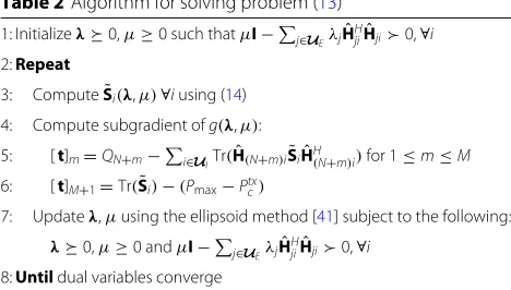
replacing, in expression (14), the optimal values of the Lagrange multipliers by their current values). Since the duality gap is zero, when we obtain the optimal dual vari-ables (λ andμ) with the ellipsoid method, the optimal solutionS˜i(λ,μ)converges to the primal optimal solu-tion of problem (13). As a summary, the algorithm that solves problem (13) is described in Table2(this table was already presented in [1] but is included here for the sake of completeness).
4.1 Particular cases: scenario with only one type of user There exists a couple of particular cases of the problem presented before in which only one type of user is present in the system. Such simplified scenarios are found in real systems and will yield simpler optimization problems with lower computational complexity in the resolution of the
Table 2Algorithm for solving problem (13)
1: Initializeλ0,μ≥0 such thatμI−j∈U
7: Updateλ,μusing the ellipsoid method [41] subject to the following: λ0,μ≥0 andμI−j∈UEλjHˆHjiHˆji0,∀i
8:Untildual variables converge
resource allocation algorithm. For the sake of ease of read-ability of the paper, the mathematical developments of both particular cases have been moved to AppendixC.
4.2 Trade-off analysis between weighted sum rate and power constraints
In this section, we analyze the multidimensional trade-off between the objective function, that is, the weighted sum rate, and the set of power harvesting constraints. For simplicity, let us consider thatCi(t)∀i ∈ UI is high
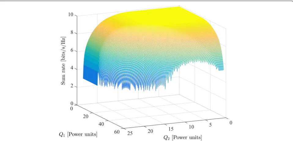
. We would like to emphasize that, as the noise and channels are normalized, we will refer to the powers harvested by the receivers in terms of power units instead of Watts. Given this approach, we propose to use therate-power(R-P) region to characterize all the achievable sum rates (in bit/s/Hz) and power har-vesting (in power units)M+1-tuples under a given power constraint as in [9]. The R-P region of problem (13) is
To be able to graphically show an example of the trade-off, we restrict the cardinality of the set of harvesting users and information users to be two, i.e.,|UE| =2 and
|UI| =2, and for simplicity, we consider thatωi=1, ∀i∈
UI. In such a case, the trade-off region between the sum
rate and the two power constraints is a three-dimensional surface. The setup taken as an example for this section is a BS with four transmit antennas and where all users have two antennas. The maximum transmission power at the BS isPmax−Pctx = 10 W. The entries of the matrix
Fig. 2Three-dimensional R-P region. Representation of the three-dimensional R-P region of problem (13). The figure represents the existing trade-off between the optimal solution of the problem, i.e., the weighted sum rate, and the two power harvesting constraints
Figure2 depicts the three-dimensional R-P region for the previous setup. As can be appreciated, the opti-mal sum rate solution is jointly concave on Q1 and
Q2, as expected [40]. The values of Q1 and Q2 for
which the region is not defined correspond to situations where problem (13) is infeasible. To characterize the
surface accurately, let us introduce the contour lines of the R-P region in Fig. 3. In the plot, when the lines are close together, the magnitude of the gradi-ent is large. There are also some important boundary points marked in the 3D plot of the surface. Those points can be computed in a simple way and provide
us with useful cases that will be commented on in what follows.
Let us first start with the boundary point defined by
(SRmax, 0, 0). The power harvesting constraints for users
1 and 2 at this point are set to zero, and the solution of the problem therefore can be obtained from problem (22) (or from problem (13) withQ1 = Q2 = 0). SRmax
repre-sents the maximum sum rate that can be achieved in this situation when no energy harvesting is imposed. The opti-mum covariance matrices were obtained in Section 4.1 and are denoted here as S˜SR
i for the ith user. Fol-lowing that notation, the maximum sum rate can also be expressed as SRmax = log det
Note that although when computing SRmaxwe do not
apply power harvesting constraints, this does not neces-sarily mean that the actual harvested powers are zero. In this context, we have the boundary point(SRmax,QI1, 0),
where QI1 represents the power harvested by user 1 when the precoder matrices are the ones that maximize the weighted sum rate, i.e., QI1 = Tr
. The same can be said for the
bound-ary pointSRmax, 0,QI2 , whereQI2=Tr
. Then, there is a fourth point that defines a flat surface (or tableland) of constant sum rate SRmax, which is the combination of the two previous
points,SRmax,QI1,QI2 . In other words, the tableland of
constant maximum weighted sum rate SRmax defines all
possible values of harvested power constraints for which constraintsC1 are not active and thus do not affect the optimum value of the weighted sum rate.
Now, let us consider the boundary points in terms of maximum harvested power. On top of the figure, there is the point(SRE1,Q1,max,Q12). This point corresponds to the
situation in which the power harvested by user 1 is a max-imum or, in other words, the maxmax-imum value ofQ1for
which problem (13) is feasible, assuming no constraint on the power to be harvested by user 2. To calculateQ1,max,
we solve the following optimization problem:
maximize
whereS˜E1represents the sum of the two covariance
matri-ces for the information users (note that in this problem, the objective function and the constraint depend on such matrices through their sum), and the objective function is the power harvested by user 1. Now, by applying the result from Proposition 2, we obtain the solution of problem
(17) as follows. Let the reduced eigen-decomposition of ˆ
HH11Hˆ11beUˆ11ˆ11UˆH11such thatuˆ11,maxis the eigenvector
associated with the maximum eigenvalue λˆ11,max. Then,
the solution to the previous problem is based on the fol-lowing inequality: Tr Pmax − Ptxc), where such inequality becomes equality if
˜
SE1 = Pmax−Ptxc × ˆu11,maxuˆH11,max. In this case, the
maximum harvested energy is accomplished by energy beamforming9(i.e., rank 1) to the best eigenmode of the
equivalent channel HˆH11Hˆ11. Then, we obtain Q1,max =
TrHˆ11S˜E1HˆH11
= (Pmax − Ptxc) × ˆλ11,max. According
to this, the weighted sum rate obtained by solving prob-lem (13) andQ1 = Q1,max,Q2 = 0 (denoted as SRE1) is Note that, even though we do not apply the power har-vesting constraint of user 2 when computingS˜E1, it does
not mean that the actual power harvested by user 2 is zero. In this context, we define the last coordinate of the point, denoted asQ12, which represents the power harvested by user 2 when the covariance matrix is S˜E2, i.e., Q12 = TrHˆ21S˜E2HˆH21
. The same reasoning can be applied to obtain the last boundary point(SRE2,Q21,Q2,max)by
inter-changing the roles of users 1 and 2.
The remaining boundary points in the curve can be obtained by properly varying the values of Q1 and Q2
(0≤Q1≤Q1,max, 0≤Q2≤Q2,max) in problem (13).
5 User selection policies
Thus far, we have assumed that the two groups of users, i.e.,UIandUE, were known. The goal of this section is to
propose a grouping strategy to select which users should go into each set in a way that the aggregated through-put over time is maximized. As the channels and batteries fluctuate throughout time, the users in each group may also change from frame to frame. In this section, we will assume that the values of{Qj}are known and fixed. The
management of these values is beyond the scope of the paper (see the work in [43], where the authors propose some procedures to adjust the values of{Qj}, considering
the impact on the system performance).
techniques for the user grouping for both kinds of users, i.e., information and harvesting users. This is one of the major contributions of our paper, that is, work with users that have different objectives. Additionally, as we will show, the proposed greedy algorithms take into account that the selection of the harvesting users impacts directly the performance of the information users, that is, there is a coupling behavior between both aspects.
The overall user grouping strategy will be divided into two stages. In the first stage (that will be known as super-grouping), we will provide a preselection of user candi-dates to be in each set. This will depend primarily on the current energies available at the batteries, and it will be run at a longer time scale, every few scheduling periods or frames. For the second stage, known asgrouping, we are going to present two different user grouping strate-gies that will be run at every frame. The strategy with the highest complexity provides a better performance than the simpler strategy.
In the first (simpler) approach, we will split the user grouping further into two stages. The first stage selects the information users,UI, from the supergrouping setUIS
based on a greedy approach, whereas the second stage selects the harvesting users, UE, based on the already
selected information users. In the second approach, we will develop a joint information-harvesting group-ing strategy, which constitutes an intermediate approach between the first simple approach and the optimum approach based on exhaustive search.
5.1 User supergrouping strategy
Recall that when we derived the optimal precoder matrix in Section4, we assumed that the optimal rates would ful-fill Ri(t) < Rmax,i(t), ∀i ∈ UI for any particular frame,
and therefore, constraints C4 in problem (12) were not active. This is achieved by preselecting the users that are to be scheduled for data transmission or battery charging. In our proposed approach, we first implement a selection of candidates to be inUI andUE, known asUISandUES,
such thatUI ⊆ UIS,UE ⊆ UES, andUIS+UES = K, and
we then select the users that finally go into the setsUIand
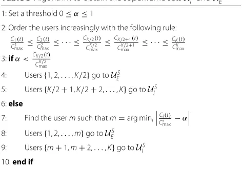
UE. The proposed supergrouping algorithm is presented
in Table3and works as follows: we set a thresholdαsuch that 0≤α≤1. Then, we compute the ratio of the current battery level and the battery capacity for all users, and we then order these ratios increasingly. If the middle ratio of the previous list is greater than the value of the threshold
α, we then split the overall group by half and put half of the users inUISand the other half inUES. On the other hand, if the middle ratio of the previous list is lower than the value ofα, we find the user with battery ratio closest to the value ofαand put all users with lower ratios than the one clos-est toα in the harvesting set and the remaining users in the information set. The larger the value ofα, the greater
Table 3Algorithm to obtain the superframe setsUS I andUES 1: Set a threshold 0≤α≤1
2: Order the users increasingly with the following rule: C1(t)
the number of users that will be included in the harvest-ing setUES. Note that the BS has to know the battery levels of all users, which implies that receivers must send the battery levels through a feedback channel and, hence, the battery levels must be quantized (in [33], we addressed the problem of quantizing the battery levels and evaluated the effect on the overall system performance, and we conclude that a few bits for quantization is enough to obtain good performance).
5.2 Disjoint information and harvesting user grouping This first approach is based on two stages. In the first stage, the selection of the information users follows a greedy approach, in which each user is added at a time and the maximization of the weighted sum rate without harvesting constraints is evaluated for all possible candi-date information users with the already selected users. No harvesting users are considered at this stage.
Let us assume, for simplicity, that every information user has the same number of antennas, i.e.,nRi =NR,∀i∈ UT. The maximum number of simultaneous users to be
served following the BD strategy is then U = nT
NR
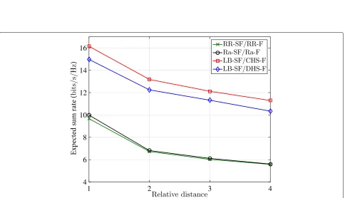
[25]. The algorithm for selecting the information users is shown in Table4; first, we select the user that can achieve the greatest weighted rate10. Then, we incorporate one
user at a time into the set only if the accumulated weighted sum rate increases due to incorporating such a user (weighted sum rate evaluated with the already selected users). The algorithm ends when there is no improvement in the weighted sum rate or when the maximum number of users to be scheduled (U) is reached.
Note that the distances from the BS to the users are taken into account implicitly in the algorithm since in step 2 and step 8 of Table4, we select users according to the rates. These rates depend on the channel matrices{Hi},
Table 4Algorithm to obtain the set of information usersUI
Once we have selected the information users, we con-tinue with the selection of the harvesting users in the second stage of this grouping strategy. The idea is to select the harvesting users so that when the resource alloca-tion strategy is executed, they affect (reduce) the system performance as little as possible (see Section 4.2). Let
S = i∈UISi, where UI and {Si}i∈UI are the infor-mation user set and the optimum covariance matrices obtained from the algorithm detailed in Table4, respec-tively. The algorithm works as follows. For each harvesting userj, we evaluate and decreasingly order Tr(HjSHj)−
Qj and select the first M harvesting users according to
this order. Note that in the previous expression, we are evaluating how the optimum covariance matrices of the selected information users transmit power in the geomet-rical direction of the channels of the harvesting users. We also take into account the minimum required power to be harvestedQjto ensure feasibility of the solution of the
resource allocation problem. The algorithm is presented in Table5.
5.3 Joint information and harvesting user grouping In this second approach, the selection of the informa-tion and harvesting users is coupled. Due to this joint
Table 5Algorithm to obtain the set of harvesting usersUE
1:Input:UItaken from algorithm in Table4,S=i∈UISi, 2:Evaluatemj=Tr(HjSHj)−Qj, ∀j∈UES
3:Decreasingly ordermj
4:ConstructUEwith the users corresponding to the firstMordered terms ofmj
approach, the system performance will be degraded less by the effect of having harvesting users in the system com-pared with the previous decoupled approach. However, the computational complexity increases as more combi-nations need to be evaluated.
The algorithm for selecting the information users is based on the same greedy approach that we presented before. The difference is that, now, instead of selecting the information users and then the harvesting users, we select both types of users simultaneously. For simplicity in the formulation, let us consider thatMis an integer multiple ofU and definek = MU (we will comment later on how we could apply the algorithm if that was not the case). The idea behind the algorithm is as follows. We select one information user q and obtain its optimum covari-ance matrixSq. Then, we find the bestkharvesting users based on the principle developed in Table 5. After that, we select another information user and repeat the same process until there is no improvement in the objective function. Due to the fact that the grouping is coupled, we consider the impact of having selected harvesting users on the future selection of information users. The specific details of the joint algorithm are presented in Table6.
Table 6Algorithm to jointly obtain the set of information and
harvesting usersUI,UE
The main difference with the algorithm in Table 5 is that, now, we solve problem (13) with constraintsC1, that is, with harvesting users, which increases the complexity of the overall grouping procedure. As addressed before, if Mis not an integer multiple ofU, we can introduce more harvesting users in step 21 in Table6in some iterations, e.g., ifM = 7 andU = 3, we first select three harvest-ing users and then two harvestharvest-ing users in the other two iterations.
6 Overall user grouping and resource allocation algorithm
In the following, we present a summary of the overall algo-rithm that consists of the user supergrouping, the user grouping, and the resource allocation stages presented in the previous two sections. Note that the user super-grouping is carried out every few frames, whereas the user grouping is executed at each frame. If, for some rea-son, the supergrouping algorithm fails in fulfillingRi(t) < Rmax,i(t),∀i∈UI(an event that would be unlikely to
hap-pen), then for those users for whichRi(t)≥Rmax,i(t), we
just transmit information in some channel accesses of the frame until their battery is over. The overall algorithm is detailed in Table7.
7 Results and discussion
In this section, we perform some numerical analysis of the proposed grouping and resource allocation strategies. The system comprises one transmitter with 8 antennas and 30 users(|UT| =30)with 2 antennas each. The
maxi-mum radiated power isPmax=11 W, and the transmitter
front-end consumption is Ptx
c = 1 W. Front-end power Table 7Overall user grouping and resource allocation algorithm
Beginning of a superframe:
1: Runuser supergroupingalgorithm in Table3: obtain setsUS I andUES Beginning of each frame (two options):
Option 1:
2a: Runinformation user groupingalgorithm in Table4: obtain setUI 2b: Runharvesting user groupingalgorithms in Table5: obtain setUE 2c: Runresource allocationalgorithm in Table2
Option 2:
3a: Runjoint information and harvesting groupingalgorithm in Table6: Obtain setsUIandUE
3b: Runresource allocationalgorithm in Table2
End of each frame:
5: Update weights (e.g., using a PF approach): wi(t)=Ti(1t), Ti(t)=
consumption at the receiver is Prx
c = 100 mW, and the
model used for decoding is exponential, i.e., Pdec(R) =
c1ec2R, wherec1=30, andc2=0.75 [33]. The frame
dura-tion is equal toTf =100 ms, and the superframe duration
is equal to 3 s. The channel matrices are generated ran-domly with i.i.d. entries distributed according toCN(0, 1). The noise power is normalized to 1. The effective window length for the PF scheme isTc = 5. The percentage used
for supergrouping isα = 0.1. The battery capacities are generated randomly from 3000 to 10,000 energy units. As we mentioned previously, we assume that all the harvest-ing constraints are the same for all users and fixed for all periods toQj = 50 power units, unless stated otherwise.
A strategy on how to manage and dynamically adjust the values of the{Qj}was proposed in [43] and is beyond the
scope of this paper.
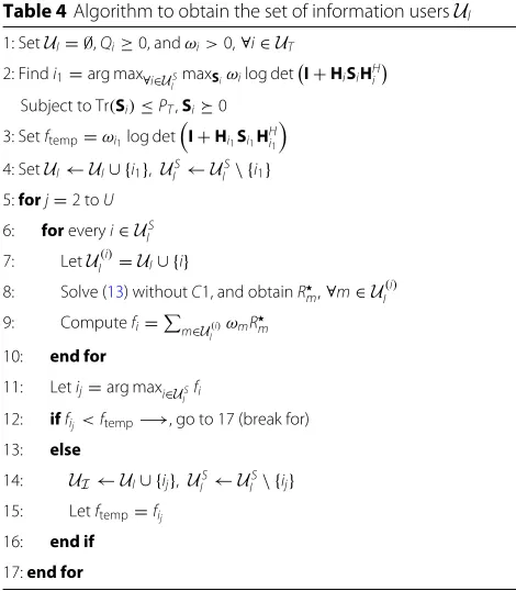
In the simulations, we compare our proposed two meth-ods with two other schemes. As there are no propos-als in the literature for user scheduling in the SWIPT framework, we compare our approaches with traditional schemes. In one of the schemes, we assume that the super-grouping and super-grouping are implemented with a round robin strategy. We will denote this strategy RR-SF/RR-F. In the other scheme, we consider that random selection of users is implemented at both levels as well. This strat-egy will be denoted by Ra-SF/Ra-F. On the other hand, the proposed supergrouping strategy (Table3) will be denoted by LB, and the grouping will be denoted according to the algorithm: DHS for the decoupled approach presented in Section 5.2(Tables 4and 5) and CHS for the approach presented in Section5.3(Table6).
7.1 Time evolution simulations
Fig. 4Time evolution of the battery levels. Time evolution of the battery levels of all users in the system for the different approaches
Figure5 presents the average sum rate of the system (computed as SR(τ) = 1ττt=1i∈UIRi(t)). This
met-ric is an estimation of the expected throughput of the system. From the figure, we see that the sum rate of the round robin and random schemes provides a stable average throughput over time but the magnitude of the
throughput is not so high. Then, we see how the proposed schemes notably outperform the previous benchmarking strategies. The simpler approach, DHS, performs similar to the more complex strategy, CHS. We also plot, as benchmarks, two cases. The first one, called “no har-vesting management,” refers to the case in which the
harvesting users are selected jointly with data users fol-lowing the CHS approach, but their harvesting constraints are set to zero,Qj = 0,∀j, that is, harvesting users
col-lect energy without imposing a constraint. In this case, the rate achieved is higher at the beginning, but the energy collected by the users is lower, having an impact on the performance as time goes on. The second case consid-ers that no power transfer (no SWIPT) is available, and users therefore cannot recharge their batteries. In this case, the users run out of battery, and the expected sum rate therefore tends to zero.
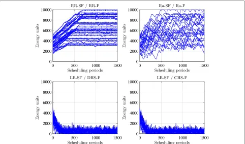
Figure 6 shows the cumulative distribution function (CDF) of the individual data rates of the users in the sys-tem. The CDF of the no SWIPT case has a particular shape due to the fact that many users obtain zero data rate as they run out of battery. In this figure, we clearly see the benefits of the proposed user selection schemes compared to the other approaches, such as low data rate percentiles and high data rate percentiles being much better for the proposed strategies.
Finally, in Fig.7, we depict the average evolution of the harvested power. It is interesting to note how all users tend to converge to a certain point (or the vicinity of a point). This is due to the fact that if a user is receiving much power, then its battery will increase, which will make the user more eligible to receive data, making the harvesting decrease, whereas if a user has low energy in its battery, then it is directly selected to be included in setUS
E. We
observe that the more complex approach, CHS, is able to provide the users with larger harvested power compared to the less complex approach, DHS.
7.2 System performance simulations
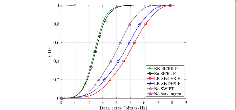
In the next figures, we will show the performance of the system obtained once the algorithms have converged (i.e., after 1500 frames). The first two figures, Figs. 8 and9, show the system performance, considering that half of the users are at a relative distance to the BS greater than for the other half of the users. In particular, Fig.8 presents the sum of the expected sum rate for the four schemes for four different relative distances. As expected, the sum rate decreases as the distance to the BS increases. On the other hand, Fig. 9 shows the sum of the expected harvested power as a function of the relative distance. We see that if half of the users are four times farther away from the BS, the loss in harvested power is from 25 to 50%, and the relative loss is lower for the proposed schemes.
The last two figures, Figs.10and11, show the perfor-mance of the system when the size of the harvesting group increases in relative terms when compared to the size of the information group, i.e., when MU increases. This phe-nomenon is interesting to evaluate since the harvesting users appear in the constraints and they negatively affect the aggregated sum rate (see trade-off in Section 4.2). However, if many users are introduced in the harvest-ing set, then their batteries will recharge faster, and they will be able to receive higher data rates. This is the com-promise that is analyzed in the figures. First, in Fig. 10, we see the expected aggregated sum rate. As we see, for the two benchmarking approaches, Ra and RR, the sum rate decreases as MU increases. This is because the har-vesting users are selected without considering the impact
Fig. 7Time evolution of the average harvested power. Time evolution of the average harvested power of all the users in the system for the different approaches (in power units)
Fig. 9Sum of expected harvested powers by all users vs distance to the BS. Sum of the expected harvested powers by all users (in power units) as a function of the distance to the BS
that they have on the objective function, and therefore, if more harvesting users are considered in the optimiza-tion problem, a lower sum rate will be achieved. In those cases, the optimization problem turns out to be infeasible many times, and therefore, the energy collected by all
users also decreases, see Fig.11. On the other hand, the aggregated sum rate increases a bit for MU = 2 for the proposed strategies. This is due to the fact that harvesting users are selected very efficiently, and thus, the constraints associated to them are not active, i.e., they do not affect
Fig. 11Sum of expected harvested powers by all users vs relative size of the harvesting user group. Sum of the expected harvested powers by all users (in power units) as a function of the relative size of the harvesting user group
the optimum value of the objective function. Additionally, as more users are able to recharge their batteries (see Fig. 11), they can decode higher rates in future frames. Nonetheless, from a given size MU on, the system sum rate starts to decrease as the harvesting constraints become active, although the problem is always feasible, and users recharge their batteries, as is indirectly depicted in Fig.11.
7.3 Computational complexity
An analytic evaluation of the computational complexity of the proposed techniques for each scheduling period is extremely difficult since these algorithms are itera-tive, each iteration involves the numerical solution of an optimization problem, there are discrete variables related to the grouping of users, and the solution and conver-gence times depend on the concrete channels associated to the users in the scenario. Because of this, we have per-formed a numerical evaluation of the computational com-plexity of the different algorithms by performing many simulations over random channels and averaging the con-vergence times at each scheduling period obtained in the simulator. Figure 12 shows a set of bars comparing the complexities needed for convergence of the different algorithms that require grouping, that is, RR-SF/RR-F, Ra-SF/Ra-F, LB-SF/CHS-F, and LB-SF/DHS-F. The highest bar corresponds to the algorithm requiring the high-est computational complexity, which is LB-SF/CHS-F and has been labeled as the 100% reference. The other bars show the complexities associated to the other algo-rithms, taking as relative reference, the complexity of LB-SF/CHS-F.
8 Conclusions
Fig. 12Relative computational complexities. Average computational complexities of each algorithm needed for convergence at each scheduling period relative to algorithm LB-SF/CHS-F
Appendix 1
The Lagrangian of problem (13) is:
L({˜Si};λ,μ)= −
where we have omitted constraint C3. The previous Lagrangian can be manipulated and transformed into:
L({˜Si};λ,μ)= −
Proposition 1To have a bounded solution of the dual
function g(λ,μ), matrixAimust beAi 0∀i; otherwise,
g(λ,μ)is unbounded below, i.e., g(λ,μ)= −∞.
ProofSee Appendix2.
Due to the fact that matrices {Ai} are positive
def-inite, we can assure that they can be decomposed as
Ai = A1i/2A1i/2and that they always have inverses. Thus,
The dual function in (20) can be recognized to be equiv-alent to the dual function of the classical maximization of the sum rate with a power constraint, where the opti-mum covariance matrix Sˆi diagonalizes the equivalent
channelHˆiA−1i /2[26], i.e.,Sˆi = ˆViDˆiVˆHi , whereDˆiis the
power allocation matrix, and its components are com-puted following the water-filling policy [49]. Finally, it is straightforward to show that the precoderBimatrix with
dimensions nT × nSi corresponding to such covariance matrix is:
Bi= ˜V(i0)Ai−1/2VˆiDˆ1i/2. (21)
Appendix 2
Let the eigen-decomposition of Ai be U¯i¯iU¯Hi , where
¯
i contains the eigenvalues in decreasing order w.l.o.g.
Then, the second term of the Lagrangian in (19) is
for the covariance matrix S¯i as being diagonal, with all