Evaluation of range based indoor tracking algorithms by merging simulation and measurements

R E S E A R C H

Open Access

Evaluation of range-based indoor

tracking algorithms by merging simulation

and measurements

Klemen Bregar

, Roman Novak

and Mihael Mohorˇciˇc

Abstract

Precise location information will play an important role in 5G networks, their applications and services, especially in indoor environments. Ultra-wideband (UWB) technology offers exceptional temporal resolution enabling the

emergence of high accuracy ranging-based indoor localization systems. In order to reduce time to market, developers need a reliable, fast and efficient method to evaluate localization and tracking system designs in the selected

high-dimensional parameter space. Purely measurement-based performance evaluation of such systems is costly and cumbersome, so we propose the use of a radio frequency (RF) ray-tracing simulator augmented with a noise model based on measurements with localization equipment in real environment. We demonstrate the proposed approach by evaluating the UWB-based two-way-ranging (TWR) localization with the least squares (LS) and with the extended Kalman filter (EKF) tracking algorithms. We analyze the degradation of tracking performance due to time spreading of range measurements. Moreover, on a set of fixed locations we also show that the proposed approach is sufficiently representative for the pure measurement-based evaluation. The results obtained in a reference office environment show that EKF algorithm is twice as efficient and more resilient to the effects of time spreading of range

measurements as LS algorithm.

Keywords: Indoor position tracking, Ultra-wideband, RF ray-tracing, Tracking algorithm evaluation

1 Introduction

Precise tracking and localization are gaining the impor-tance in modern applications and services and are among the key enablers of the 5G networks. They are addressing the challenges of application domains as well as sup-porting the optimization of network performance and improved utilization of radio resources in increasingly densified environments [1]. In outdoor scenarios, global navigation satellite systems (GNSS) augmented by terres-trial cellular and wireless network localization techniques provide sufficient precision and accuracy for most of the applications in 5G networks, they are considered mature and well-tested technology, and are readily available in most of the mobile devices available in the market already today.

*Correspondence:[email protected]

1_{Department of Communication Systems, E6, IJS, Jamova cesta 39, 1000}

Ljubljana, Slovenia

2_{Jožef Stefan International Postgraduate School, Jamova cesta 39, 1000}

Ljubljana, Slovenia

Many 5G application domains, however, depend on pre-cise location information also in the indoor environment, such as tracking the inventory, goods and people, navigat-ing robots, and autonomous drivnavigat-ing vehicles inside manu-facturing facilities, optimizing wireless network resources according to users’ demand.

In indoor environments, satellite signals are gener-ally too weak or degraded to be of any use. Different approaches with special infrastructure are thus used to serve the needs of indoor localization systems, their choice largely depending on the required localization accuracy, equipment availability, and deployment com-plexity. This localization infrastructure can be a part of the existing communication infrastructure (e.g., WiFi access points) or needs to be installed and maintained separately (e.g., Bluetooth beacons, NFC tags).

One approach for indoor localization and tracking sys-tems is based on signal propagation models. For good performance, these systems mostly rely on extensive mea-surements and calibration procedures [2, 3]. Another

promising approach for a precise and accurate indoor localization is based on the use of ultra-wideband (UWB) pulse radios developed especially for ranging applica-tions with time-of-flight (ToF) measurement capability. These do not require any calibration for a very accu-rate localization in line-of-sight (LoS) signal propagation conditions [4].

Regardless of the approach, developing reliable and accurate localization and tracking algorithms and espe-cially their performance evaluation require extensive and costly deployment of localization equipment and time-consuming measurement procedures. Moreover, it is dif-ficult to precisely track the moving object and also track the communication between the nodes while studying the impacts of all parameters (e.g., ranging time step, ranging sequence, movement speed) on a final tracking and localization performance. To this end, developers of localization and tracking algorithms need a suitable sim-ulation approach that is considering most of the aspects from the real operating environment. It should enable fast performance evaluation and investigation of the sensitiv-ity of tracking algorithms to various parameters such as speed of movement, ranging update period, localization resolution, computation time.

Radio frequency (RF) ray tracing is a particularly valuable technique in the development of wireless tech-nologies in indoor environments. It is based on a phys-ical channel model that allows far superior prediction of electromagnetic propagation effects than any other stochastic modeling, thus being able to accurately simu-late real operating environment from the signal propaga-tion perspective. Accuracy wise, it can only be surpassed by approximations of spatial and temporal derivatives appearing in Maxwell’s equations, but those are compu-tationally infeasible if the wavelength is exceedingly small compared to the size of the modeled environment.

In this article, we propose a simulation approach for evaluation of range-based tracking algorithms. The approach exploits the benefits of a controlled environ-ment of an RF ray-tracing simulator augenviron-mented with real environment measurements. This makes the approach able to investigate the sensitivity on the movement, rang-ing protocol, and geometry specifics, thus ensurrang-ing sim-ulator representability. We demonstrate the proposed approach in a reference office environment, modeled and imported in a RF ray-tracing simulation software together with all materials but without furniture. The measurement step in the selected environment intro-duces the noise which we model by the measurements obtained from actual ranging equipment, complement-ing the noise-free simulation environment to resemble the real-tracking system behavior. With the proposed sim-ulation approach, we then evaluate the performance of the simple least squares (LS) and the extended Kalman

filter-based (EKF) tracking algorithms with the constant velocity walking model on simulated trace-based ranging data. Such simulation approach ensures repeatability of results, non-obtrusive testing and validation of the sys-tem for people working in the target environment, and fast execution of multiple iterations in searching through the high-dimensional parameter space for optimal parameters setting.

The main contributions of this paper are

• A complete simulation-based approach exploiting realistic measurement-based noise model and models of a reference operating environment, movement of traced terminal, and ranging protocol.

• Evaluation of two reference localization algorithms for different parameter settings focusing on the impact of ranging noise, ranging update period, and walking path resolution.

The rest of this paper is organized as follows. Related work is presented in Section 2. Section 3 describes the proposed simulation-based approach and models used for evaluation of localization and tracking algorithms. In Section4, the selected reference tracking algorithms are described. In Section5, the performance evaluation of the reference tracking algorithms is given according to differ-ent parameter settings. Finally, Section6gives conclusions and outlines the future work.

2 Related work

The main lines of previous research work related to this study are concerned with indoor localization and RF ray-tracing simulation algorithms. Both lines have been exten-sively investigated in the research community, so we only provide very coarse overview of the related literature with the aim to position the proposed simulation approach for evaluation of ranging-based tracking algorithms.

2.1 Indoor localization

Indoor localization approaches can be classified accord-ing to the information they are based on to received signal strength indicator (RSSI)-based methods, angle-of-arrival (AoA)-based methods, and time-based localization methods [3].

and consequently great localization accuracy are desired [7]. In such environments, time-based localization meth-ods measuring the signal propagation time between a transmitter and a receiver provide a reasonable trade-off between the accuracy and implementation complexity. The baseline time-based localization and tracking algo-rithms rely on a precise clock synchronization between a transmitter and a receiver and calculate the range from time-of-arrival (ToA) or time-difference-of-arrival (TDoA) [3], so we refer to them also as range-based methods. For more general systems, where no time syn-chronization between nodes is available or feasible such as assumed in this article, dual-time-of-flight (DToF) or two-way-ranging (TWR) algorithms can be used [8]. This approach requires two-way communication between a tag (i.e., node with the unknown location) and all anchors (i.e., nodes with known locations). A message is exchanged at least two times between a tag and each anchor. The current local time stamp is pinned to a message every time it is received or transmitted as can be seen in Fig.1. After a full TWR cycle between a tag-anchor pair is completed, four timestamps are accumulated (Tpoll_TX, Tpoll_RX, Tresp_TX, and Tresp_RX) and local clock

differ-ences can be eliminated according to (1).

ˆ

TTWR=

Tround−Treply

2 , where

Tround =Tresp_RX−Tpoll_TX Treply =Tresp_TX−Tpoll_RX

(1)

This approach removes the need for time synchroniza-tion among the nodes, but relies on a suitable ranging protocol for contention resolution in a system with many tracked nodes and anchors. In case of tracking a moving object, the time required for collecting multiple times-tamps in turn to each anchor node introduces errors to the final estimated location since each anchor samples the location at different point in time and space.

2.2 RF ray-tracing

RF ray-tracing technique, adopted from the com-puter graphics domain, is increasingly used for radio environment characterization particularly in indoor envi-ronments. Many RF ray-tracing algorithms have been proposed since first ideas by Ikegami et al. [10] in 1991.

Advanced RF ray-tracing algorithms take into account the majority of paths the real wave-front would tra-verse and model actual physical phenomena responsible for propagation of electromagnetic waves, in particular reflection and refraction. From the ray handling perspec-tive, most of them fall into three computationally distinct groups. The first, often seen as the brute force approach and used in our simulation tool, effectively traces a large number of rays from the transmitting source in all direc-tions into the scene. The concept of a reception sphere is needed to detect rays passing by the receivers [11]. The algorithms from this group refer to the principle as ray launching [12], pincushion method [13], or ray shooting and bouncing (SBR) [14], which is also a designation used in this article. The second approach aggregates traced rays as ray tubes [15] or beams [16] in order to reduce com-putational complexity. Finally, the third RF ray-tracing approach [17] goes the furthest by using entire scene surfaces as ray aggregation units.

3 Methods

In this section, we present the entire setup of the RF ray-tracing-based simulation approach for the evaluation of tracking algorithms including the models of the ref-erence environment and movement, and the calibration measurement setup.

3.1 Reference environment model

As a reference environment for simulation and measure-ments, we selected an office environment which occupies the entire top floor in an office building of dimensions 15.38 m×11.5 m. It consists of eight offices, two toilets, a

hallway, and a staircase. The inner walls are made mostly of drywall material with a few reinforced concrete pillars supporting the roof.

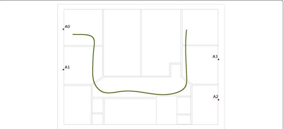
The complete environment including the wall and ceil-ing materials was modeled in a 3D modelceil-ing software and imported into a custom RF ray-tracing simulation soft-ware described in Section 3.2. The office environment floor plan is depicted in Fig.2.

Four anchor nodes with known locations are placed in the environment and a walking path for position tracking simulation is generated as described in Section3.3. Each point on a walking path has a unique set of ranging errors for range measurements to anchor nodes because each position in an environment has different signal propaga-tion condipropaga-tions. Ranging errors are mostly proporpropaga-tional to the number of walls and their thicknesses the ray propagates through along the signal path.

3.2 RF ray-tracing simulator

The proposed simulation approach can use any RF ray-tracing tool, but to avoid the potential influence or bias to results of any hidden details of the implementation and to have full control over all simulation parameters at the source code level we decided to use our own radio frequency ray-tracing simulator1. It was developed and validated in the course of several applied and indus-trial projects and is based on the brute force shooting and bouncing rays (SBR) for simulation of ToF measure-ments. The simulator has already been proven in sev-eral projects with the telecommunication industry. It is a highly optimized GPU-based ray tracer using the NVIDIA OptiX ray-tracing engine, which is adapted to the radio

frequency simulations. Scene objects are kept in a bound-ing volume hierarchy entirely on a GPU, with rays gen-erated and traced through the scene in parallel threads. It employs recursive icosahedral grids for ray launching and wave-front double counting avoidance in the form of highly configurable Bloom filters [18].

Calculated channel impulse responses (CIRs) were used to extract expected time-of-flight measurements. CIR is typically modeled as a sum of time-varying number of multipath components in a tap-delayed linear filter and may be formulated as

h(τ)= L

i=1

αiδ(τ−τi), (2)

where each ofLtaps represents a multipath component of polarity sign-extended (±) real amplitudeα, multiplied by a time delayed Dirac delta function. Because only the ear-liest, minτi, component was needed for ToF simulation,

the depth of simulation, i.e., the number of interactions each ray is allowed to encounter, was selected based on the maximum number of wall faces to which the direct ray can encounter during traveling on a path from a tag to the anchor. We graphically analyzed the simulation scene and counted the eight faces that the ray can encounter on the longest possible path between a tag and an anchor. We added the three ray encounters as a heuristic increase to the simulation depth limitation to allow more rays to reach the anchor also with some reflections on a path. The resulting RF ray-tracing depth limit was set to 11. Simulated interactions can be reflections and/or refrac-tions. Note that indoor geometry has low number of

potential diffraction edges. Further, tracing rays in agree-ment with the geometrical theory of diffraction [19] can introduce a performance penalty of several orders of mag-nitude. Therefore, the diffraction phenomenon was not accounted for in our study. Allowing up to 120 dB sig-nal loss per multipath component and initially launching 41.943.042 rays, a single simulation typically took around 5 min to complete.

3.3 Walking path generation

For a walking path generation used in simulations and as a ground truth for measurements in real environment, we developed a simple application with a graphical user inter-face (GUI). First the scaled map of real environment is loaded into the GUI and several path anchoring points are put on the map by clicking on desired positions on a map. These points represent the successive locations on a final walking path. The points are connected into a high reso-lution walking path using cubic splines and sampled to a walking path with a resolution of 1 cm. The final walking path with 1 cm resolution consists of 2173 points with full length of 21.72 m. Figure2represents generated walking path with positions of four localization anchor nodes. The walking path is further sampled to lower path resolutions (2, 4, 6, 8, 10, and 12 cm) later used to analyze the impact of a ranging time slot length on a tracking performance.

3.4 Impact of movement on the localization accuracy

Several ranging protocols can be used in real TWR local-ization systems. The simplest to implement are ALOHA [20] random access protocols, where a localization tag randomly sends a blink message containing tag’s ID and an intent for ranging procedure and waits for a short period for any anchor’s response. This scheme is quite ineffective with slow update times when many tag devices need rang-ing with many anchor nodes. To improve the update rate, a round-robin scheduling scheme can be implemented, where each anchor node has its dedicated time slot to lis-ten for blink messages that represent the start of ranging procedure.

We implemented a simple round-robin ranging pro-tocol, where a tag communicates with four anchors in a cyclically repeating pattern (A0, A1, A2, A3 . . . ) and fixed time delay between two consecutive ranging events. By changing the timing delays, the influence of different sampling frequencies of walking path on a tracking perfor-mance can be evaluated. For the evaluation purposes, we selected walking path sampling at 2, 4, 6, 8, 10, and 12 cm. According to [21], average human walking speed can be estimated as 1.4 ms−1. Taking into account the assumed walking speed the time between path samples equals to 14.28 ms, 28.56 ms, 42.84 ms, 57.12 ms, 71.4 ms, and 85.68 ms respectively. Each location estimation is made based on four consecutive range measurements at four

consecutive points on a walking path, thus introducing additional estimation error due to movement of a tag.

3.5 Measurement setup

The DW1000 [22] UWB pulse radios from DecaWave were used for ranging error measurements and valida-tion of simulavalida-tions. Four anchors were placed at identical places in the reference environment as in simulations, and a tag was used for measurements on a predefined walking path.

For the inclusion in the simulation environment, mea-surement noise was obtained for all four anchor nodes from the calibration point positioned close to the cen-ter of the reference environment. For each link between a tag and one of the anchors 10,000 ranges were col-lected to sufficiently describe the probability distribu-tion funcdistribu-tion (PDF) of measured ranges representing the measurement noise of the selected tag-anchor pair. Four histograms were created for corresponding tag-anchor pairs and PDF functions were fitted to the measurement distributions using Levenberg-Marquardt algorithm.

The PDFs and histograms for the individual tag-anchor pairs are depicted in Fig.3. The links between the cal-ibration point and anchors show Gaussian characteris-tics with standard deviation σ of measurement noise equal to 1.17 cm, 1.89 cm, 2.3 cm, and 2.04 cm for A0, A1, A2, and A3 respectively. Standard devi-ations of measurement noise include effects of inter-nal clock drifts used for time stamping the messages, imperfections of the first front detection in CIR and limitations in precision imposed by the UWB tech-nology temporal resolution defined by the 499.2 MHz bandwidth.

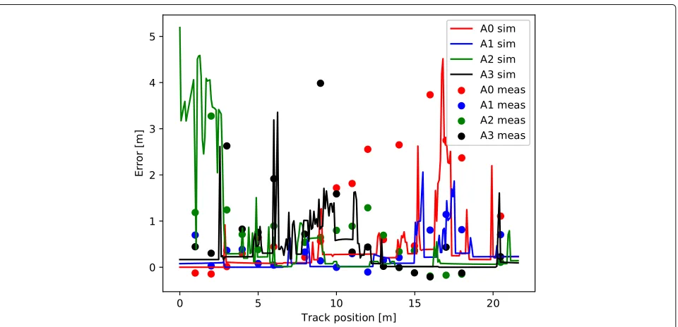
To limit the measurement time and efforts, only 18 points on a walking path were selected. On all 18 point ranges to all 4 anchor nodes were collected. The resulting ranging errors are presented as dots in Fig.4alongside the ranging errors obtained by the simulations.

Fig. 3Graphical representation of measurement probability distributions for all four anchor nodes (A0 to A3). The origin of track position is the closest point to A0

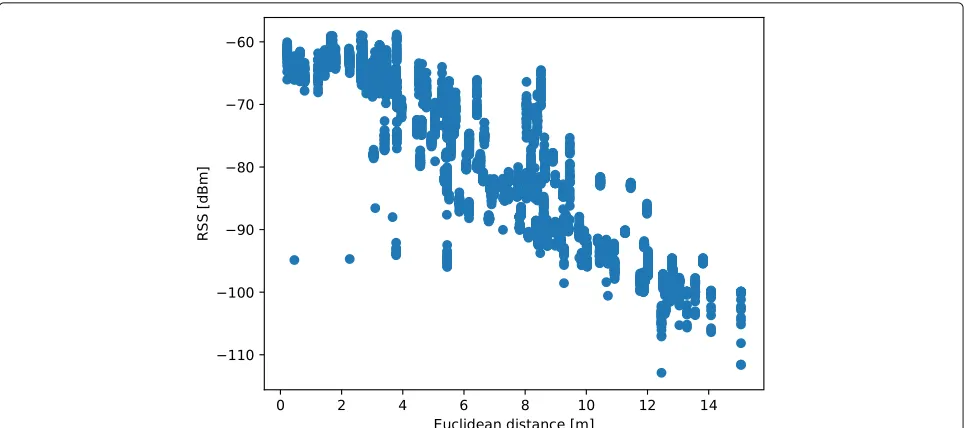
environment measurements, the shortest path signal can already be too weak to reach the receiver’s antenna and by that only the signal from longer less obstructed paths can be detected at the receiver. On the other hand, the sim-ulated loss limit of 120 dB also allowed the detection of such strongly attenuated shorter signal paths.

4 Reference tracking algorithms

In order to demonstrate the proposed simulation approach, two reference tracking algorithms were selected to evaluate the impact of round-robin ranging scheme time slot sizes on a tracking performance. A simple least squares tracking algorithm is presented in Section4.1and

Fig. 5Graphical representation of measured RSSI values at different anchor distances in the reference indoor environment

a more complex tracking algorithm based on extended Kalman filter is presented in Section4.2.

4.1 Least squares localization algorithm

The simplest approach for location estimation is based on the least squares estimator. A Euclidean distance between an UWB anchor and UWB tag is defined as

di=

(xi−x)2+(yi−y)2, (3)

wheredi is the measured range between theith anchor

(xi,yi) and the tag (x,y) with a yet-unknown location.

The system can be rewritten in a matrix form

H=

⎡ ⎢ ⎢ ⎢ ⎣

−2x1 −2y1 1 −2x2 −2y2 1

..

. ... ... −2xN −2yN 1

⎤ ⎥ ⎥ ⎥

⎦ (4)

x= ⎡ ⎢ ⎢ ⎢ ⎢ ⎣

ˆ

d₁2−x2₁−y2₁

ˆ

d₂2−x2₂−y2₂

.. . ˆ

d2_N−x2_N−y2_N

⎤ ⎥ ⎥ ⎥ ⎥

⎦, (5)

which represents a predefined system of linear equations in a normal form. The location can be estimated using the LS estimator in a normal form

ˆ

θ =(HTH)−1HTx. (6)

4.2 Extended Kalman filter-based localization algorithm

The Kalman filter is the optimal filter minimizing the dif-ference between the true and the estimated states of the

system [23]. The procedure of the Kalman filter estima-tion process consists of a predicestima-tion step and an update step. During the prediction step (7), a prediction of a new system state xˆ−_k is calculated based on a mathematical kinematic model of a system in a form of a transition func-tion k, the system’s previous state xˆ+_k−1 and an input

uk−1. The covariance of the state vector propagationP−_k

is calculated using a transition function, the previous state covarianceP+_k−1, and the process noise covariance matrix

Q_k−1. The superscript(−)designates the state after pre-diction and superscript(+)designates the state after the update step.

ˆ

x−_k =k· ˆx+_k−1+k·uk−1

P−_k =k·P+_k−1·T_k +Q_k−1 (7)

In the update step8, the Kalman gainKk is first

calcu-lated using the predicted state covarianceP−_k, the mea-surement functionHk, and the measurement covariance

matrixRk. The Kalman gain controls the magnitude of

filter’s use of predicted state estimatexˆ−_k over the mea-surement vector zk. When the measurement covariance

magnitude Rk is small, measurements are accurate and

filter weighs them more than the less reliable predicted system state. The covariance updateP+_k and the system state update after measurementxˆ+_k are then calculated as shown in (8).

Kk =P−k ·HTk ·[Hk·P−k ·HTk +Rk]−1

P+_k =[I−Kk·Hk]·P−_k

ˆ

x+_k = ˆx−_k +Kk·(zk−Hk· ˆx−k)

The underlying kinematic model defines four system state parameters (x position x, yposition y, velocity in

xdirectionx˙ and velocity inydirectiony˙). The Kalman filter implementation requires the linear system model and linear measurement model [23]. The continuous velocity linear dynamic model (9) is used as a kine-matic model but the measurement model is non-linear. When any model of a system is non-linear, the extended Kalman filter (EKF) approach needs to be employed. The idea of EKF is to linearize the non-linear equations of the dynamic model and the measurement model around the current estimation point and subsequently use the linear Kalman filter algorithm on the linearized models.

The resulting state transition function of a dynamic model (9) is depicted in (10), where t is a time between two consecutive points on a walking path or a corresponding scheduling time slot length.

k =

To model the process noise, we assume that the veloc-ities (x˙,y˙) are constant. But the movement of a person is not constant because a person is not moving along a straight line. We can assume the velocity change by a con-tinuous time zero-mean white noise w(t). Because the implementation of the filter is discrete, we need a projec-tion of the continuous noise to the instanttby our process model (t). We define the continuous noise Q_c with a

whereφSis the spectral density of the white noise.

With the integration of the termQ_cT on the [ 0,t] time interval, we get the process noise matrix (12).

Q=

The measurement model is as in the LS localization algorithm defined by (3) representing the Euclidean dis-tance between the tracked object and the anchor device.

The measurement model is non-linear, and we need to linearize it by evaluating its partial derivative at the cur-rent process statexk. The linearized measurement matrix

is represented in (13)

H=

The measurement noise matrixRin our case is a matrix with dimensions 1× 4 and is assumed to be the white Gaussian process. Four measured ranges are used dur-ing the update step of the EKF filter. If the number of available anchors increases, the dimensions of the mea-surement noise matrixRand the measurement matrixH

change.

We assume that the noise for each anchor is normally distributed around the mean which enables the use of different measurement noise levels for different anchors. According to the localization measurements in the real environment, the worst case scenario (Fig. 3) measure-ment noise standard deviationσ = 2.30 cm was used in the subsequent performance evaluation, which gives the varianceσ2_{=5.29 cm}2_.

5 Results and discussion

In order to demonstrate the proposed simulation approach, we evaluated the performance of the two selected reference tracking algorithms, focusing on the impact of measurement noise and the duration of round-robin ranging procedure time slot.

Figure 6shows the actual performance of the LS and EKF tracking algorithms in comparison to the actual walking path. We can visually analyze the performance in different situations and see the effects of different parameter settings on the actual tracking performance, which is useful during the localization and tracking system development.

The LS tracking algorithm gives very poor results because it lacks the inclusion of any kind of system mation in the process of localization, where input infor-mation (measured or simulated ranges) directly affects the result. The EKF algorithm, in contrast, uses the pre-defined kinematic model and measurement noise model for actual output filtering. The kinematic model accord-ing to the defined or expected system dynamics prevents larger output fluctuations in the presence of unexpected input signal disturbances. In other words, if the filter expects that according to the kinematic model, the speed of the tracked object in single step cannot change for more than 0.1 ms−1, the output will not change much despite the current input suggesting the sudden change of 10 ms−1_.

Fig. 6The performance of LS and EKF tracking algorithms in comparison to the actual (ground truth) walking trajectory

following four evaluation cases with different combina-tions of ground truth information (i.e., actual Euclidean distance), simulated ranging and the presence of measure-ment noise:

• The actual Euclidean distance between an anchor and a tag.

• The actual Euclidean distance with added measurement noise.

• The simulated distance between an anchor and a tag.

• The simulated distance with added measurement noise.

In Fig. 7, the performance for all 8 combinations between the 2 tracking algorithms and the 4 input data options are depicted. The simulations were performed for 6 different time-slot durations: 14.28 ms, 28.56 ms, 42.84 ms, 57.12 ms, 71.4 ms, and 85.68 ms. The results indicate that the measurement noise (i.e., the measure-ment noise of sensors excluding the ranging errors caused by NLoS and multipath propagation) has no signifi-cant influence on the tracking performance. With the increasing time-slot size, we get the increased tracking error. The actual Euclidean distance is free of multi-path error, which is a major error contribution in the RF ranging. This can be seen in the cases using sim-ulated ranges (i.e., LS sim and EKF sim in Table 1) as 80 cm worse mean error for the EKF and up to twice as much for the LS algorithm compared to tracking with the Euclidean distances (i.e., LS true and EKF true in Table1).

We can also observe the performance of tracking errors for different aspects of the observed error data. With respect to the maximum error, the EKF algo-rithm performs even better. The maximum error shown

in Table 1 is up to 4.5 times lower in the EKF

experiments than the corresponding error in the LS experiments. All performance results in terms of max-imum and mean tracking errors are represented in Table1.

6 Conclusions

For the developers of tracking systems the measure-ment of all expected trajectories in real environmeasure-ments is too complex and time consuming to be done in full. As an alternative, we propose an RF ray-tracing-based simulation approach for performance evaluation of tracking algorithms using very limited number of localization measurements for the calibration and char-acterization of the measurement noise model. Although RF ray-tracing simulations are also time consum-ing, the required human involvement is significantly lower compared to the measurements. Moreover, spe-cialized measurement equipment is not needed, and the chance for the introduction of human errors is minimized.

Fig. 7The influence of the ranging slot length on the size of mean tracking errors

durations on the final tracking outcome. The errors intro-duced by the round-robin scheduling come from the fact that each position of a moving tag in a dynamic environment is estimated from ranging samples mea-sured at different points in time and space. There-fore, the round-robin scheduled TWR tracking systems are appropriate for mostly stationary or slowly moving objects, or in applications with looser tracking accuracy and precision requirements.

As part of future work, a comparison between the round-robin and some more sophisticated ranging

scheduling protocols is planned to find an efficient ranging protocol for tracking in wireless sensor net-works, especially in dense deployments with many devices present.

Other indoor localization-related problems can also be more efficiently addressed by calibrated simulations. A very important aspect of indoor localization and tracking system deployment is optimization of anchor positions and their number in a target environment. Using aug-mented simulations, the optimal and cost-efficient anchor deployment can be planed in advance.

Table 1Mean and maximum values of tracking errors obtained by the LS and EKF algorithms with simulations and measurements

Ranging slot size

14.28 ms 28.56 ms 42.84 ms 57.12 ms 71.4 ms 85.68 ms

Mean tracking error [cm] LS true 8.7 11.1 13.9 18.3 21.6 25.4

LS sim 171.6 172.8 169.1 153.8 176.2 178.0

EKF true 8.1 12.6 15.7 20.3 24.0 26.7

EKF sim 85.3 91.2 88.3 85.1 95.5 98.7

Max tracking error [cm] LS true 39.9 39.4 44.6 52.5 59.4 76.7

LS sim 1164.6 942.1 964.5 810.0 863.1 896

EKF true 28.7 37.1 43.4 52.8 55.4 57.9

Endnote

1_{Ray-tracing simulator is publicly available athttp://e6.}

ijs.si/toolsas a part of project L2-7664 which co-funded this study.

Abbreviations

5G: Fifth generation; AoA: Angle-of-arrival; CIR: Channel impulse response; DToF: Dual-time-of-flight; EKF: Extended Kalman filter; GNSS: Global navigation satellite systems; GUI: Graphical user interface; LoS: Line-of-sight; LS: Least squares; NFC: Near-field communication; NLoS: Non-line-of-sight; PDF: Probability distribution function; RF: Radio frequency; RMS: Root mean square; RSSI: Received signal strength indicator; SBR: Shooting and bouncing; TDoA: Time-difference-of-arrival; ToA: Time-of-arrival; ToF: Time-of-flight; TWR: Two-way-ranging; UWB: Ultra-wideband

Authors’ contributions

KB contributed in conceptualization, software and hardware development, investigation, methodology, simulations, result analysis, draft manuscript writing, manuscript reviewing, and editing. RN contributed in

conceptualization, RF ray-tracing simulator software development, investigation, simulations, validation, draft manuscript writing, manuscript reviewing, and editing. MM contributed in the conceptualization and positioning of the study, reviewing and editing the manuscript, and funding acquisitions. All authors read and approved the final manuscript.

Funding

This work was partly funded by the Slovenian Research Agency (Grants no. P2-0016 and L2-7664) and the European Community under the H2020 eWINE (Grant no. 688 116) and SAAM (Grant no. 769661) projects.

Availability of data and materials

The datasets used and/or analyzed during the current study are available from the corresponding author on a reasonable request.

Competing interests

The authors declare that they have no competing interests.

Received: 27 November 2018 Accepted: 7 June 2019

References

1. R.D. Taranto, S. Muppirisetty, R. Raulefs, D. Slock, T. Svensson, H. Wymeersch, Location-aware communications for 5G networks: How location information can improve scalability, latency, and robustness of 5G. IEEE Signal Proc. Mag.31(6), 102–112 (2014)

2. A. Khalajmehrabadi, N. Gatsis, D. Akopian, Modern WLAN fingerprinting indoor positioning methods and deployment challenges. IEEE Commun. Surv. Tutor.19(3), 1974–2002 (2017)

3. N. Patwari, J.N. Ash, S. Kyperountas, A.O. Hero, R.L. Moses, N.S. Correal, Locating the nodes: cooperative localization in wireless sensor networks. IEEE Signal Proc. Mag.22(4), 54–69 (2005)

4. S. Gezici, Z. Tian, G.B. Giannakis, H. Kobayashi, A.F. Molisch, H.V. Poor, Z. Sahinoglu, Localization via ultra-wideband radios: a look at positioning aspects for future sensor networks. IEEE Signal Proc. Mag.22(4), 70–84 (2005)

5. H. Ahn, W. Yu, Environmental-adaptive RSSI-based indoor localization. IEEE Trans. Autom. Sci. Eng.6(4), 626–633 (2009)

6. K. Wu, J. Xiao, Y. Yi, D. Chen, X. Luo, L.M. Ni, CSI-based indoor localization. IEEE Trans. Parallel Distrib. Syst.24(7), 1300–1309 (2013)

7. H. Shao, X. Zhang, Z. Wang, Efficient closed-form algorithms for AOA based self-localization of sensor nodes using auxiliary variables. IEEE Trans. Signal Proc.62(10), 2580–2594 (2014)

8. H. Kim, Double-sided two-way ranging algorithm to reduce ranging time. IEEE Commun. Lett.13(7), 486–488 (2009)

9. DW1000 User Manual, Version 2.11. (DecaWave, 2017).https://www. decawave.com/sites/default/files/resources/dw1000_user_manual_2.11. pdf. Accessed 1 June 2019

10. F. Ikegami, T. Takeuchi, S. Yoshida, Theoretical prediction of mean field strength for urban mobile radio. IEEE Trans. Antennas Propag.39(3), 299–302 (1991)

11. Z. Yun, M.F. Iskander, Ray tracing for radio propagation modeling: Principles and applications. IEEE Access.3, 1089–1100 (2015) 12. N. Noori, A.A. Shishegar, E. Jedari, in2006 IEEE Antennas and Propagation

Society International Symposium. A new double counting cancellation technique for three-dimensional ray launching method, (2006), pp. 2185–2188.https://doi.org/10.1109/APS.2006.1711020

13. Z. Chen, H.L. Bertoni, A. Delis, Progressive and approximate techniques in ray-tracing-based radio wave propagation prediction models. IEEE Trans. Antennas Propag.52(1), 240–251 (2004)

14. Y. Tao, H. Lin, H. Bao, GPU-based shooting and bouncing ray method for fast RCS prediction. IEEE Trans. Antennas Propag.58(2), 494–502 (2010) 15. H. Suzuki, A.S. Mohan, Ray tube tracing method for predicting indoor

channel characteristics map. Electron. Lett.33(17), 1495–1496 (1997) 16. A. Schmitz, T. Rick, T. Karolski, T. Kuhlen, L. Kobbelt, Efficient rasterization

for outdoor radio wave propagation. IEEE Trans. Vis. Comput. Graph.

17(2), 159–170 (2011)

17. J.W. McKown, R.L. Hamilton, Ray tracing as a design tool for radio networks. IEEE Netw.5(6), 27–30 (1991)

18. R. Novak, Bloom filter for double-counting avoidance in radio frequency ray tracing. IEEE Trans. Antennas Propag.67(4), 2176–2190 (2019) 19. J.B. Keller, Geometrical theory of diffraction∗. J. Opt. Soc. Am.52(2),

116–130 (1962)

20. F. Baccelli, B. Blaszczyszyn, P. Muhlethaler, An aloha protocol for multihop mobile wireless networks. IEEE Trans. Inf. Theory.52(2), 421–436 (2006) 21. J.S. Hu, K.C. Sun, C.Y. Cheng, A kinematic human-walking model for the normal-gait-speed estimation using tri-axial acceleration signals at waist location. IEEE Trans. Biomed. Eng.60(8), 2271–2279 (2013)

22. DW1000 Datasheet, Version 2.09. (Decawave, 2015).https://www. decawave.com/sites/default/files/resources/dw1000-datasheet-v2.09. pdf. Accessed 1 June 2019

23. R. Zekavat, R.M. Buehrer,Handbook of Position Location: Theory, Practice and Advances, 1st edn. (Wiley-IEEE Press, Hoboken, New Jersey, 2011)

Publisher’s Note