On the Blind Estimation of Baud-Rate
Equalizer Performance
Jo ˜ao-Batista Destro-Filho
FEELT-UFU, School of Electronic Engineering, Federal University of Uberlˆandia, Av Jo˜ao Naves de ´Avila 2121, Campus Santa Monica, 38400-902 Uberlˆandia, MG, Brazil
Email: [email protected]
Received 20 January 2002 and in revised form 10 August 2002
This paper proposes a new method for carrying out joint blind equalization and blind estimation of the bit error rate (BER) in the output of baud-rate FIR equalizers. A simple test for assessing decision errors in the output of the decision device is derived. A comparative study of several BER estimator methods is presented in terms of convergence rate and tracking capability of both static and dynamic channels. Simulations not only validate theoretical results but also point out the effectiveness of the new proposition in terms of low computational burden and accurate BER estimation. Finally, an application of the new proposition for the detection and correction of misconvergence due to local minima issues is also presented.
Keywords and phrases:bit error rate, blind estimation, equalizer performance.
1. INTRODUCTION
The universal mobile telecommunication system (UMTS) norm [1] is the major current trend in mobile communica-tions. This norm aims at establishing a global mobile system, wherein any terminal may communicate with any other ter-minal. The terminals may be located anywhere on Earth, and the terminals may also be mobile or not. At the same time, the deployment of UMTS requires interconnection of several different local telecommunication systems in order to pro-vide the link between the two terminals. Of course, satellite communications play an important role in UMTS since they provide cost-effective international links [2, 3].
Three major characteristics of the UMTS are discussed in the following [4].
(C1) Transmission rates currently present an increasingly growing demand [1].
(C2) The communication channel is a time-variant system of difficult characterization. In fact, temporal vari-ations may be predicted with limited accuracy, and models are quite dependent both on the spatial or time scale [1]. In consequence, synchronization between the two communicating terminals is quite problem-atic due to severe fades, which requires special tech-niques for assuring the system performance, for exam-ple, adaptive transmission [5].
(C3) The management of a global communication system as UMTS is quite complex since it may be divided in
several local subsystems. Recent work [6] pointed out that, for assuring competitive quality, reliability, and availability, UMTS wireless fault management should employ an overlay system that continuously evaluates the signal quality at the level of local subsystems. For instance, [6] proposes a monitoring system based on the estimation of the bit error rate (BER).
2. ADAPTIVE EQUALIZATION AND BUSSGANG ALGORITHMS
This work focuses on blind equalization [7, 8]. In this case, the equalizer update is carried out by means of an algorithm which does not require the use of an exact copy of the trans-mitted signal. The following reasons motivate this choice.
(R1) Blind techniques may enhance the transmission rates since they do not require a training period of the equalizer.
(R2) Blind techniques avoid the accurate synchronization between transmitter and receiver, which is a stringent requirement associated with the training period of su-pervised equalization.
focuses on Bussgang algorithms. This methodology consists of a recursive optimization procedure, which is derived based on the stochastic minimization of some cost function. This cost function is defined according to some statistical crite-rion. Bussgang algorithms present several interesting features such as simple implementation, low computational burden, and well-established theoretical results.
However, Bussgang algorithms do present drawbacks which are mainly connected to the Bussgang cost functions. In fact, it has been demonstrated in [8] that for practical purposes, at least one of the local minima of all Bussgang cost functions may be associated with a poor steady-state equalization or even no equalization at all. This means that, broadly speaking, Bussgang blind techniques cannot assure all the time that equalization will take place. In consequence, the performance of Bussgang equalizers is quite dependent on the initial values assigned to the algorithm parameters.
Of course, if Bussgang equalizers are to be used in an UMTS, then it is of paramount importance to develop meth-ods to assess the equalizer performance, for example, the es-timation of the BER in the output of the blind equalizer. Such procedure is motivated by two major reasons. Firstly, it enables to monitor, detect, and provide solutions for local minima problems associated with the problematic learning of Bussgang equalizers. Secondly, in view of UMTS charac-teristic (C3), the BER in the output of a Bussgang equalizer, which is associated with a system terminal, could be consid-ered as a kind of signal quality measure at the level of a local subsystem. As the equalizer performs joint blind equalization and blind BER estimation, it is possible then to minimize the complexity of the “Performance Manager” proposed in [6] so that signal quality monitoring is partially carried out in a local basis.
3. THEORETICAL FRAMEWORK
Consider in Figure 1 the classical mathematical model used for the analysis of adaptive equalizers, where{h(n)},{c(n)}, and{v(n)}denote, respectively, the impulsive response of the channel, the linear equalizer, and the global system (channel plus linear equalizer). Besides,
v(n)=h(n)∗c(n), (1)
where the operator “∗” is the discrete convolution. Suppose that
(H1) the communication system model is baseband; (H2) the signal-to-noise ratio (SNR) is high so that the
ad-ditive noise may be neglected;
(H3) the information signalx(n) is zero-mean, iid, andM -PAM (whereMis the number of modulation levels); (H4) the communication system is linear and stable.
Notice that, although hypothesis (H1), (H2), (H3), and (H4) are restrictive, they have been extensively used in the past [9, 10] in order to analyse adaptive equalization. Besides, (H1), (H2), and (H4) are currently used [7, 8, 11] in order to derive important results in the field of local minima analysis.
Symbol
Figure1: Communication system model.
It may be demonstrated that the output of the linear equalizer is given by
wheredis equalization delay, dist(n) is distortion or inter-symbol interference,Nis channel model length,Lis equal-izer length, and v(j) is jth coefficient of the global system {v(n)}.
The main goal of the linear equalizer is to recover the in-formation signal, so that at the output of the decision device, the “open-eye” condition is verified [11]
ˆ
where Qis the distance between two adjacent levels of the
M-ary PAM signal ande(n) is the equalization error or deci-sion error. Notice that when (4) holds, the intersymbol inter-ference dist(n) may be different from zero but the output of the decision device is equal to the transmitted signal. In con-sequence, no decision error has occurred (e(n) = 0). Con-versely, if (4) does not hold, then a decision error has taken place (e(n)=1).
In the literature, (4) and (5) are rarely investigated. Most articles emphasize the following condition [12], which states that equalization is perfect as the intersymbol interference (3) is zero,
y(n)=x(n−d), (6)
dist(n)=0. (7)
Equations (6) and (7) are known in the literature as the “zero-forcing (ZF) condition.”
4. PREVIOUS WORK
equalizers. In [13], the authors propose a binary hypothesis test in order to detect errors due to an incorrect decision of the equalizer. Although such technique is quite effective and general, since it may be applied to both FIR and DFE equal-izers, it presents high computational complexity and it does not work “on-line.” In [14], the authors estimate the BER at the equalizer output by means of a neural network which computes the probability of wrong decisions. Although this method may be applied to nonlinear channels, the authors did not discuss the transient performance of the BER esti-mates which may be influenced by local minima problems connected with neural network learning.
In the most recent work of the author [15], a simple re-cursive method is developed in order to estimate the BER at the output of an adaptive equalizer. Such method is based on the blind identification of the channel by means of a high-order statistics (HOS) method followed by a simple check procedure, which recognizes whether equalization rors have taken place or not. The concept of “equalization er-ror” is considered similar to “decision error,” that is, when the output of the decision device of the equalizer is different from the transmitted signal. This simple check procedure has been derived based on the “open-eye condition” [8], which may be considered as an alternative theoretical framework with re-spect to the classical “zero-forcing” condition. The main idea behind this check is based on the following reasoning: by es-timating the channel model, we may use it along with the equalizer coefficients in order to establish whether the eye is open or not. If the eye is open, then there is no decision error. Otherwise, an estimator of the BER is updated.
Although simulation results in [15] point out that the new technique provides a BER estimator of simple imple-mentation as well as a low computational burden (with re-spect to the previous methods reported in [13, 14]), the new method does present drawbacks. Since estimation of cumu-lants is a time-consuming task, subject to error-propagation effects, the convergence of the technique proposed in [15] is slow and the absolute computational burden is still very high. These drawbacks point out that the technique may not be suitable for coping with the time variations of the mobile channel.
5. BASIC RESULTS FOR ANALYSING THE OPEN-EYE AND REVIEW OF THE PREVIOUS METHOD
Since the distortion (3) is a function of the global system co-efficientsv(j) and since each coefficientv(j) is bounded due to the stable character of {v(n)}, we may define an upper bound for the distortion dist(n) which will be represented by the symbol Sup{dist(n)}. (The operator Sup{(·)}represents the maximum value of (·)).
Suppose that
(H5) the bound Sup{dist(n)} is derived by assuming the worst case, that is, the distortion is maximum; (H6) the bound is defined by taking into account just
the effects of the transmitted signal x(n) so that Sup{dist(n)}is a function of{v(n)}.
Hypotheses (H5) and (H6) define a particular bound of the distortion, and they were proposed in [11, 16] in order to analyse the open-eye condition (4) and (5). In both arti-cles, the authors study the worst case of maximum distortion, which enables to cope with the general situation wherein the distortion may take any value lower than Sup{dist(n)}. This reasoning justifies the use of (H5) and (H6).
In [15], the author demonstrated the following theorem.
Theorem 1 (see [15]). Suppose that (H1)–(H6) hold. Then, v(d)>(M−1)·(N+L−2)·Sup
j, j=d
v(j)
=⇒x(n−d)=xˆ(n)=⇒eˆ(n)=⇒e(n)=0,
(8)
v(d)≤(M−1)·(N+L−2)·Sup j, j=d
v(j)
=⇒x(n−d)=xˆ(n)=⇒eˆ(n)=1,
(9)
where Supj, j=d{|v(j)|} (j = 0,1, . . . , N + L − 2;j = d) is the maximum absolute value of the set of coefficients {v(0), v(1), . . . , v(d−1), v(d+ 1), . . . , v(N+L−2)}andeˆ(n) is the estimation of the decision error.
Based on Theorem 1, the author proposed in [15] the fol-lowing simple recursive procedure in order to estimate the BER at the output of an adaptive equalizer (ndenotes the it-eration number). Notice that such method may be applied on-line whereas the existing estimators of the literature are not well suited for the recursive operation of the adaptive equalizer.
Procedure1 (see [15]). Givend,L,M, andNforn=1 to the total number of iterations, we
step 1: equalize the input signal and calculate the recov-ered signal ˆx(n);
step 2: estimate the channel model{hˆ(n)}; step 3: estimate the global system
ˆ
v(n)=hˆ(n)∗c(n); (10)
step 4: from{ˆv(n)}, select|ˆv(d)|and Supj, j=d{|vˆ(j)|}; step 5: compare|vˆ(d)| with Supj, j=d{|vˆ(j)|}according to (8) and (9) and calculate ˆe(n);
step 6: update the following estimator of the BER (ex-pressed in percentage):
BER(n)= n−1
n
·BER(n−1) + 100
n
·eˆ2(n). (11)
due to error propagation. This explains some limitations of Procedure 1 [15].
6. NEW THEORETICAL RESULTS FOR THE OPEN-EYE CONDITION
The following theorem, which is demonstrated in the ap-pendix, establishes further relations between the equalizer coefficients and the open-eye condition.
Theorem 2 (main result). Suppose that (H1)–(H6) hold. Be-sides, suppose that0< d < L−1. LabelSupm{|h(m)|}(m= 1, . . . , N−1)as the maximum absolute value of the set of coeffi-cients{|h(1)|,|h(2)|, . . . ,|h(N−1)|}. DefineSupq{|c(q)|}as the maximum absolute value of the set of filter coefficientsc(q) whereq=0,1, . . . , L−1andq=d. Then,
ifc(d)> B· Sup q
c(q)
=⇒x(n−d)=xˆ(n)
=⇒eˆ(n)=e(n)=0, q=0,1, . . . , L−1, q=d,
(12)
ifc(d)≤B· Sup k, k=d
c(k)
=⇒x(n−d)=xˆ(n)
=⇒eˆ(n)=1, q=0,1, . . . , L−1, q=d,
(13)
whereBis a real constant depending on the channel model
B= S
S−Supmh(m),
S= N−1
k=0
h(k). (14)
Notice that hypothesis 0< d < L−1 is a common prac-tice in the equalization literature [7, 8]. In the following, we discuss the validation of Theorem 2 in the context of an ap-plication.
7. A NEW PROPOSITION FOR CARRYING OUT JOINT BLIND EQUALIZATION AND BLIND BER
ESTIMATION
Based on Procedure 1, Theorem 2 may be used to propose an alternative method.
Procedure 2. Givend,L,M, andN forn = 1 to the total number of iterations, we
step 1: equalize the input signal and calculate the recov-ered signal ˆx(n);
step 2: estimate the channel model{hˆ(n)}by means of the “C(Q, k)” algorithm [17];
step 3: from{hˆ(n)}, select Supm{|h(m)|}and calculateB
according to (14);
step 4: compare|c(d)|withB·(Supk, k=d{|c(k)|}) accord-ing to (12) and (13) and calculate ˆe(n);
step 5: update the following estimator of the BER (ex-pressed in percentage):
BER(n)= n−1
n
·BER(n−1) + 100
n
·eˆ2(n). (15)
Notice that, in Procedure 2, the method avoids the con-volution associated with step 3 of Procedure 1, thus decreas-ing the error-propagation effects due to nonideal cumulant estimation. In consequence, Procedure 2 presents a lower computational burden and may lead to more accurate BER estimation with respect to Procedure 1. The blind estimation of the channel could be carried out by any HOS method, for example, the “C(Q, k)” algorithm [17]. This technique is chosen due to its low computational burden. The estimation of the delay d should consider the truncatedZ-transform of the inverse system C(z). However, experimental results pointed out that considering d as the half of the equalizer length, according to the center-spike initialization method [8], leads to reasonable results for any linear channel model. It should be stressed that the performance of Procedure 2 is dependent both on the HOS channel estimator as well as on the estimation of the equalization delayd. However, these issues will not be addressed in this paper. In consequence, it must be kept in mind that the performances of both Proce-dures 1 and 2 are subject to problems associated with channel model under/overestimation [18, 19], as well as with the es-timation of the delayd.
8. SIMULATIONS AND RESULTS
8.1. General description and performance criteria
A comparison among Procedures 1 and 2, the neural network described in [14], and the classical BER estimator, was car-ried out. These four estimators are, respectively, labelled as P1, P2, NN, and SP. The last one (classical estimator) is de-fined as the average of decision errors obtained by comparing the pilot signalx(n) to the recovered signal ˆx(n) according to (5). A linear filter ofL=33 taps has been used as equalizer in all simulations along with the Sato algorithm [7], whereas the radial-basis function network of method SP has 13 cen-ters in all situations.
The transmitted signalx(n) isM-PAM. All simulations and results presented are the average result of three situations
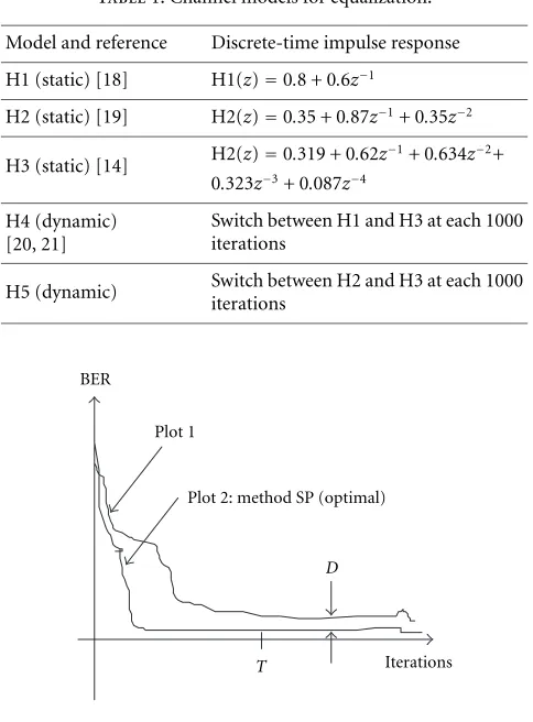
M = 2, 4, and 8. Channel models are presented in Table 1. Model H1 has been used in [20] for assessing the viability of video signal transmission through satellite according to the European DVB (digital video broadcasting) norm, whereas model H2 is nonminimum phase and is a standard model for the simulation of neural network blind equalizers [21]. H3 has been used in [14] for testing the neural network which implements method NN. Models H4 and H5 emulate a mo-bile channel [22, 23] which switches periodically between models H1/H2 and H3 at each 1000 iterations.
Table1: Channel models for equalization. Model and reference Discrete-time impulse response H1 (static) [18] H1(z)=0.8 + 0.6z−1
H2 (static) [19] H2(z)=0.35 + 0.87z−1+ 0.35z−2 H3 (static) [14] H2(z)=0.319 + 0.62z
−1+ 0.634z−2+
0.323z−3+ 0.087z−4 H4 (dynamic)
[20, 21]
Switch between H1 and H3 at each 1000 iterations
H5 (dynamic) Switch between H2 and H3 at each 1000 iterations
Iterations T
D Plot 2: method SP (optimal) Plot 1
BER
Figure2: Performance criteria.
achieve the same steady-state BER as fast as possible. Exten-sive simulation of several channel models, modulation types, and considering several SNRs pointed out that equalization takes place as the steady-state BER is lower than 5%. Besides, all results are the average among 60 Monte Carlo runs.
Figure 2 presents the convergence of the BER estimators and defines the three criteria used for assessing the perfor-mance of the methods. Notice that classical estimator SP is supposed to establish the “optimal” performance of all tech-niques since it provides the exact calculation of the decision errors. The first criterion is the convergence timeT, which corresponds to the number of iterations in order that the es-timator attains its steady-state value. The second criterion is the difference (D) between the steady-state value of the estimated BER and the steady-state amplitude of the clas-sical BER estimator (method SP). The third criterion is the quadratic error (QE), which evaluates the average quadratic difference between the value of the classical BER estimator and the amplitude of the other BER estimators considering all iterations of the convergence procedure. In Figure 2, QE is calculated by averaging the quadratic difference between all values of plot 1 (considering all iterations) and the respec-tive values of plot 2 (considering all iterations). Hence, QE characterizes the tracking capability of any BER estimation method. A low value of QE means that the method closely follows the optimal SP estimator throughout the iterations.
Table2: Results for channel H1.
Criteria SNR (dB) SP (optimal) P1 P2 NN Convergence
timeT
(iterations)
40 1000 1500 1200 1100
20 1500 2100 1800 2000
15 1657 3000 2100 2780
10 2000 6000 2500 5000
Quadratic error QE (nondimen-sional)
40 — 400 180 170
20 — 500 200 210
15 — 600 320 450
10 — 678 500 700
DifferenceD
(%)
40 — 20 5 15
20 — 27 6 20
15 — 29 10 26
10 — 30 30 40
Table3: Results for channel H2.
Criteria SNR (dB) SP (optimal) P1 P2 NN Convergence
timeT
(iterations)
40 1100 1610 1210 1200
20 1600 2160 1550 2300
15 1800 4000 2000 5000
10 2300 6800 3000 7000
Quadratic error QE (nondimen-sional)
40 — 500 190 182
20 — 600 250 250
15 — 700 345 475
10 — 750 620 900
DifferenceD
(%)
40 — 21 6 10
20 — 29 8 25
15 — 30 13 33
10 — 33 35 44
Notice that criteria convergence time (T) and QE charac-terize the transient performance of BER estimators, whereas the difference (D) characterizes the steady-state perfor-mance.
8.2. Static channels
Tables 2, 3, and 4 present the results, wherein the step size of all methods was kept constant during the adaptation. Careful analysis of Tables 2, 3, and 4 points out that
(a) concerning convergence (criterion T), P1 presents a slow convergence, whereas NN is disturbed by noise; (b) concerning tracking capability (criterion QE), the
neu-ral network NN and P2 closely follow the optimal es-timator for high SNR values. For low SNR scenarios, all methods fail; however, P2 performance seems to be robust with respect to SNR;
Table4: Results for channel H3.
Criteria SNR (dB) SP (optimal) P1 P2 NN Convergence
timeT
(iterations)
40 1200 1700 1210 1200
20 1300 2200 1400 2300
15 2000 5000 1700 6400
10 2600 7200 5000 8000
Quadratic error QE (nondimen-sional)
40 — 600 200 190
20 — 700 300 350
15 — 800 370 500
10 — 978 700 1200
DifferenceD
(%)
40 — 23 7 9
20 — 30 9 33
15 — 32 15 40
10 — 35 39 57
In brief, among the three estimators P1, P2, and NN, the neural network and the method proposed in this paper present approximately the same performance, and they are able to track the optimal estimator SP. Considering the low SNR scenario of 10 dB, procedure P2 presents the best per-formance.
8.3. Dynamic channels
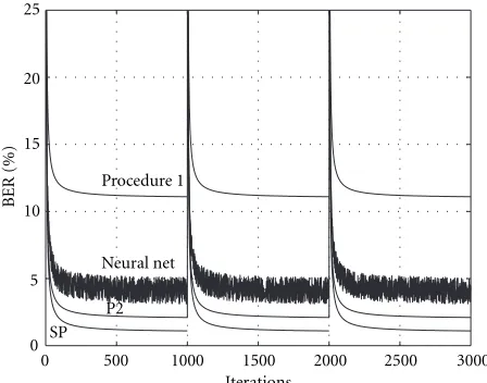
Figure 3 depicts the performance of the several estimators in the case of the dynamic channel H4 for SNR=30 dB. Proce-dure P2 and the neural network are able to track the optimal estimator closely, whereas procedure P1 cannot manage this channel. In this subsection, all algorithms were accelerated by means of adaptive step sizes. In the beginning of the adap-tation, the amplitude of the step size is set to a high value, which is progressively decreased as learning takes place. The rate of step-size amplitude reduction is controlled by diff er-ent laws, for example, exponer-ential decrease or linear decrease [7].
Tables 5 and 6 summarize the results. The conclusions from Tables 5 and 6 are the same as for the last subsection.
8.4. Computational requirements
Table 7 presents the computational burden for the several methods in terms of real additions and real multiplications per iteration, which also includes the filtering operations as-sociated with equalization (filtering of the incoming signal
u(n) and coefficients update). Special operations such as the hyperbolic tangent of the neural network as well as the se-lection process of step 3 of Procedure 2 are not considered. Clearly, procedure P2 presents a reasonable computational requirement, with respect to both the optimal SP and the neural network.
Table 8 presents the computational burden in terms of the average number of variables in memory for each tech-nique. This quantity is associated with microprocessor data memory and represents the total number of scalar quantities which must be in memory in order to perform one iteration
3000 2500 2000 1500 1000 500
0
Iterations 0
5 10 15 20 25
BER
(%)
SP P2 Neural net Procedure 1
Figure3: Equalization of the dynamic channel H4, SNR=30 dB.
Yaxis: BER (%).
Table5: Results for channel H4.
Criteria SNR (dB) SP (optimal) P1 P2 NN Convergence
timeT
(iterations)
40 400 650 450 500
20 500 700 600 650
15 600 900 630 820
10 700 990 870 870
Quadratic error QE (nondimen-sional)
40 — 500 210 200
20 — 600 250 310
15 — 720 350 500
10 — 800 800 950
DifferenceD
(%)
40 — 21 6 12
20 — 44 8 25
15 — 45 11 40
10 — 50 30 60
of the algorithm. Results are quite similar as discussed in the last paragraph.
It should be noticed that both Tables 7 and 8 were es-timated for signal processors working in a serial mode (no parallel processing).
9. APPLICATION TO LOCAL MINIMA PROBLEMS
9.1. Presentation of the problem and management
policy
Table6: Results for channel H5.
Criteria SNR (dB) SP (optimal) P1 P2 NN Convergence
timeT
(iterations)
40 455 710 460 600
20 600 850 700 730
15 700 950 710 850
10 930 990 900 900
Quadratic error QE (nondimen-sional)
40 — 570 290 250
20 — 710 300 500
15 — 900 420 1100
10 — 1200 900 1500
DifferenceD
(%)
40 — 23 7 13
20 — 50 9 33
15 — 57 13 47
10 — 60 41 71
Table7: Computational burden per iteration. Method Realadditions Realmultiplications
Classical (SP) 35 37
Procedure P1 140 156
Procedure P2 90 102
Neural network (NN) 1400 1414
not enable a reasonable signal reconstruction quality, or even no equalization at all, if the microprocessor routine does not consider the influence of SEU. This subject is developed fur-ther in the following.
Now, consider that the microprocessor implementing the Bussgang equalizer undergoes a SEU due to a solar flare event such that the value of one bit located at a place in the mem-ory unit is changed. This SEU will influence the filter adap-tation, and this effect could be modelled as a random slight deviation imposed on the algorithm variables [26]. In [27], these effects were analysed in detail, and it was pointed out that the worst impact on the system performance takes place as the SEU modifies C(n) by a random slight deviation of amplitude∆C(n),
C(n+ 1)=C(n) +∆C(n)+µe(n)·U(n), (16)
where C(n) denotes the vector containing the filter coeffi -cients at iterationn,µdenotes the step size,e(n) denotes the Bussgang error, andU(n) denotes the vector containing the signal at the input of the equalizer at iterationn.
It should be stressed that (16) is a kind of mathematical representation of the physical process leading to the change-ment of bits in some registers (or in some part of the RAM) of the microprocessor employed in the satellite receiver. Notice that the SEU may change a different number of memory bits each time that is called “severe upset” according to [25, 26].
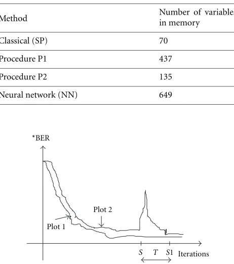
Table8: Number of variables in memory per iteration.
Method Number of variablesin memory
Classical (SP) 70
Procedure P1 437
Procedure P2 135
Neural network (NN) 649
Iterations S1
T S Plot 2 Plot 1
∗BER
Figure4: BER plots of blind equalizers. Plot 1 Standard; Plot 2 SEU effect.
Notice also that the vectorC(n) has lengthLwhere 32< L <
264 for practical purposes [7]. In consequence, the worst im-pact of a SEU on the Bussgang algorithm may lead to a bit impairment so that
32< B <264, (17)
whereBis the number of filter coefficients influenced at the same time by the SEU which is associated with∆C(n).
Figure 4 depicts two BER plots of a Bussgang equalizer. Plot 1 is associated with a standard transient behaviour, where the BER departs from a high value and gradually de-creases to a very low magnitude in the steady state. However, plot 2 illustrates the effect of a SEU, as discussed in [27]. If, by any reason, the SEU takes place at timen=S, then the BER suddenly presents a jump, increasing with high derivative in a very short period of time. Then, as the algorithms runs, the BER decreases again until the steady state is reached at time
S1 (Figure 4). The time periodT =S1−Sis called “recov-ery time” which corresponds to the time for the equalizer to overcome the SEU effect.
Table9: General procedure for the management of SEU effects on Bussgang blind equalizers.
For each iterationnof the adaptive algorithm # Estimate the BER(n)
# Estimate the BER derivative as follows:
D=BER(n)−BER(n−1) # If BER(n)>50% and ifD >50% then=> C(n+ 1)=0 0 0 · · · 1 · · · 0 0 0T
Clearly, based on the previous discussions, a simple way to detect the SEU effect would be monitoring the BER am-plitude and checking its time derivative. Then, if this deriva-tive is higher than a fixed bound, we could take an action to overcome the SEU effect. This countermeasure could be forc-ing the blind algorithm to restart adaptation, beginnforc-ing with the optimal center-spike procedure [8]. Table 9 summarizes these guidelines.
In Table 9, the bound 50% forDwas established, based on the experimental results presented in [27]. Notice that this strategy enables to cope with SEU by means of an auxiliary routine running on the microprocessor without any kind of special microelectronic hardening technique.
9.2. Results and discussion
All simulations regarding the strategy of Table 9 were carried out in a similar way as described in Section 8.1; however, just models H1 and H2 were considered. Tables 10 and 11 present results obtained for several situations. For each situ-ation (one channel model and one SNR), the following pro-cedure was employed. First, the optimal convergence of the algorithm was established, supposing the center-spike initial-ization [8]. As the algorithm achieves the steady state, the vectorC(n) is impaired so that a quantity ofBfilter coeffi -cients undergo an SEU. Then, the recovery time “T” is eval-uated as well as the steady-state BER (SS-BER).
The procedure discussed in the last paragraph was re-peated at least 100 times for each situation. Each time cor-responds to a different choice of the group ofBfilter coef-ficients which undergo the SEU effect. All results of Tables 10 and 11 were calculated by taking the average among these 100 runs.
The results of Tables 10 and 11 may be summarized as follows.
(a) Recovery times and SS-BER associated with channel 2 are always higher than their respective counterparts as-sociated with channel 1.
(b) The recovery time and the SS-BER increase as B in-creases.
(c) ForB < 10,T and SS-BER increase as the SNR de-creases. Conversely, forB >10,Tand SS-BER increase as the SNR increases. The last conclusion means that, when an extreme SEU effect takes place, additive noise contributes to the system to quickly overcome the SEU impact. This is, to some extent, a surprising result.
Table 10: Recovery timeT (iterations·103) as a function ofB (number of filter coefficients impaired by the SEU).
B Channel H1 Channel H2
40 dB 20 dB 40 dB 20 dB
1 14 16 15 22
2 15 17 16 25
3 16 20 19 27
4 19 20 20 30
5 20 23 27 31
6 21 26 29 34
7 21 29 30 34
10 32 30 37 35
15 37 30 40 38
20 39 30 43 38
25 40 30 45 40
30 43 38 50 45
33 45 43 55 47
It should be noticed from Table 11 that forB > 10, the application of the new BER estimator to channel H2 does not always lead the equalizer to a reasonable performance since the SS-BER must be equal or less than 5% in order to characterize perfect equalization. Such drawback of the SEU management proposition points out some limitations, which suggest that the “center-spike” initialization procedure [8] is not always the best strategy for all channel models.
10. CONCLUSIONS
Table11: Steady-state BER (%) as a function ofB.
B Channel H1 Channel H2
40 dB 20 dB 40 dB 20 dB
with over/underestimation of the channel model order, as well as the issue on the equalization delay estimation, are also currently under study.
APPENDIX
DEMONSTRATION OF THEOREM 2
Due to space limitations, just a sketched version of the demonstration is presented. The main background for the following analysis may be found in references [28, 29]. The demonstration is divided into three steps. In the first one, an expression for the maximum absolute value of coefficient
v(n) (wheren=0,1,2, . . . , N+L−2 andn=d) is derived, whereas in the second step, an expression for the minimum absolute value of coefficientv(d) is derived. In the third step, the previous results are used to demonstrate (12). Demon-stration of (13) is not provided since it follows a similar pro-cedure as for (12).
Step (1): The maximum absolute value of coefficientv(n) (wheren=d)
According to (1) and the definition of discrete convolution, the coefficientv(n) may be expressed as
Then, applying the triangle inequality to the module of (A.1), we have
Bounds forS1 andS2 are now established. Suppose that 0< d < L−1 which is a common practice in the equalization literature [7]. Beginning with (A.3) and taking into account thatn =0,1, . . . , N +L−2,n =d, then we conclude that
Turning toS2, notice that the main goal of the theorem is to analyse the mathematical relationship between coefficient
c(d) and the other coefficientsc(k), wherek=0,1, . . . , L−1 andk = d. Label the maximum absolute value of all coef-ficientsc(k) as Supq{|c(q)|}, whereq = 0,1, . . . , L−1 and
q=d. Since Supq{|c(q)|}is a constant for anyqandk, the following inequality presents a bound for sumS2:
S2≤Sup Then, comparing (A.6) and (A.9) to (A.2), it is possible to conclude that Notice that the choice of the maximum absolute value is not unique. The works [26, 27] study an inequality closely related to the expression (A.10). One possible maximum is obtained by considering the equality signal in (A.10), which is validated by the information theory calculations in [27]. So, the following maximum is chosen:
Supv(n)=c(d)·Sup
Step (2): The minimum absolute value of coefficientv(d) The constantbis now defined as
b=(M−1)·(N+L−2), (A.12)
where M is the number of modulation levels of the signal
x(n),N is the channel model length, andLis the equalizer length.
Since, in practice,Mmay take the values{2,4,8,16,32,
64,128,256}, then
M−1≥1. (A.13)
In practice [7], it is common to use an equalizer length which is higher than the channel length
1≤N < L, L≥2=⇒(N+L−2)≥1. (A.14)
So, combining (A.13) and (A.14), the integerbin (A.11) obeys the following inequality:
Now consider the sum in the right side of (A.16). Com-bining (A.4) and (A.7), supposing in this case thatn=d, it is possible to state that
In the right side of inequality (A.17), the summation may involve all terms|h(k)|,k=1,2, . . . , N−1,k=0. Then we
Since the constantbis an integer greater than or equal to 1 according to (A.15) and based on (A.18), we may conclude that
Comparison between (A.16) and (A.19) leads to the fol-lowing inequality From the previous inequality, notice that
Infv(d)≤v(d)
where Inf{|v(d)|}represents the minimum absolute value of
v(d). Based on (A.21), it is possible to choose the minimum absolute value of coefficientv(d) as
Infv(d)=b·c(d)· N−1
k=0
Again, we may argue that this is not the unique choice for the minimum value. This issue is discussed in detail in refer-ences [28, 29] which provide theoretical basis for the choice in (A.22).
Step (3): Final demonstration
It is supposed that the following condition holds by hypoth-esis:
c(d)> B·Sup q
c(d), q=0, . . . , L−1, q=d,
(A.23)
B= S
S−Supmh(m), m=1,2, . . . , N−1, (A.24)
S= N−1
k=0
h(k). (A.25)
Replacing (A.24) into (A.23) and reordering terms of the inequality, we may get
S·c(d)>c(d)·Sup m
h(m)+S·Sup q
c(q). (A.26)
Since the constantb is an integer greater than or equal to 1 according to (A.15), then we may multiply both sides of (A.26) bybwithout changing the sign of the inequality
b·S·c(d)> b· c(d)·Sup m
h(m)+S·Sup q
c(q).
(A.27) We recognize that the right side of (A.27) is exactly the maximum absolute value of (A.11) and that the left side of (A.27) is exactly the minimum absolute value of (A.22). In-serting (A.11), (A.12), and (A.22) into (A.27), we get
Infv(d)>(M−1)·(N+L−2)·Supv(n). (A.28)
Notice that
v(d)>Infv(d). (A.29)
From (A.29) and (A.28), we may write
v(d)>(M−1)·(N+L−2)·Supv(n). (A.30)
Finally, using (8) of Theorem 1, we may conclude from (A.30) that the eye is open. This completes the demonstra-tion.
ACKNOWLEDGMENTS
The author thanks CNPq, Fapesp, and CAPES for the finan-cial support of this work, as well as Prof. Caio J. C. Negreiros (Institute of Mathematics/Unicamp) for insightful discus-sions. Special thanks are also addressed to the anonymous reviewers, as well as to Dr. R. Pirjola (FMI-Finland) and Dr. E. de Paula (INPE-Brazil) for discussions and references on radiation effects on satellite communications.
REFERENCES
[1] J.-C. Bic, A. Charbonnier, D. Duponteil, N. Ruelle, S. Tabbane, and J.-P. Taisant, “Radiocommunications and mobility,”Ann. T´el´ecommun., vol. 50, no. 1, pp. 114–141, 1995.
[2] Special Issue on Global Positioning System,Proceedings of the IEEE, vol. 87, no. 1, January 1999.
[3] http://www.cost280.rl.ac.uk.
[4] R. D. Yates and N. B. Mandayam, “Challenges in low-cost wireless data transmission,”IEEE Signal Processing Magazine, vol. 17, no. 3, pp. 93–102, 2000.
[5] A. Duel-Hallen, S. Hu, and H. Hallen, “Long-range prediction of fading signals,” IEEE Signal Processing Magazine, vol. 17, no. 3, pp. 62–75, 2000.
[6] J. Vucetic, P. Kline, and J. Plaschke, “Implementation and per-formance analysis of multi-algorithm dynamic channel allo-cation in a wideband cellular network,” inProc. IEEE/ICC ’96 Conference, pp. 1270–1274, Dallas, Tex, USA, June 1996.
[7] S. Haykin, Ed.,Unsupervised Adaptive Filtering, vol. 1-2, John Wiley and Sons, New York, NY, USA, 2000.
[8] Z. Ding and Y. Li,Blind Equalization and Identification, Mar-cel Dekker, New York, NY, USA, 2000.
[9] A. Benveniste and M. Goursat, “Blind equalizers,” IEEE Trans. Communications, vol. 32, no. 8, pp. 871–883, 1984. [10] O. Shalvi and E. Weinstein, “New criteria for blind
decon-volution of nonminimum phase systems (channels),” IEEE Transactions on Information Theory, vol. 36, no. 2, pp. 312– 321, 1990.
[11] Z. Ding, C. R. Johnson Jr., and R. A. Kennedy, “Global con-vergence issues with linear blind adaptive equalizers,” inBlind Deconvolution, S. Haykin, Ed., pp. 60–120, Prentice-Hall, En-glewood Cliffs, NJ, USA, 1994.
[12] J. G. Proakis, Digital Communications, McGraw-Hill, New York, NY, USA, 3rd edition, 1995.
[13] K. Doganc¸ay and R. A. Kennedy, “Blind detection of equal-ization errors in communication systems,”IEEE Transactions on Information Theory, vol. 43, no. 2, pp. 469–482, 1997. [14] J. Cid-Sueiro and A. R. Figueiras-Vidal, “Non-linear
equal-izers that estimate error rates during reception,” in Proc. EURASIP/EUSIPCO ’98, Rhodes, Greece, September 1998. [15] J. B. Destro Filho, J. P. Breda Destro, and J. M. Travassos
Ro-mano, “On-line evaluation of equalizer performance based on high-order statistics,” inProc. EURASIP/EUSIPCO ’2000, pp. 1521–1524, Tampere, Finland, September 2000.
[16] R. W. Lucky, “Automatic equalization for digital communi-cation,”Bell System Technical Journal, vol. 44, no. 4, pp. 547– 588, 1965.
[17] G. B. Giannakis, “Cumulants: A powerful tool in signal pro-cessing,”Proceedings of the IEEE, vol. 75, no. 9, pp. 1333–1334, 1987.
[18] B. Porat and B. Friedlander, “FIR system identification using fourth-order cumulants with application to channel equaliza-tion,”IEEE Trans. Automatic Control, vol. 38, no. 9, pp. 1394– 1398, 1993.
[19] F.-C. Zheng, S. McLaughlin, and B. Mulgrew, “Blind equaliza-tion of nonminimum phase channels: Higher order cumulant based algorithm,”IEEE Trans. Signal Processing, vol. 41, no. 2, pp. 681–691, 1993.
[20] C. S. Lee, S. Vlahoyiannatos, and L. Hanzo, “Satellite based turbo-coded, blind-equalized 4-QAM and 16-QAM digital video broadcasting,”IEEE Trans. On Broadcasting, vol. 46, no. 1, pp. 23–33, 2000.
[22] D. W. Matolak, “On the multi-state modeling of mobile satel-lite channels,” inProc. MILCOM 2000, Los Angeles, Calif, USA, October 2000.
[23] H. H. Yang and S.-I. Amari, “Blind equalization of switching channels by ICA and learning of learning rate,” inProc. IEEE Int. Conf. Acoustics, Speech, Signal Processing, vol. III, pp. 1849–1852, Munich, Germany, April 1997.
[24] H. Koskinen, E. Tanskanen, R. Pirjola, et al., “Space weather effects catalogue,” Report 2001:1, Finnish Meteorological In-stitute, Helsinki, Finland.
[25] R. Ecoffet, M. Sarthou, M. Labrun´ee, L. Gasc, and A. Dubreuil, “Space SEE risk assessment for a commercial digital TV receiver,” IEEE Trans. on Nuclear Sciences, vol. 44, no. 6, pp. 2333–2336, 1997.
[26] T. Goka, H. Matsumoto, and N. Nemoto, “SEE flight data from Japanese satellites,”IEEE Trans. on Nuclear Sciences, vol. 45, no. 6, pp. 2771–2778, 1998.
[27] J. B. Destro-Filho and D. Matolak, “Effects of solar flares on satellite communications: issues for blind equalizer design,” inProc. RADECS ’2001, Grenoble, France, September 2001. [28] M. R. Leadbetter, G. Lindgren, and H. Rootz´en, Extremes
and Related Properties of Random Sequences and Processes, Springer-Verlag, New York, NY, USA, 1983.
[29] E. Arikan, “An inequality on guessing and its application to sequential decoding,” IEEE Transactions on Information The-ory, vol. 42, no. 1, pp. 99–105, 1996.
Jo˜ao-Batista Destro-Filhowas born in S˜ao Jos´e do Rio Pardo, SP, Brazil, 1970. He received the B.S.E. degree in 1991 and the M.S. degree in 1994, both from the School of Electrical and Computer Engi-neering (FEEC), University of Campinas (Unicamp), SP, Brazil. He received the Ph.D. degree in signal processing from the I3S Laboratory-CNRS, University of Nice-Sophia Antipolis, France, in 1998. During