Model-Based Real-Time Head Tracking
Jacob Str ¨om
Multimedia Technologies Department, Ericsson Research, Torshamnsgatan 23, 164 86 Stockholm, Sweden Email: [email protected]
Received 31 August 2001 and in revised form 29 May 2002
This paper treats real-time tracking of a human head using an analysis by synthesis approach. The work is based on the Structure from Motion (SfM) algorithm from Azarbayejani and Pentland (1995). We will analyze the convergence properties of the SfM algorithm for planar objects, and extend it to handle new points. The extended algorithm is then used for head tracking. The system tracks feature points in the image using a texture mapped three-dimensional model of the head. The texture is updated adaptively so that points in the ear region can be tracked when the user’s head is rotated far, allowing out-of-plane rotation of up to 90◦without losing track. The covariance of thex- and they-coordinates are estimated and forwarded to the Kalman filter, making the tracker robust to occlusion. The system automatically detects tracking failure and reinitializes the algorithm using information gathered in the original initialization process.
Keywords and phrases:face tracking, modeling, real-time, EKF, structure from motion, planar objects, analysis by synthesis.
1. INTRODUCTION
Automatic tracking and modeling of human faces from im-age sequences is an important and challenging task in com-puter vision. Applications include face recognition, model-based coding for video conferencing, avatar control, and computer graphics. The main goal of this paper is to present a tracking system built on the extended Kalman filter based SfM algorithm in [1], thus extending the foundations of Azarbayejani and Pentland and Jebara and Pentland [2] to achieve robust performance. Since points on the face might lie in a nearly planar constellation, the stability of the SfM algorithm is investigated for planar surfaces. The theory of Triggs for SfM of planar objects will be used as a starting point, and simulations on both noise free and noisy data are carried out to investigate how often the algorithm converges. The results are compared to general three-dimensional ob-jects. The algorithm is also extended to handle new points, that is, points that are not visible in the first frame. This poses a problem since the first frame is used as a reference frame in the error function that the Kalman filter is minimizing. Three ways to handle these new points are investigated, and the re-sulting solution is to keep the old reference frame for the old points and use the new reference frame for the new ones.
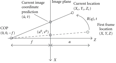
The results will be applied to a face tracking system. The core idea is to select a dense set of feature points (es-sentially, optical flow at all the most information bearing points). Figure 1 illustrates how the system works. Patches around the feature points taken from the rendered three-dimensional model (lower left corner) are matched against the incoming video, and the two-dimensional trajectories
of these feature points are then fed through an extended Kalman filter (EKF) to update the pose information of the three-dimensional model. In addition, the projection of the estimated structure serves as a starting point for the tracking in the next frame. The three-dimensional model helps in sev-eral ways. First, it compensates for rotation and scale, mak-ing it possible to use fast two-dimensional block-matchmak-ing to track the feature points. Second, it helps in assessing how reliably a certain feature point can be tracked. For instance, a feature point depicted at a steep angle to the camera is hard to track and a feature point on the back side of the model cannot be tracked at all. The estimate of the relia-bility of a point can then be forwarded to the SfM Kalman filter as a covariance of the noise in the two-dimensional point measurements. Third, by tracking features on the side of the head, the system can cope with large out-of-plane rotations.
1.1. Previous work
Pose 3D structure
focal length 3D point model
Pose, focal length Rendered 3D surface model
Texture update
2D patch tracking
Video input New points Measurements (2D trajectories)
3D structure is used
as starting point
EKF structure from motion
Variance estimates (from 3D model
and residuals)
Figure1: Patches from the rendered image (lower left corner) are matched with the incoming video. The two-dimensional feature point trajectories are fed through the SfM extended Kalman filter that estimates the pose information needed to render the next model view. For clarity, only four patches out of 24 are shown.
local motion. Li et al. [8] extend the system of Roivainen to work directly on image gradients, without the need to calcu-late the optical flow. In a calcu-later paper, Li and Forchheimer [9] modify their algorithm to include M-estimation, which is a robust version of the least squares algorithm. DeCarlo and Metaxas [10] use a very detailed parameterized head model constructed using anthropological data. The parameters are changed using a deformable model framework, where edges in the image give rise to forces on the parameters. Cootes et al. [11] use Active Appearance Models (AAMs), where a face is modeled using a combined eigenspace for texture and shape. By learning a function from the residual error to the eigenspace parameters, the algorithm can be iterated on a face image until convergence. Cootes et al. have used their algorithm on image sequences, where the shape from the pre-vious frame is used as a starting value in the next one. Cas-cia et al. [12] use a three-dimensional version of the Active Appearance Model method. Instead of modeling the shape using a two-dimensional PCA, a cylinder model of the head is used, and an illumination eigenspace is added to the er-ror function to gain robustness. Cascia et al. reports real-time performance (15 Hz) on an SGI O2 machine. Ahlberg [13] uses the three-dimensional CANDIDE model [7] for face tracking using AAMs in real time.
The method presented in this paper is a continuation of the work by Azarbayejani and Pentland [1], Jebara and Pentland [2], and Str¨om et al. [14]. In their SfM paper [1], Azarbayejani and Pentland show a head tracking application. The feature points are obtained by normalized correlation, and the tracker resolves rotation and translation of the head as well as point depths and focal length. Jebara and Pentland [2] extend the work to a real-time system, and use the es-timated three-dimensional structure as a starting point for the normalized correlation in the next frame. This greatly enhances the robustness since an incorrectly tracked feature point can be corrected by the other points, so that its start-ing position in the next frame will be reasonable. Jebara and
Pentland also estimate the covariance of the noise in the mea-sured point positions from the residual error, which gives robustness to partial occlusion. Furthermore, each point is tracked for rotation and scale, doubling the degrees of free-dom in the measurements. The work by Str¨om et al. [14] adds a three-dimensional head model, which is useful for (a) projectively transforming all templates that are used in the normalized correlation at once, reducing the cost of adding another point, and (b) predicting when points on the face are turning away from the camera or are self occluded. This paper further extends the work in [14] by incrementally up-dating the texture to track points on the side of the head. In this manner, the head can rotate farther before losing track.
Azarbayejani and Pentland [1] evaluate the stability of the SfM algorithm for general three-dimensional objects for different types of motion at various noise levels. No at-tempt is made to evaluate the algorithm with planar ob-jects. Indeed, this is an important special case, since points on the surface of a face can be close to planar. Furthermore, many SfM algorithms have shown to fail for planar objects [15, 16, 17]. Triggs provides a theory for how many frames are needed to solve the SfM problem in the planar case, and also proposes an algorithm for autocalibration [18]. Tenta-tive results on the stability of the algorithm of Azarbayejani and Pentland have been presented in [19], but only for the noise-free case. The reinitialization algorithm was first pro-posed in [20].
1.2. Overview
Section 2 will recapitulate the SfM algorithm, investigate its stability for planar surfaces and extend it to allow new points. Section 3 will go through the tracking; initialization, indi-vidual point tracking, estimation of the measurement noise covariance and texture update. Section 4 will treat how the system is reinitialized once it loses track. This is followed by a system evaluation in Section 5. The paper is concluded in Section 6.
2. KALMAN FILTER BASED SfM
Azarbayejani and Pentland reformulate the SfM problem into a stable recursive estimation problem that has been shown to converge reliably [1, 23]. A three-dimensional point is parameterized with its image coordinates in the first frame, (u0, v0), and its depthα, using
whereβis 1/focal length. This is shown in the dashed line in Figure 2. The unknown parameters constitute the state vec-torx; the rotation and translation from the first frame to the current, the inverse focal lengthβand the point depths α. To predict the image plane projection of the points in the kth frame, the function ( ˆu1,vˆ1,uˆ2,vˆ2, . . . ,uˆN,vˆN)=hk(¯x) is
used. As shown in Figure 2, the effect ofhk(¯x) is to
calcu-late (X, Y, Z) using (1) and then rotate, translate, and finally project the points using the parameters from the state vec-torxk. Ifzkis the measured image coordinates of the feature
points, the movement, the focal length, and the depths can be updated using
whereKkis the Kalman gain [24].
2.1. Planar objects
Planar objects are important for two reasons. First, man-made structures contain many planar objects such as walls, floors, desks, and so forth. Second, some objects might be close to planar. In the case of face tracking for instance, a small number of randomly picked points on the surface of the face might be close to coplanar. If the SfM algorithm fails for planar objects, it is likely to do poor on such nearly pla-nar objects. Furthermore, it is a well-known fact that plapla-nar objects constitute a singular case that many SfM algorithms have problems with. For instance, it is not possible to cal-culate the coefficients of either the bifocal [17] or the trifo-cal tensor [15] for planar objects in the untrifo-calibrated case. Stein and Shashua [16] show that problems also occur for objects made up of several planes that intersect in a sin-gle line, and also point to several real world objects that fit this description. Triggs shows that whennintrinsic camera parameters are unknown (but constant), m = (n+ 4)/2
Figure2: Using the original frame coordinates (u0, v0), the depthα
and the focal length 1/β, (X, Y, Z) is obtained. This vector is further moved to (Xc, Yc, Zc) and finally projected to the image coordinate prediction ( ˆu,v).ˆ
images are needed for uniqueness. In the uncalibrated case whenn= 5,m = (5 + 4)/2 = 5 images are thus needed for uniqueness. If fewer intrinsic camera parameters are es-timated, it should still be possible to use multilinear con-straints. If, for instance, only the (constant) focal length is unknown, m = (1 + 4)/2 = 3 images are sufficient, and the trifocal tensor could be used. However, the constraints on the remaining four intrinsic camera parameters turn into polynomial constraints on the tensor coefficients that are not easily solved.
2.2. Several views of a planar object
The EKF approach to the SfM problem does not rely on only two or three images, but instead it takes an entire sequence of images into account. Whether the filter will converge for a planar object is not obvious. On the one hand, the previous section indicates that three images are enough for unique-ness. On the other hand, the constraints of all the images are not applied simultaneously; at each time stepk, the problem will be under-determined and a manifold of false structures will be possible. To resolve this a Monte Carlo experiment is conducted. Random points are selected from a plane, which is randomly oriented. The object undergoes random motion and the point measurements are forwarded to the Kalman filter. The filter runs for 1000 frames and if the summed squared error of the estimated depth values is smaller than 0.1, convergence is declared. The experiment is repeated 1000 times using two types of motion:rotationaround a random vector in thez =0 plane (to avoid the degenerate rotation around thez-axis) andBrownian motion, that is, small incre-mental random steps in translation and rotation. The filter is initialized with β = 2.0 (the true value is β = 1.3). Three types of initialization procedures are tried for the depths α1,...,N−1: in the first type, calledprior 1, theα-values are set
to random values in the interval±0.5 around the depthα0
Table 1: Depth convergence frequency for noise free measure-ments.
prior 1 prior 2 prior 3 2D rotational 0.673 0.953 1.000 3D rotational 0.796 1.000 1.000
2D brownian 0.751 0.972 1.000
3D brownian 0.762 1.000 1.000
Table2: Depth convergence frequency for noisy measurements.
prior 1 prior 2 prior 3 2D rotational 0.656 0.898 0.987 3D rotational 0.802 0.995 1.000
2D brownian 0.508 0.851 0.924
3D brownian 0.478 0.943 0.981
is then repeated for a random three-dimensional object. This time, prior 1 will mean that all theα-values are initialized to the same value 1.0, whereas the prior 2 and prior 3 will mean that theα-values are initialized to the correct value plus ran-dom noise in the intervals±0.5 and±0.25, respectively. The result is shown in Table 1 for the case of noise-free measure-ments.
As can be seen, there are differences between the pla-nar (2D) and the general (3D) objects, but as the quality of the depth prior improves, the convergence frequency goes to unity for both types of objects. In the case of noisy mea-surements, the difference is larger. In Table 2, uniformly dis-tributed noise of ±1 pixel is added to the measurements. Still, the difference is quantitative, not qualitative. One ex-ample is when tracking a planar object undergoing Brown-ian motion, with depth prior 3 (third row, third column). In this case, one has as much to gain by changing the mo-tion to rotamo-tional as changing the planar object to a general three-dimensional one (convergence frequency rises to 0.987 compared to 0.981). Hence, a planar object is not a catas-trophic situation that means that the SfM algorithm will un-conditionally fail. Rather, planar objects can be seen as some-thing that should be avoided if possible, just like measure-ment noise, poor depth priors, or low excitation in the mo-tion. A way to understand why the filter converges for planar views is the following. The SfM problem at imagekcan be formulated as finding the state vectorxwhich minimizes the (scalar) error function
where hk(x) consists of the Kalman filter’s estimate of the
projected points ( ˆu1,vˆ1,uˆ2,vˆ2, . . . ,uˆN,vˆN). Each new image
k gives a new constraintJk(x) = 0. Since the object is
pla-nar and since the focal length is constant (not varying over time) but its value unknown. m = (1 + 4)/2 = 3 im-ages are needed for uniqueness, but only two imim-ages are part of Jk(x). Therefore, an entire curve xk(t) of false
so-lutions will satisfy Jk(x). If this curve is projected down
Sk+1(t)
Figure3: Structure convergence for planar objects.
1000
Number of iterations before convergence 0
Number of iterations before convergence 0
Figure4: (a) Histogram over convergence time for rotational mo-tion with a general object (solid) and a planar object (dotted). (b) Ditto for Brownian motion.
to only the structure components of x, a new curve sk(t)
is obtained, where s = (β, α1, α2, . . . , αN). Since the
solu-tion is unique for three views, sk(t) andsk+1(t) cannot be
Z
Figure5: Expected bias in (u0
new, v0new) when the depth of the new
point (Xnew, Ynew, Znew) is unknown.
2.3. Appearing points
In a tracking scenario, it is advantageous to be able to track points that were not visible in the first image. In the exam-ple of head tracking, for examexam-ple, it is desirable to be able to track points on the ear when the head turns sideways. It is thus essential that the algorithm is able to include some of the new points that have appeared. The last part of this sec-tion will treat how points can be added to the Kalman filter based SfM algorithm. The work described here was presented in [21]. Independently, Dell’Acqua et al. [22] later published similar work. However, their solution differs from the one presented here and will be treated at the end of this section.
As described in the beginning of Section 2, the function
hk(·) uses the image coordinates in the first frame, (u0, v0), to
calculate (X, Y, Z), (XC, YC, ZC), and then the estimate ( ˆu,vˆ).
The fact that (u0, v0) must be known in order to calculate the
filter estimates poses a problem when adding feature points at a later stage. If a new feature point becomes visible first at framek, its image plane projection in the original reference frame (u0
new, v0new) is not known.
2.3.1 Old reference frame
One way to solve the problem is to rotate and translate back the measurements from thekth frame to the 0th frame. As can be seen in Figure 5, however, the lack of knowledge of the depth αwill result in a large bias in the estimation of (u0
new, vnew0 ).
2.3.2 New reference frame
Another solution would be to change the reference frame and restart the Kalman filter at the kth frame. As can be seen in Figure 6 a similar problem to that of Figure 5 oc-curs: for each old point, the image coordinates from the first frame (u0old, v0old) (solid circle) are replaced with estimates
(uk
old, vkold) in thekth frame (middle dashed circle). The depth
αis not known exactly, and this creates a bias in the position of (ukold, voldk ) (other dashed circles). Since the filter has had
some time to converge, there is an estimate ofα, and the bias
Z
Figure6: The bias in the position (uk
old, voldk ) in the new reference
frame when the depth of an old point is not known exactly (lower black interval).
Figure7: The proposed method—the old points will keep the old reference frame, whereas the new points will use the new reference frame. No bias due to depth will occur.
of (uk
old, voldk ) is thus smaller than with theold reference frame
method of Figure 5. On the other hand, bias is added toall
the old points, compared to only the new points, which are assumed to be fewer.
2.3.3 Bias estimation
Both the old reference frame and the new reference frame
methods will thus suffer from bias. One solution to this is to include this bias in the state vector and estimate it using the Kalman filter. Bias estimation was proposed in the original paper by Azarbayejani and Pentland [1], but not specifically as a solution to the problem of adding points. Equation (1) is then modified to
troducing these extra degrees of freedom will make the filter less over-determined.
2.3.4 Two reference frames
As illustrated in Figure 7, the old points will continue to be restricted to the line from the center of projection (COP) to (u0old, v0old), whereas the new points will lie on the line from
the COP to (uk
new, vnewk ). The prediction ( ˆu,vˆ) for the old
points will continue to be calculated using (the projection of) (5), whereas the new points will be calculated according to the projection of
and translation between frame 0 and framek.
This approach is still not bias free—estimation errors in the rotation quaternion and in the translation vector will give rise to a shift in the texture map and hence a bias in (uk
new, vnewk ). However, this problem also occurs with the
other methods. Moreover, in the proposed scheme the ro-tation and translation bias only applies to the new points, as opposed to all the old points in thenew reference frame
method. As mentioned above, these biases inuandvcan be estimated. Alternatively, the motion parameters RTk andTk
can be estimated. This amounts to only 6 extra degrees of freedom for the filter, which is advantageous to estimatingbu
andbvif more than 3 points are added at once. The
imple-mentation of the real system (described in Section 3), did not seem to suffer from these biases, and thetwo reference frames
method could be used without extending the feature vector for bias estimation.
2.3.5 Related work
Recently, the problem of adding points to the EKF based SfM algorithm has been investigated by Dell’Acqua et al. [22]. Their solution is to start an independent Kalman filter each time a new point occurs. After collecting data from the en-tire sequence, a single Kalman filter is stitched together from all the others. Each time a point disappears from themaster
Kalman filter, all theslavefilters that have been created up to that point are examined for replacement candidates. The point that will survive the longest is then used to replace the old point. Theold reference frame method is used, and the bias of the new point can be reduced since the depthαcan be obtained from theslaveKalman filter, that has been con-verging for a while. Themasterfilter is then continued until a new point disappears, and the procedure is repeated. No at-tempt is made to reacquire old points—when they reappear they are treated as new, unknown points.
Since the above-mentioned method is of batch type it is not well suited for real-time tracking. It can obviously be modified so that no look-ahead is used, but even so the use of multiple Kalman filters (one filter for each new point) makes it a bit computationally expensive in a real-time scenario. Furthermore, just as in thenew reference framemethod, any remaining error in the estimated depthαwill result in some bias. On the other hand, there are advantages to having all points in the same reference system. For instance, the extra
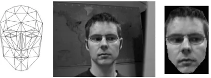
Figure 8: A generic three-dimensional polygonal head model is aligned with a head-on shot of the video sequence, and the corre-sponding pixels are texture mapped to the surface of the face model.
matrices for rotation and translation (RkandTk) of (5) are
avoided.
3. HEAD TRACKING
In this section, the extended SfM algorithm from Section 2.3.4 will be used in a head tracking application. Recalling Figure 1, the head is rendered using a generic polygonal face model1 [7] in the predicted pose (lower left). Patches from
this rendered image are matched against the incoming video (top left). The two-dimensional measurements are fed into the SfM Kalman filter that calculates the three-dimensional structure, pose and focal length for a point configuration defined by the center of each patch. The pose and the focal length are then used to render the polygonal model, and the structure is used to predict the positions of the patches’ cen-ters in the next frame. Whereas the solid arrows in Figure 1 represent information flows that occurs every frame, the dashed arrows are invoked only at texture update. When the head has turned sufficiently, texture is grabbed, and both the three-dimensional model (bottom left) and the extended Kalman filter (upper right) are updated.
3.1. Initialization
The system is initialized from a frontal position as seen in Figure 8. The face model (left) is aligned to match with a head-on view of the face in the video sequence (middle). The pixels from the video are then texture-mapped onto the model (right). Our system uses a manual alignment—the user has to put the head in a prespecified position on the screen, and make sure that she/he is in a frontal position be-fore initiating tracking.
After alignment has been performed, the system selects which feature points to use. The part of the video input con-taining the face is cropped out (first image of Figure 9) and further processed. The cropped image is lowpass filtered and subsampled once to avoid locking on to features that are too vague to be reliably tracked. The determinant of the Hessian
Ixx Ixy
IxyIy y
is calculated at every point. To avoid selecting points on parts of the face surface perpendicular to the camera, the determinant is weighted with the cosine of the angle between the surface normal and the camera direction. These values
Figure 9: From left: The lowpass filtered incoming video, the weighting (the cosine of the angle between the surface normal and the camera direction), the final rating, and the extracted feature points.
can easily be obtained from the computer graphics hardware by rendering a gray shade version of the three-dimensional model with lighting from the camera direction (Figure 9, second image). The resulting rating of each pixel is shown in the third image in Figure 9, where brighter pixels indi-cate a higher score. The 24 points with the highest ratings are then selected with a minimum-distance constraint be-tween points. The fourth image in Figure 9 shows 12 of the 24 points selected. Each point is given a three-dimensional po-sition on the surface of the three-dimensional model. Again, the computer graphics hardware can be used, this time read-ing out the value of the depth buffer of the rendered image in the corresponding pixel location, to calculate the depth of the feature point.
3.2. Feature point tracking
As shown in Figure 1, the tracking is carried out between the rendered frame and the video input. Both images are sub-sampled in order to track larger and more robust features. Since the feature points are fixed with respect to the three-dimensional model, their two-three-dimensional coordinates in the rendered image are known. A 7×7 pixel patch around each feature point is cropped out. This patch is then matched with patches from the video input image in a 17×17 pixel search window using weighted normalized correlation. More specifically, ifaandbare the vectors obtained by raster scan-ning the patch in the rendered image and the video input respectively, then the ˆbthat maximizes
=G(x, y) cos(θ)=G(x, y)aˆ·bˆ ˆ
abˆ (6)
is selected, where ˆa=a−µa, ˆb=b−µb, · represents the norm, andG(x, y) is a Gaussian weighting function that pun-ishes large jumps of the patches. The search window is cen-tered around the position that is estimated from the structure from motion algorithm. An exhaustive search is carried out in the search window and the candidate with the lowest error is selected.
3.2.1 Subpixel refinement
Since the two images are subsampled before matching, the accuracy of the tracking is only±1 pixel. However, since an exhaustive search is performed over the search window, the
error is known in the adjacent positions. By approximating error derivatives with central differences, the error surface is approximated by a second degree Taylor polynomial
(∆x)≈0+cT∆x+∆xTH∆x. (7) The (subpixel) location of the minimum of the resulting paraboloid is then used as the feature location. If the er-ror surface is very irregular, however, the minimum of the paraboloid can be outside the 2×2 pixel area. In this case, the Taylor polynomial is a bad approximation of the error surface and the centroid of the 2×2 pixel area is used instead.
3.3. Estimating measurement noise covariance From the model and the image data it is possible to gather in-formation about the quality of each point measurement. For instance, if the correlation coefficientis very small, there is a reason to believe that the point is not in the correct posi-tion, and we would like the Kalman filter to discard that mea-surement. The same should happen if the point on the model is facing away from the camera or is occluded by other parts of the model. Finally, instead of estimating the variances of the error in thex- andy-direction individually, the covari-ance matrixΣkof the error of each measurement (x
k, yk) can
be estimated from the Taylor expansion of.
In the case of template matching, there are basically two types of matching errors. Either the correct match is found, offset only slightly because of small changes in lighting, small errors in the projective transformation of the patch, and so forth. This is called the small error case in this paper. The other possibility is that the match is completely wrong, for instance due to occlusion or to that the normal of the feature point is almost perpendicular to the camera direction. This is named thelarge error case. Depending on the residual er-ror, the angle to the camera and the visibility of the triangle, Σk will be selected to beΣ
s in the small error case, andΣl
otherwise.
3.3.1 Small error caseΣs
Inspired by Jebara and Pentland [2], the covariance could be made proportional to the Hessian of the Taylor expansion of the error (equation (7)),
Σs∼(−H)−1. (8)
This means that all points that contribute to a certain corre-lation valuewill get the same probability. In other words, the iso-residual ellipses will correspond to iso-probability el-lipses. We will assume that all measurements of the small er-ror type will be of equal quality and should be given similar uncertainties. Thus the HessianHshould only contribute to the shape of the error distribution. If (−H)−1is symmetric
and positive definite (which it should if a proper maximum has been found), it can be diagonalised into (−H)−1=RDRT
[25], whereRis a rotation matrix andDis a diagonal ma-trix with positive elements. The radii (a, b) of the ellipse
xT(−H)x = 1 will then correspond to the square roots of
the elements inD;a=d11,b =
Figure 10: Resulting estimation of Σs. The radii of the ellipses xTΣ
sx=1 are shown, where long radii correspond to large uncer-tainties.
and the thickness of the ellipsexTΣ−1
s x=1 are set to be the
same as forxT(−H)x=1, this means that the rotation
ma-trixRand the ratio of the radiia/bshould remain the same. Hence,Σscan be written as
Σs=R
ca 0
0 cb
2
RT, (9)
where the constant c can be set to give Σs the desired
uncertainty, or entropy. Shannon [26] shows that the en-tropy of a Gaussian random variable of covarianceΣequals ln((2πe)d/2|Σ|1/2). The constantcis chosen so thatΣ
shas the
same entropy asΣref = σ2 0
0 σ2
, whereσ =4 pixels. A check is also made oncaandcbso that they are at least 1 pixel.
An example of estimation ofΣscan be seen in Figure 10,
where the radiicaandcbhave been plotted. Just as expected, the uncertainty is bigger along elongated features such as the mouth and the side of the nose.
3.3.2 Large error case
In the large error case, the assumption is that the true posi-tion is somewhere in the search area region. A standard devi-ation of 10σ=40 pixels is used, which is in the same order of magnitude as the 22×22 pixel search window (11×11 in the subsampled image). Since the best match is assumed to be in the wrong position, the local Taylor expansion is not valid and no attempt is made to shape the noise. Hence, the co-variance matrixΣl=
100σ2 0 0 100σ2
is used for the large error case.
3.3.3 Choosing covariance matrix
The choice betweenΣsandΣlis mainly decided by the
cor-relation value. The small error model should be selected if p(small|)> p(large|), which is equivalent to
f|smallp(small)> f|largep(large) (10)
using Bayes’ rule. p(small) and p(large) vary a lot during tracking. For instance when the head is frontal, p(small) is almost one, whereas when the head is rotated far from the
1 0.9 0.8 0.7 0.6 0.5
0.4 0 0.01 0.02 0.03 0.04 0.05 0.06 0.07
Figure11: Estimatedf(|small) (dotted) andf(|large) (solid).
70 60 50 40 30 20 10 100
90 80 70 60 50 40 30 20 10
Figure12: Converged depths estimates. Small circles indicate large depth.
initialization pose,p(large) might be the bigger one. Assum-ing they are equally probable, the decision rule is now sim-plified to
f|small> f|large. (11)
Figure13: From left: head-on shot used for initialization, first tracked frame, frame just before texture update, frame just after texture update. The small area in last image shows where the system looks for new feature points.
(a) (b) (c) (d)
Figure14: (a) Original texture, (b) mask, (c) input image, (d) color blob.
(a) (b) (c) (d)
Figure15: (a) Between-eyes template, (b) correlation surface, (c) result, (d) model position.
The diagram shows that, using the rule in (11), the deci-sion boundary should be put at around=0.8. This value has also proven to work well in practice. For the angleθ be-tween the triangle normal and the viewing direction, a deci-sion boundary of cos(θ)=0.2 was found. ThusΣsis selected
if>0.8, cos(θ)>0.2, and the triangle is visible. Otherwise, Σlis selected.
3.4. Depths convergence
The tracked trajectories of the feature points are forwarded to the Kalman filter, which uses this information to infer the depths of the points. In Figure 12 the converged depths estimates are shown. Note the small circles near the cen-ter of the eyes. This converged structure is then used by the Kalman filter to constrain the motion of the individual feature points and thus improve the tracking of the head movements.
3.5. Texture update
Since the initialization procedure is done using a head-on shot of the head, all the feature points will be situated in the frontal face area. Thus, at large out-of-plane rotations, few or
Figure16: Tracker convergence at restart.
4. REINITIALIZATION
Sooner or later, the tracking will fail. Typical scenarios are that the head moves too quickly, that it is rotated out of the tracking range, or that the entire head is occluded, for exam-ple, by an arm. In situations like these, it is desirable to have the system detect the failure and start a reinitialization pro-cedure. It should be noted that reinitialization is a simpler task than original initialization. This is due to the fact that a lot of information from the initialization can be used to sim-plify the search for the head, for example, the texture of the face and the converged Kalman filter. This means that simple methods such as skin color blobs and template matching can be reliably used, since they can be tuned for the specific ap-pearance of the actual face.
Prior attempts at reinitialization are not that plentiful in the literature. Jebara and Pentland [2] detect tracking fail-ure by normalizing the face textfail-ure back to frontal position and measuring the distance from face space (DFFS). When the DFFS is larger than a threshold, a face detection pro-cess restarts the tracker from scratch, disregarding informa-tion gathered so far. Crowley and Berard [27] use three vi-sual processes for two-dimensional tracking and continu-ous reinitialization; a skin-color blob model, a correlation tracker, and a blink detector. Perhaps the most similar ap-proach to reinitialization is proposed by Matsumoto and Zelinsky [28]. They use the correlation values from the track-ing to detect failure, and a coarse-to-fine template match-ing step of the entire face in order to find a good restartmatch-ing position. Their face tracking system is using stereo camera input, in contrast to monocular camera input as proposed here.
4.1. Failure detection
The tracking procedure described in Section 3.2 produces a correlation value for each point. A value of close to 1 indicates an accurate match, whereas a low means that the measurement is insecure. If the tracking has failed, it is unlikely that any point will produce a high . We declare a tracking error if the bestis smaller than a threshold value for the entire duration of ten frames. The resulting detector is not fail proof, but since themeasurements are a by-product of the tracking, it is virtually cost-free. It also works reason-ably well in practice.
4.2. Finding the face
Once a tracking failure is declared, the reinitialization pro-cess starts with building a skin color model. This is a widely used method for finding faces and hands, introduced by
(a)
(b)
(c)
(d)
(e)
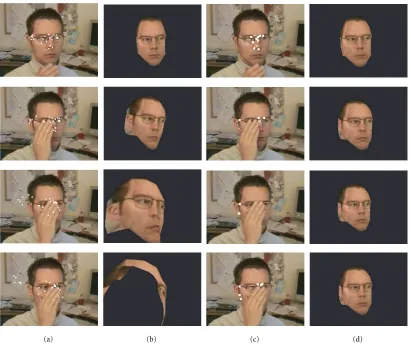
(a) (b) (c) (d)
Figure18: Occlusion robustness due to estimation of the measurement noise covariance matrix. Left: fixed covariance, resulting in mis-matched points (a) and lost track (b). Right: covariance estimated with the proposed method. Only points that are estimated to be small error cases are shown in (c). The tracking is almost unaffected (d).
Crowley and Berard [27] and by Olivier et al. [29]. By gath-ering statistics from the original texture (Figure 14a) in the areas likely to contain skin color (Figure 14b), the probability p(skin|x) that a pixel with colorxdepicts skin can be mod-eled as a Gaussian inYCrCbspace. The skin color probabil-ity can then be calculated and thresholded for every pixel in a subsampled version of the image (Figure 14c). A connected components processing step is performed on the binary im-age, and the biggest connected skin color blob is assumed to be the face (Figure 14d).
The skin color blob provides a very robust but not en-tirely accurate position of the head. To refine this posi-tion, a 13 × 13 template (Figure 15a) from the area be-tween the eyes is cropped out from a subsampled version of the original texture. The bounding box of the color blob is used as a search window for the template. Exhaustive search using normalized correlation is used in the search window, and the location of the maximum of the correla-tion (shown in Figure 15b) is used. Figure 15c shows a re-sult of the template matching. Since the texture between the eyes is situated in the middle of the face, it is visible even for relatively large out-of-plane rotations. Empirically,
it also works for comparatively large changes in scale. The model is then placed in the estimated position, facing the camera head-on and at the samezdistance as in the origi-nal initialization (Figure 15d). The tracker is then restarted and the Kalman filter will resolve the rotation and scale of the head for a rather large set of head poses. This is shown in Figure 16. The left-most image shows the video input at the time of reinitialization. The tracker is restarted in the position shown in the second image. After five iterations (about 0.2 second) the tracker has converged to the correct pose.
5. SYSTEM EVALUATION
000 060 120 180 240 300
Figure19: Example of tracking of a synthesized sequence where the motion is known. In each graph, the dashed curve represents the ground truth motion, and the solid curve represents the motion estimated from the tracker.
5.1. Robustness to occlusion
Due to the estimation of the measurement noise covariance matrix, the system is robust to occlusion of a large number of the feature points by, for example, a hand, as shown in the se-quence (Figure 18). Figures 18a and 18b show what happens when the covariance matrix is fixed; the estimated pose jerks severely and the track is often lost. With the proposed esti-mation of the covariance matrix, the tracking is almost com-pletely unaffected by the occlusion (Figures 18c and 18d). The sequence shown in Figure 18 is one of many such ex-amples.
5.2. Evaluation on synthetic data
To get an idea of the accuracy of the tracking, the follow-ing experiment has been conducted: first the tracker is run on a live image sequence to provide ground truth motion
ground truth is marked with a dashed curve and the tracked data is marked with a solid curve. The most striking system-atic error is that there is a delay between the ground truth and the estimates from zero to about ten frames (0.4 second). Also, at around frame 150, the error between the estimated parameters and the ground truth widens temporarily, as best seen in the Y translation and in quaternion 1, 2, and 4. Around frame 160, however, the estimates have recovered.
6. CONCLUSIONS
The SfM algorithm by Azarbayejani and Pentland has been analyzed for planar surfaces. Although the performance of the algorithm decreases for such surfaces, the behavior is not catastrophic and can be compared with measurement noise, poor depth priors, or low motion excitation. The algorithm is extended to handle new points, and it is then used in a head tracking system. Due to estimation of the covariance of the measurement noise, the system is robust to simultaneous oc-clusion of a large number of feature points. Furthermore, the system automatically detects tracking failure and performs a reinitialization using a color model and a template learned from the model. An experiment on synthetic data has also been conducted, showing a good following of the estimated parameters.
REFERENCES
[1] A. Azarbayejani and A. Pentland, “Recursive estimation of motion, structure, and focal length,” IEEE Trans. on Pattern Analysis and Machine Intelligence, vol. 17, no. 6, pp. 562–575, 1995.
[2] T. Jebara and A. Pentland, “Parametrized structure from mo-tion for 3D adaptive feedback tracking of faces,” inProc. IEEE Conference on Computer Vision and Pattern Recognition, pp. 144–150, San Juan, Puerto Rico, June 1997.
[3] M. J. Black and Y. Yacoob, “Recognizing facial expressions in image sequences using local parameterized models of image motion,” International Journal of Computer Vision, vol. 25, no. 1, pp. 23–48, 1997.
[4] S. Basu, Essa I., and A. Pentland, “Motion regularization for model-based head tracking,” inProc. 13th Int’l. Conf. on Pat-tern Recognition, vol. C, pp. 611–616, Vienna, Austria, August 1996.
[5] Y. Zhang and C. Kambhamettu, “Robust 3D head tracking under partial occlusion,” in4th International Conference on Face and Gesture Recognition, pp. 176–182, Grenoble, France, March 2000.
[6] P. Roivainen, Motion estimation in model-based coding of hu-man faces, Licentiate thesis, Link¨oping University, Sweden, 1990.
[7] M. Rydfalk, “CANDIDE, a parameterized face,” Tech. Rep. LiTH-ISY-I-0866, Link¨oping University, Sweden, Octo-ber 1987.
[8] H. Li, P. Roivainen, and R. Forchheimer, “3-D motion esti-mation in model-based facial image coding,” IEEE Trans. on Pattern Analysis and Machine Intelligence, vol. 15, no. 6, pp. 545–555, 1993.
[9] H. Li and R. Forchheimer, “Two-view facial movement esti-mation,” IEEE Trans. Circuits and Systems for Video Technol-ogy, vol. 4, no. 3, pp. 276–287, 1994.
[10] D. DeCarlo and D. Metaxas, “The integration of optical flow and deformable models with applications to human face
shape and motion estimation,” inProc. IEEE Conference on Computer Vision and Pattern Recognition, pp. 231–238, San Francisco, Calif, USA, June 1996.
[11] T. F. Cootes, G. J. Edwards, and C. J. Taylor, “Active appear-ance models,” inProc. European Conference on Computer Vi-sion 1998, H. Burkhardt and B. Neumann, Eds., vol. 2, pp. 484–498, Springer-Verlag, 1998.
[12] M. L. Cascia, S. Sclaroff, and V. Athitsos, “Fast, reliable head tracking under varying illumination: an approach based on registration of texture-mapped 3D models,” IEEE Trans. on Pattern Analysis and Machine Intelligence, vol. 22, no. 4, pp. 322–336, 2000.
[13] J. Ahlberg, “Facial feature tracking using an active appearance-driven model,” inProc. the EuroImage ICAV3D 2001 Conference, pp. 116–199, Mykonos, Greece, May 2001. [14] J. Str¨om, T. Jebara, S. Basu, and A. Pentland, “Real time
track-ing and modeltrack-ing of faces: an EKF-based analysis by synthesis approach,” inProc. the Modelling People Workshop at ICCV ’99, Corfu, Greece, August 1999.
[15] R. I. Hartley, “Ambiguous configurations for 3-view pro-jective reconstruction,” in Proc. 6th European Conference on Computer Vision, pp. 922–935, Dublin, Ireland, June–July 2000.
[16] G. P. Stein and A. Shashua, “On degeneracy of linear recon-struction from three views: linear line complex and applica-tions,” IEEE Trans. on Pattern Analysis and Machine Intelli-gence, vol. 21, no. 3, pp. 244–251, 1999.
[17] P. Torr, W. Fitzgibbon, and A. Zisserman, “Maintaining mul-tiple motion model hypotheses over many views to recover matching and structure,” inProc. 6th International Conf. on Computer Vision, pp. 485–491, Bombay, India, January 1998. [18] B. Triggs, “Autocalibration from planar scenes,” in Proc.
the 5th European Conference on Computer Vision, pp. 89–105, Freiburg, Germany, June 1998.
[19] J. Str¨om, “Structure from motion of planar surfaces, (analysis of an EKF based approach),” inProc. Symposium on Image analysis, Swedish Society for Automated Image Analysis, pp. 13– 16, Norrk¨oping, Sweden, March 2001.
[20] J. Str¨om, “Reinitialization of a model-based face tracker,” inProc. the EuroImage ICAV3D 2001 Conference, Mykonos, Greece, May 2001.
[21] J. Str¨om, T. Jebara, and A. Pentland, “Model-based real-time face tracking with adaptive texture update,” Tech. Rep. LiTH-ISY-R-2342, Link¨oping University, Sweden, March 2001. [22] A. Dell’Acqua, A. Sarti, and S. Tubaro, “Effective analysis
of image sequences for 3D camera motion estimation,” in Proc. the EuroImage ICAV3D 2001 Conference, pp. 307–310, Mykonos, Greece, May 2001.
[23] T. Jebara, A. Azarbayejani, and A. Pentland, “3D structure from 2D motion,” IEEE Signal Processing Magazine, vol. 16, no. 3, pp. 66–84, 1999.
[24] A. Gelb,Applied Optimal Estimation, MIT Press, Cambridge, 1996.
[25] S. Spanne,Lectures in Matrix Theory, Department of Mathe-matics, Lund Institute of Technology, Lund, Sweden, 1993. [26] C. E. Shannon, “A mathematical theory of communication,”
The Bell System Technical Journal, vol. 27, pp. 379–423, July, October 1948.
[27] J. L. Crowley and F. Berard, “Multi-modal tracking of faces for video communications,” inProc. IEEE Conference on Com-puter Vision and Pattern Recognition, pp. 640–645, San Juan, Puerto Rico, June 1997.
[29] N. Oliver, S. Pentland, and F. Berard, “LAFTER: a real-time lips and face tracker with facial expression recognition,” in Proc. IEEE Conference on Computer Vision and Pattern Recog-nition, pp. 123–129, San Juan, Puerto Rico, June 1997.
Jacob Str¨om received his M.S. degree in computer science and engineering at Lund Institute of Technology, Sweden, in 1995. He was a visiting Ph.D. student at Univer-sity of California, San Diego in 1995–1996, working for Prof. Pamela Cosman. In 1998, Str¨om received a Fulbright grant and spent one year as a visiting Ph.D. student at Prof. Alex Pentland’s Vision and Modeling group at the MIT Media Lab. In February 2002, he