FULL PAPER
On the modelling of M
2
tidal magnetic
signatures: effects of physical approximations
and numerical resolution
Jakub Velímský
1*, Alexander Grayver
2, Alexey Kuvshinov
2and Libor Šachl
1Abstract
The magnetic signatures of ocean M2 tides have been successfully detected by the low-orbit satellite missions CHAMP and Swarm. They have been also used to constrain the electrical conductivity in the uppermost regions of the Earth’s mantle. Here, we concentrate on the problem of accurate numerical modelling of tidally induced magnetic field, using two different three-dimensional approaches: the contraction integral equation method and the spherical har-monic-finite element method. In particular, we discuss the effects of numerical resolution, self-induction, the galvanic and inductive coupling between the oceans and the underlying mantle. We also study the applicability of a simplified two-dimensional approximation, where the ocean is approximated by a single layer with vertically averaged conduc-tivity and tidal forcing. We demonstrate that the two-dimensional approach is sufficient to predict the large-scale tidal signals observable on the satellite altitude. However, for accurate predictions of M2 tidal signals in the areas with significant variations of bathymetry, and close to the coastlines, full three-dimensional calculations are required. The ocean–mantle electromagnetic coupling has to be treated in the full complexity, including the toroidal magnetic field generated by the vertical currents flowing from and into the mantle.
Keywords: Electromagnetic induction, Ocean tides, Ocean-mantle electromagnetic coupling
© The Author(s) 2018. This article is distributed under the terms of the Creative Commons Attribution 4.0 International License (http://creat iveco mmons .org/licen ses/by/4.0/), which permits unrestricted use, distribution, and reproduction in any medium, provided you give appropriate credit to the original author(s) and the source, provide a link to the Creative Commons license, and indicate if changes were made.
Introduction
The phenomenon of electromagnetic fields induced in the Earth’s oceans by the motion of the conductive seawater in the presence of the main magnetic field has been known for decades (Sanford 1971). In particu-lar, the electromagnetic signatures of the ocean flows driven by the gravitational forcing of the Sun and the Moon have recently attracted an increased interest in the geomagnetic field community. Although the exist-ence of compound tides generated by nonlinear ocean dynamics is also well established (Einšpigel and Mar-tinec 2017), the fundamental part of tidal flows con-sists of the constituents present at discrete frequencies related to the movements of the celestial bodies. This attribute allows us to distinguish the tidally induced
magnetic field from the magnetic field originated in the Earth’s liquid core, in the lithosphere, or the external contributions from the magnetosphere and ionosphere, and their induced counterparts. Indeed, the magnetic signatures of the principal lunar semi-diurnal constitu-ent M2 , the larger lunar elliptic semi-diurnal
constitu-ent N2 , and partially also the lunar diurnal constituent O1 have been detected in ground geomagnetic obser-vatory data (Maus and Kuvshinov 2004) and seafloor measurements in the Northwestern Pacific (Schnepf et al. 2014). Similarly, the low-orbit satellite missions, such as CHAMP (Sabaka et al. 2015; Tyler et al. 2003) and Swarm (Sabaka et al. 2016), have successfully recovered the M2 and partially also the N2 tidally
induced magnetic signals. Other tidal signal, such as S2 ,
K1 , and P1 can be obscured by external fields (Guzavina
et al. 2018; Maus and Kuvshinov 2004). Consequently, the tidal signals extracted from satellite data were used to constrain the electrical conductivity across the litho-sphere–asthenosphere boundary (Grayver et al. 2016,
Open Access
*Correspondence: [email protected]
1 Department of Geophysics, Faculty of Mathematics and Physics, Charles University, V Holešovičkách 2, 180 00 Prague, Czech Republic
2017). Recently, Schnepf et al. (2018) have compared the numerical predictions of magnetic fields generated by oceanic and ionospheric tides. The idea to assimi-late the magnetic field measurements directly into the global ocean flow modelling has been implemented by Irrgang et al. (2017); however, tides were not consid-ered there. Another application of the forward model-ling of tidal signals is the construction of base functions optimized for tidal signal recovery from satellite and observatory data (Telschow et al. 2018).
The question of accurate calculation of the tidal mag-netic signatures embraces several problems. The choice of the tidal flow model from a plethora of purely hydro-dynamical or assimilative approaches definitely plays a role (Saynisch et al. 2018). The effect of the seawater conductivity and its seasonal variations has been dis-cussed by Saynisch et al. (2016). This paper returns back to the basic physical formulation of the problem of tid-ally induced magnetic fields. The two-dimensional (2-D) horizontal characteristics of the tidal flows were tradi-tionally exploited in the solution of the electromagnetic induction equation by assuming a 2-D conductive sheet of infinitesimal or finite thickness with a prescribed dis-tribution of 2-D imposed surface electric currents. Here, we refer to a recent detailed derivation by Tyler (2017) and references therein. Another level of simplification is related to the treatment of the underlying solid mantle.
In the simplest case, it is assumed to be a perfect insula-tor; more advanced methods allow for purely inductive, or inductive and galvanic coupling between the mantle and the ocean. Our paper aims to study the applicabil-ity of such simplifications using two state-of-the-art, fully three-dimensional (3-D) global modelling methods. Although the 3-D codes have been around for some time, only recently it has become computationally feasible to carry out such an analysis at sufficient resolutions. We do not attempt to play down the computational effec-tiveness of the approximate solutions. As discussed later in this manuscript, the computational costs of the fully 3-D solutions at high resolution are still prohibitive for inverse studies. Here, we merely test the validity of vari-ous physical approximations for modelling the magnetic field at the Earth’s surface and low-orbit satellite altitude induced by the principal lunar semi-diurnal constituent
M2.
The paper is organized as follows. We begin by recall-ing the 3-D formulation of the problem stemmrecall-ing from the quasi-stationary Maxwell equations and proceed to a 2-D approximation. We then look at the effects of elec-tromagnetic interaction of the ocean and mantle, treating separately the galvanic and inductive coupling. Using two independent solutions ensures that the observed effects correspond to real physical phenomena and issues of
−100 −50 0 50 100
Re U (m2/s)
−100 −50 0 50 100
Im U (m2/s)
−100 −50 0 50 100
Re V (m2/s)
−100 −50 0 50 100
Im V (m2/s)
implementation, resolution, and numerical accuracy are clearly separated.
Tidally induced magnetic field in the Earth’s oceans
The three‑dimensional electromagnetic induction equation
The magnetic field B(r;t) and the electric field E(r;t) induced in the Earth’s oceans by the motion of the salt-water in the presence of the Earth’s main magnetic field BM(r;t) are governed by the quasi-static Maxwell equations,
Here, µ0 is the magnetic permeability of vacuum. The
electric current density j(r;t) is related to the electric field through the Ohm’s law,
(1)
with σ (r) representing the electrical conductivity, in
gen-eral both latgen-erally and radially varying. The imposed elec-tric current density jimp(r;t) and the imposed electric field Eimp(r;t) are defined as
Here, u(r;t) is the spatially and temporally dependent velocity of the ocean flow. In general, it is fully three-dimensional (3-D), containing all three vector compo-nents varying along all three dimensions in the oceans. The same equations with zero imposed electric field or current also hold in the conductive Earth’s mantle. We have implicitly assumed that BM is a potential field, its amplitude is much larger than that of the induced field, and its time variations are too slow to be considered in the diffusion process. At the Earth surface, r=a , the
induced magnetic field is coupled to a scalar magnetic potential U(r;t),
log10(Conductivity in S/m) 0
log10(Surface conductance in S)
r=6369.9250 km
that satisfies the Laplace equation in the insulating atmosphere, and assuming the absence of external sources, it disappears as r→ ∞.
Since the tidal flows are dominated by signals at discrete frequencies, it is common to reformulate the problem in the frequency domain. Assuming the exp(−iωt)
depend-ence of the velocities and induced fields, and ignoring the notation distinction between time-domain and frequency-domain variables, we write
In this paper, we consider only the principal lunar semi-diurnal constituent M2 with a period of 12.42 h, and thus
angular frequency ω=1.4×10⁻⁴rad/s . This component has by far the largest magnetic signatures, which have been reliably detected by satellite observations (Sabaka et al. 2016).
The Ampère and the Faraday laws (7–8) can be com-bined with Eqs. (4) and (5) into a single second-order electromagnetic induction (EMI) equation for the mag-netic field vector B,
Because of linearity, the induction caused by external sources in the ionosphere and magnetosphere represents an independent solution, which is not considered here, and we refer to a comprehensive benchmark of externally induced magnetic fields by Kelbert et al. (2014).
The solution of Eqs. (7–8) or (10) in the computational domain comprising the oceans and the solid Earth below is a challenging task, in particular in the presence of large lateral variations of conductivity, which coincide with the spatial distribution of the source term on the right-hand side. Here, we employ two numerical methods.
The elmgFD code uses the spherical harmonic-finite element approach, introduced by Martinec (1999), to solve the EMI Eq. (10). It has been recently rewritten using modern parallelized FFT and LAPACK librar-ies, the BiCGStab(2) iterative solver (Sleijpen and Fok-kema 1993), applying an effective pre-conditioner based on the spherical harmonic solution of the 1-D problem (Martinec 1999), and incorporating the zero external field boundary condition (6) at the Earth–atmosphere interface (Velímský and Martinec 2005), and the inter-nal forcing (5). The lateral resolution is controlled by the maximum spherical harmonic degree jmax . The code is very effective in terms of memory usage, avoiding the
(7)
storage of the full problem matrix. At the highest reso-lution employed here, jmax=480 with 102 3-D layers in
the oceans, and additional 100 1-D layers in the mantle, the calculation of one forward run required 30 GiB of memory and took about 2 days on a 12-core modern PC. Note that the memory requirements scale linearly with the total number of layers and quadratically with jmax . The duration of a single iteration scales with the third power of jmax and linearly with the number of 3-D lay-ers. Obviously, the total number of iterations depends on the requested accuracy, and convergence rate can be influenced also by the range of lateral conductivity vari-ations. In general, the presented results are at the edge of practicality for single-frequency forward calculations. When employed in the inverse modelling, significant reduction of lateral and radial resolution is needed. For accurate transformations between the spatial and spheri-cal harmonic domains by means of the Gauss–Legendre quadrature, the electrical conductivity, the tidal flows, and the solution itself are distributed on an irregular grid
elmgFD jmax=120
Fig. 3 Geomagnetic power spectra. Geomagnetic power spectra at the Earth surface (solid lines and symbols) and at the satellite altitude of 400 km (dashed lines). Results of the 2-D approaches elmgFD and
in colatitude, and bilinear interpolation is used for con-versions to and from a regular grid.
The x3dg (Kuvshinov 2008) code is based on the con-tracting integral equation (CIE) approach (Pankratov et al. 1995; Singer 1995). Within the approach, the Max-well Eqs. (7, 8) are transformed to CIE which is solved using Krylov subspace iterations with pre-calculated Green tensors for a 1-D medium. The approach allows for computing the EM fields in the Earth’s models with fully 3-D conductivity distributions. One of the advantages of the x3dg method lies in the fast iterative process with guaranteed convergence, as the condition number of the
system matrix depends only on the square root of maxi-mum lateral conductivity contrast. On the other hand, it is partially offset by the large memory requirements of the Green tensors in the current implementation and lack of parallelization for single-frequency calculations. For example, using a single ocean layer at 0.25◦ lateral resolution requires over 100 GiB of memory or swap disc space with corresponding speed penalty. The memory requirements scale quadratically with the number of 3-D layers and latitudinal resolution, quickly saturating even the most advanced shared-memory architecture available today.
−2 0 2
Re X (nT)
−2 0 2
Im X (nT)
−2 0 2
Re Y (nT)
−2 0 2
Im Y (nT)
−4 −2 0 2 4
Re Z (nT)
elmgFD jmax=480
−4 −2 0 2 4
Im Z (nT)
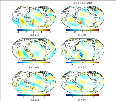
Fig. 4 Magnetic signatures of M2 tides. The real (left column) and the imaginary (right column) parts of the three magnetic field components at the Earth’s surface calculated using the elmgFD code with 2-D surface conductance and forcing at the highest lateral resolution, jmax=480 . Note the
The three‑dimensional and the two‑dimensional approaches
The gravitational forcing that drives the tidal flows is almost independent of the vertical coordinate in the ocean, and therefore, the ocean tides are usually mod-elled in the two-dimensional (2-D) barotropic approxi-mation (Hendershott 1973). The full velocity field u(r) for a given tidal constituent is not calculated, and only the horizontal transport is available. It is defined as a vertical integral of the horizontal velocity uH,
(11) U(ϑ,ϕ)=
a
a−b(ϑ,ϕ)
uH(r,ϑ,ϕ)dr,
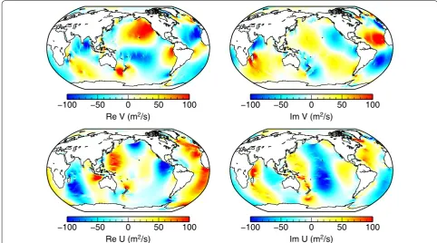
where b(ϑ,ϕ) represents the local bathymetry at colati-tude and longicolati-tude (ϑ,ϕ) . The small contribution associ-ated with laterally varying surface elevation is neglected in Eq. (11). Figure 1 shows the M2 transport from an
assimilative barotropic model TPXO8-atlas (Egbert and Erofeeva 2002) that has been used in this study.
The vertical velocity component stemming from the baroclinic internal tides (Kantha and Tierney 1997) is not considered here. A reliable baroclinic tidal model with assimilated altimetry data has not been pub-lished yet. Besides, the frequency shift and spread of baroclinic tides would require a multi-frequency or time-domain approach to the solution of the induction Eq. (10), a task out of the scope of the present paper.
−0.5 0.0 0.5
Re ∆X (nT)
−0.5 0.0 0.5
Im ∆X (nT)
−0.5 0.0 0.5
Re ∆Y (nT)
−0.5 0.0 0.5
Im ∆Y (nT)
−0.5 0.0 0.5
Re ∆Z (nT)
elmgFD 2D−x3dg 2D
−0.5 0.0 0.5
Im ∆Z (nT)
In order to calculate the tidally induced magnetic fields in the 3-D settings, we need to specify the dis-tribution of electrical conductivity in the uppermost layers, comprising the oceans, the continents, and the underlying crust, σ3D(r,ϑ,ϕ) . In the present paper, we
start with a simplified approach, based on only two val-ues of electrical conductivity: one for the seawater and one for the solid crust,
with b(ϑ,ϕ)=0 at the continents. Here, h=8000 km is the ocean layer thickness, which should be larger than
(12) σ3D(r,ϑ,ϕ)=
σocean=3.2S/m for r≥a−b(ϑ,ϕ),
σcrust=0.001S/m for a−h≤r<a−b(ϑ,ϕ),
the maximum bathymetry. The actual value of σcrust has only small influence on the tidally induced magnetic fields, spatially limited to coastal areas.
An alternative approach introduces a 3-D electri-cal conductivity distribution σ3D(T,s) which is based on
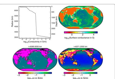
the collocated seawater temperature and salinity (T, s) measurements (Tyler et al. 2017). Variable thickness of ocean, continental, and shelf sediments is also incorpo-rated along the lines presented by Everett et al. (2003). Two cross sections of σ3D(T,s) are shown in the bottom
panels of Fig. 2. Near the surface, the seawater conduc-tivity shows significant variations with colatitude. In the deep oceans, the lateral variations are suppressed.
−0.5 0.0 0.5
Re ∆X (nT)
−0.5 0.0 0.5
Im ∆X (nT)
−0.5 0.0 0.5
Re ∆Y (nT)
−0.5 0.0 0.5
Im ∆Y (nT)
−0.5 0.0 0.5
Re ∆Z (nT)
elmgFD 3D−elmgFD 2D
−0.5 0.0 0.5
Im ∆Z (nT)
Fig. 6 Effect of dimensionality. Differences between the 3-D and 2-D solutions calculated at the Earth’s surface with the elmgFD code at
In order to construct the 3-D structure of the imposed electric currents or electric fields, we assume that the horizontal ocean velocity is constant within the entire ocean column. Then, we obtain from (11),
for a−b(ϑ,ϕ)≤r≤a , and zero elsewhere. The hori-zontal transport (11) is conserved, and Eq. (5) can be used to calculate the 3-D imposed electric field or electric current. While the velocity field calculated by Eq. (13)
(13) u3D(r,ϑ,ϕ)= U(ϑ,ϕ)
b(ϑ,ϕ),
has only the horizontal components, its spatial distribu-tion follows the bathymetry profile.
In the two-dimensional approach, the radial conduc-tivity profile is averaged and replaced with a scaled, two-dimensional conductivity map
Similarly, the imposed currents are also vertically integrated,
(14)
σ2D(ϑ,ϕ)= 1
h a
a−h
σ3D(r,ϑ,ϕ)dr.
−0.5 0.0 0.5
Re ∆X (nT)
−0.5 0.0 0.5
Im ∆X (nT)
−0.5 0.0 0.5
Re ∆Y (nT)
−0.5 0.0 0.5
Im ∆Y (nT)
−0.5 0.0 0.5
Re ∆Z (nT)
elmgFD 3D (temp+sal+sed)−elmgFD 2D
−0.5 0.0 0.5
Im ∆Z (nT)
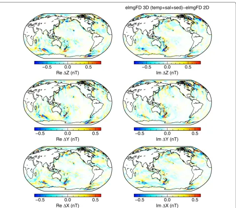
Fig. 7 Effect of variable seawater conductivity and sediments. Differences between the 3-D and 2-D solutions calculated at the Earth’s surface with the elmgFD code at jmax=480 . The 3-D solution includes temperature and salinity-dependent seawater conductivity and variable sediment
under the assumption that the radial variabil-ity of the main field across the ocean is negligible,
BM(r,ϑ,ϕ)≈BM(a,ϑ,ϕ) . The imposed electric fields are then expressed as
Note that the calculation of Eimp2D via Eq. (16) assures consistency between the Maxwell Eqs. (7–8) and the EMI Eq. (10). On the other hand, setting simply Eimp2D =U×BM/h does not.
The 2-D approach presented here only suppresses the radial variations of conductivity and imposed currents in the oceans. The formulation still includes both the gal-vanic and inductive coupling with the underlying mantle. This is in contrast with the 2-D approach by Tyler (2017), where the galvanic coupling is omitted.
Inductive and galvanic interaction with the underlying mantle
One of the goals of this study is to assess the importance of both inductive and galvanic coupling of the ocean magnetic field with the underlying conductive man-tle. We use a recent global 1-D electrical conductivity model by Grayver et al. (2017), derived from Swarm and CHAMP satellite data using a combination of magne-tospheric and tidal forcing. The profile, as shown in the upper left panel of Fig. 2, features an abrupt increase in electrical conductivity across the lithosphere–asteno-sphere boundary. The conductivity further increases in the transition zone in the upper mantle. A highly conduc-tive core is also included in the model.
Two models with limited physics are calculated by both numerical methods to study the ocean–mantle interac-tions. In the so-called decoupled model, the galvanic cou-pling is removed. In x3dg, it is achieved by inserting a 100-m thin layer with electrical conductivity of 10−12S/m between the ocean and the mantle. The spherical har-monic approach elmgFD allows us to directly disable the toroidal magnetic field and hence any radial electric cur-rents. Only the inductive interaction between the oceans and the mantle is preserved.
The second model, marked as insulated in the follow-ing figures and discussion, assumes an insulatfollow-ing man-tle below the ocean. In elmgFD, a perfectly insulating
(15)
x3dg both for the mantle and the core. Hence, the effect of mantle conductivity is completely suppressed.
Results
Effect of lateral resolution and dimensionality
In the first series of runs, we have calculated the mag-netic signatures of the TPXO8-atlas M2 tides using the elmgFD and x3dg codes with the 2-D settings and full physics. The electrical conductivity was assembled according to Eq. (14), and the elmgFD and x3dg solu-tions were, respectively, forced by the imposed electric field (16) or electric current (15). The spherical harmonic truncation degree of elmgFD was set in turn to 120, 240, and 480. Similarly, the lateral resolution of x3dg was increased from 1◦×1◦ to 0.5◦×0.5◦ and finally
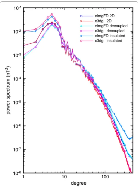
Fig. 8 Effect of physical approximations on the geomagnetic power spectra. Geomagnetic power spectra calculated at the Earth surface by the 2-D approaches elmgFD and x3dg, and the respective effects of galvanically decoupled and insulated mantle. The lateral resolution was kept at jmax=480 and 0.25◦
calculated by elmgFD at the highest lateral resolution and discretizing the ocean radially into 40 and 102 lay-ers, respectively, for the conductivity models σ3D and
σ3D(T,s) . The imposed electric field was calculated using Eq. (5) with quasi-3-D flows assembled according to Eq. (13). The large memory demands of x3dg have so far prevented us from calculating such high-resolution 3-D solutions with this code.
Figure 3 shows the power spectra of the tidally induced field at the Earth’s surface, and at the altitude of 400 km, typical for low-orbit satellite missions such as Swarm. The spectra were calculated using the formula by Maus (2008,
eq. 21), taking into account the increasing number of coefficients with the spherical harmonic degree. The maximum average power is present at degree five. The spectra follow the power law for degrees above 10 with-out reaching a plateau. That suggests that the induced field remains correlated across different spatial scales. At the lowest resolution, we can observe significant differ-ences between the 2-D and 3-D methods, diverging for higher spherical harmonic degrees. An interesting obser-vation is that the elmgFD method predicts systematically larger spectra than the x3dg method. As the lateral reso-lution increases, the differences between both methods
−1 0 1
Re ∆X (nT)
−1 0 1
Im ∆X (nT)
−1 0 1
Re ∆Y (nT)
−1 0 1
Im ∆Y (nT)
−2 −1 0 1 2
Re ∆Z (nT)
elmgFD 2D−elmgFD decoupled
−2 −1 0 1 2
Im ∆Z (nT)
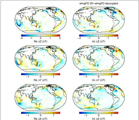
Fig. 9 Effect of galvanically decoupled mantle. Differences between the 2-D solution and a unimodal solution without toroidal magnetic field, i.e. galvanically decoupled from the underlying conductive mantle. Both solutions were calculated at the Earth’s surface with the elmgFD code at
are reduced. A possible explanation lies in the use of global base functions in elmgFD, compared to a local discretization applied in x3dg. Truncating the elmgFD solution at a lower degree prevents additional diffusion of magnetic field energy into higher degrees and hence increases the spectrum.
Figure 4 shows the M2 signatures predicted by the elmgFD code at the highest resolution of spherical har-monic degree 480. The magnetic field components are in general agreement with previous studies. We will use this
figure as a reference to demonstrate the various effects with difference plots.
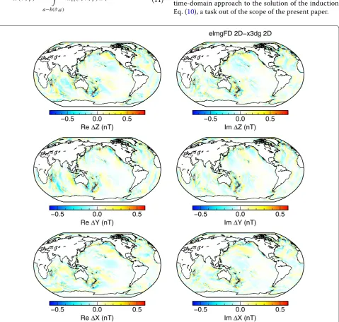
First such difference is plotted in Fig. 5 where the 2-D solutions of elmgFD and x3dg at their respective high-est resolutions are compared. As can be expected, the largest differences in all three components are concen-trated in the areas where spatially complex tidal flows interact with strong vertical main magnetic field, such as in the Tasman sea and further south and east of New
−1 0 1
Re ∆X (nT)
−1 0 1
Im ∆X (nT)
−1 0 1
Re ∆Y (nT)
−1 0 1
Im ∆Y (nT)
−2 −1 0 1 2
Re ∆Z (nT)
elmgFD 2D−elmgFD insulator
−2 −1 0 1 2
Im ∆Z (nT)
Zealand. Even there, the differences stay below 10% of the total predicted signal.
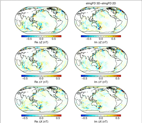
The effect of dimensionality is shown in the differ-ence plots in Figs. 6 and 7. The 3-D elmgFD solutions differ from the 2-D solution obtained by the same code mostly in the shallow areas, such as the Kerguelen pla-teau in the southern Indian ocean, the Bering sea, or the Rockall plateau in the northern Atlantic. In the more complicated σ3D(T,s) model, the differences are
slightly amplified, and detailed patterns of magnetic fields are modified, e.g. in the Weddell Sea, the Tas-man Sea, and in the northern Atlantic. In these areas, the prediction of the 2-D model can be of even by 50%
of the signal amplitudes. In view of these results, the 2-D approximation seems to be acceptable over deep oceans, where the differences are only slightly larger than those related to the choice of the modelling code.
Effect of conductive mantle on the tidal signatures
The effects of galvanic decoupling of the mantle and the insulating mantle are shown in Fig. 8 by means of power spectra at the Earth’s surface. In spite of imple-mentation differences in both methods, the behaviour is consistent. For the decoupled model, the power spec-tra are reduced for degrees one to six and increased from degree seven onwards. This is in agreement with
−0.005 0.000 0.005
Re jr (µA/m2)
−0.005 0.000 0.005
Im jr (µA/m2)
−2 −1 0 1 2
Re jϑ (µA/m2)
−2 −1 0 1 2
Im jϑ (µA/m2)
−2 −1 0 1 2
Re jϕ (µA/m2)
elmgFD 2D
−2 −1 0 1 2
Im jϕ (µA/m2)
Fig. 11 Electric current density at the seafloor. The eastward, southward, and radial components of the 2-D elmgFD solution at jmax=480 are
the theoretical arguments in Tyler (2017, Section 5.5). The spatial structure of the differences between the full 2-D model and the decoupled model is shown in Fig. 9. It is concentrated into the coastal areas, with the larg-est differences pronounced around southern Africa, on the Australian eastern coast, in the Labrador Basin, and west of the British Isles.
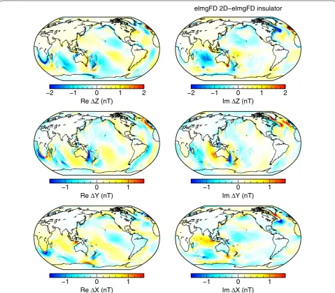
In the case of insulating mantle, the effects become even more interesting. Judging from the spectra in Fig. 8, the amplitude of the signal is increased, espe-cially at the lower degrees. The spatial pattern of dif-ferences, as displayed in Fig. 10, repeats most of the features from Fig. 9. However, the magnetic field is significantly strengthened over the deep oceans, miss-ing the counteractmiss-ing field generated by the large-scale induced currents in the mantle. This effect is evidently stronger than the galvanic coupling, shifting the entire spectrum upwards.
Another view on the full 2-D, the decoupled, and the insulated solutions is provided by means of electric current density at the seafloor, as plotted, respectively, in Figs. 11, 12 and 13. The vertical currents, which are
present only in the full solution, are concentrated in the coastal areas. The pattern of the horizontal electric cur-rents is changed and the amplitude mostly weakened in both the decoupled and insulated solutions.
Conclusions
The recent advances in 3-D EM modelling allow us to calculate the magnetic signatures of the ocean tides in high resolution and in the full complexity. However, vari-ous physical approximations still can provide significant reduction of computational time and/or memory require-ments, which can be exploited, especially in the inver-sion scenarios. We have evaluated the effect of various traditional approximations. The predictions of the 2-D approach match well with the 3-D approach locally above deep oceans, or in the interpretation of low-orbit satellite data dealing with spherical harmonic degrees below 20. However, for accurate prediction of signals at the coastal and island geomagnetic observatories, or more generally, in the areas with significant variations of bathymetry and coastlines, full 3-D calculations still may be required. This
−2 −1 0 1 2
Re jϑ (µA/m2)
−2 −1 0 1 2
Im jϑ (µA/m2)
−2 −1 0 1 2
Re jϕ (µA/m2)
elmgFD decoupled
−2 −1 0 1 2
Im jϕ (µA/m2)
conclusion does not confirm the argument presented by Tyler (2017, Section 5.2) that the Earth oceans behave as an electrically thin sheet for periods above 10 min. Note that Tyler’s criterion is based on the penetration depth of magnetic field from the boundary. However, the imposed electric currents are distributed everywhere in the ocean volume and for tidal movements do not decrease signifi-cantly with depth.
The 3-D approach presented here is still based on the 2-D barotropic tidal flows. The prediction of the mag-netic field induced by the 3-D tidal flows comprising the baroclinic component (Stammer et al. 2014) has not yet been performed. Although the comparison of Say-nisch et al. (2018) includes several baroclinic models, the induced magnetic field was still calculated from horizon-tal transports only.
The electromagnetic interactions of the oceans with the underlying conductive mantle are significant enough to be treated comprehensively in numerical model-ling, including the galvanic coupling and possibility of vertical electric currents flowing from or into the man-tle. The omission of the galvanic coupling leads to an underestimation of the tidal signals at degrees below six, in agreement with the analytical estimates by Tyler
(2017, Section 5.5). Using a completely insulating mantle has the opposite effect.
Authors’ contributions
JV carried out the calculations using his own elmgFD code and the x3dg code, with support from AG and AK (its original author). LŠ contributed to data preparation and testing of the elmgFD code. JV was responsible for produc-ing the figures and writproduc-ing the manuscript with discussions and contributions from all other authors. All authors read and approved the final manuscript.
Author details
1 Department of Geophysics, Faculty of Mathematics and Physics, Charles University, V Holešovičkách 2, 180 00 Prague, Czech Republic. 2 Institute of Geophysics, ETH Zurich, Sonneggstrasse 5, 8092 Zurich, Switzerland.
Acknowledgements
This research was supported by the Grant Agency of the Czech Republic, Project No. P210/17-03689S, the Charles University Grant SVV 115-09/260447, and the European Space Agency Contract No. 4000109562/14/NL/CBi ‘Swarm+Oceans’. The computational resources were provided by The Ministry of Education, Youth and Sports from the Large Infrastructures for Research, Experimental Development and Innovations Project “IT4Innovations National Supercomputing Center—LM2015070”, Project ID OPEN-13-21. We thank R. Tyler, L. Erofeeva, and G. Egbert for making the 3-D electrical conductivity and the TPXO8 datasets, respectively, freely available. We also thank R. Tyler and an anonymous reviewer for their helpful comments.
Competing interests
The authors declare that they have no competing interests.
−2 −1 0 1 2
Re jϑ (µA/m2)
−2 −1 0 1 2
Im jϑ (µA/m2)
−2 −1 0 1 2
Re jϕ (µA/m2)
elmgFD insulated
−2 −1 0 1 2
Im jϕ (µA/m2)
Publisher’s Note
Springer Nature remains neutral with regard to jurisdictional claims in pub-lished maps and institutional affiliations.
Received: 10 September 2018 Accepted: 3 December 2018
References
Egbert GD, Erofeeva SY (2002) Efficient inverse modeling of barotropic ocean tides. J Atmos Ocean Technol 19(2):183–204
Einšpigel D, Martinec Z (2017) Time-domain modelling of global ocean tides generated by the full lunisolar potential. Ocean Dyn 67:165–189. https :// doi.org/10.1007/s1023 6-016-1016-1
Everett ME, Constable S, Constable C (2003) Effects of near-surface conduct-ance on global satellite induction responses. Geophys J Int 153:277–286 Grayver AV, Schnepf NR, Kuvshinov AV, Sabaka TJ, Manoj C, Olsen N (2016)
Satellite tidal magnetic signals constrain oceanic lithosphere–astheno-sphere boundary. Sci Adv 2:1600798
Grayver AV, Munch FD, Kuvshinov AV, Khan A, Sabaka TJ, Tøffner-Clausen L (2017) Joint inversion of satellite-detected tidal and magnetospheric signals constrains electrical conductivity and water content of the upper mantle and transition zone. Geophys Res Lett 44:6074–6081
Guzavina M, Grayver A, Kuvshinov A (2018) Do ocean tidal signals influence recovery of solar quiet variations? Earth Planets Space 70(1):5. https ://doi. org/10.1186/s4062 3-017-0769-1
Hendershott MC (1973) Ocean tides. Eos Trans Am Geophys Union 54(2):76–86 Irrgang C, Saynisch J, Thomas M (2017) Utilizing oceanic electromagnetic
induction to constrain an ocean general circulation model: a data assimi-lation twin experiment. J Adv Model Earth Syst 9(3):1703–1720. https :// doi.org/10.1002/2017M S0009 51
Kantha LH, Tierney CC (1997) Global baroclinic tides. Prog Oceanogr 40(1):163–178. https ://doi.org/10.1016/S0079 -6611(97)00028 -1 Tidal Sci-ence In Honour of David E. Cartwright
Kelbert A, Kuvshinov A, Velímský J, Koyama T, Ribaudo J, Sun J, Martinec Z, Weiss CJ (2014) Global 3-D electromagnetic forward modelling: a bench-mark study. Geophys J Int 197:785–814
Kuvshinov AV (2008) 3-D global induction in the oceans and solid earth: recent progress in modeling magnetic and electric fields from sources of magnetospheric, ionospheric and oceanic origin. Surv Geophys 29(2):139–186. https ://doi.org/10.1007/s1071 2-008-9045-z
Martinec Z (1999) Spectral-finite element approach to three-dimensional elec-tromagnetic induction in a spherical earth. Geophys J Int 136:229–250 Maus S, Kuvshinov A (2004) Ocean tidal signals in observatory and satellite
magnetic measurements. Geophys Res Lett 31:15313
Maus S (2008) The geomagnetic power spectrum. Geophys J Int 174(1):135– 142. https ://doi.org/10.1111/j.1365-246X.2008.03820 .x
Pankratov OV, Avdeev DB, Kuvshinov AV (1995) Scattering of electromagnetic field in inhomogeneous earth: forward problem solution. Izv Akad Nauk SSSR Fiz Zemli 3:17–25
Sabaka TJ, Tyler RH, Olsen N (2016) Extracting ocean-generated tidal magnetic signals from Swarm data through satellite gradiometry. Geophys Res Lett 43:3237–3245
Sabaka TJ, Olsen N, Tyler RH, Kuvshinov A (2015) CM5, a pre-Swarm compre-hensive geomagnetic field model derived from over 12 year of CHAMP, Ørsted, SAC-C and observatory data. Geophys J Int 200:1596–1626 Sanford TB (1971) Motionally induced electric and magnetic fields in the sea. J
Geophys Res 76:3476–3492
Saynisch J, Irrgang C, Thomas M (2018) Estimating ocean tide model uncer-tainties for electromagnetic inversion studies. Ann Geophys 36(4):1009– 1014. https ://doi.org/10.5194/angeo -36-1009-2018
Saynisch J, Petereit J, Irrgang C, Kuvshinov A, Thomas M (2016) Impact of climate variability on the tidal oceanic magnetic signal-a model-based sensitivity study. J Geophys Res Oceans 121(8):5931–5941. https ://doi. org/10.1002/2016J C0120 27
Schnepf NR, Manoj C, Kuvshinov A, Toh H, Maus S (2014) Tidal signals in ocean-bottom magnetic measurements of the northwestern pacific: observa-tion versus predicobserva-tion. Geophys J Int 198:1096–1110
Schnepf NR, Nair M, Maute A, Pedatella NM, Kuvshinov A, Richmond AD (2018) A comparison of model-based ionospheric and ocean tidal magnetic signals with observatory data. Geophys Res Lett 45(15):7257–7267. https ://doi.org/10.1029/2018G L0784 87
Singer B (1995) Method for solution of Maxwell’s equations in non-uniform media. Geophys J Int 120:590–598
Sleijpen GLG, Fokkema DR (1993) BiCGstab (l) for linear equations involving unsymmetric matrices with complex spectrum. Electron Trans Numer Anal 1:11–32
Stammer D, Ray R, Andersen OB, Arbic B, Bosch W, Carrère L, Cheng Y, Chinn D, Dushaw B, Egbert G et al (2014) Accuracy assessment of global baro-tropic ocean tide models. Rev Geophys 52(3):243–282
Telschow R, Gerhards C, Rother M (2018) On the approximation of spa-tial structures of global tidal magnetic field models. Ann Geophys 36(5):1393–1402. https ://doi.org/10.5194/angeo -36-1393-2018
Tyler RH, Maus S, Lühr H (2003) Satellite observations of magnetic fields due to ocean tidal flow. Science 299:239–241
Tyler RH (2017) Mathematical modeling of electrodynamics near the surface of earth and planetary water worlds. In: Technical report TM-2017-219022, NASA. https ://ntrs.nasa.gov/archi ve/nasa/casi.ntrs.nasa.gov/20170 01127 9.pdf. Accessed 8 Nov 2018
Tyler RH, Boyer TP, Minami T, Zweng MM, Reagan JR (2017) Electrical conduc-tivity of the global ocean. Earth Planets Space 69:156