Study on Mathematical Modeling of Power System Stability Analysis

(1)

ISSN (Print) : 2320 – 3765 ISSN (Online): 2278 – 8875

I

nternational

J

ournal of

A

dvanced

R

esearch in

E

lectrical,

E

lectronics and

I

nstrumentation

E

ngineering

(An ISO 3297: 2007 Certified Organization)

Vol. 5, Issue 6, June 2016

Study on Mathematical Modeling of Power

System Stability Analysis

Gulvender, Priyajit Dash

M.Tech. Student, Department of EEE, BRCM College of Engineering, Behal, Bhiwani Haryana, India Asst. Professor, Department of EEE, BRCM College of Engineering, Behal, Bhiwani Haryana, India

ABSTRACT: A power system is the breath of today infrastructure which is controlled by various methods and to handle a system smartly it is necessary to know about its various parameters and role played by them. It is the tendency of every system in whole universe to attain a state where system gets stable. In this paper we study various mathematical modeling of power system in aspect of analyzing the stability of the system. A brief classification of the system stability is described and mathematical equation for the stability analysis are presented which will be helpful in understanding the system behavior and fault analysis of multi machine power system.

I. INTRODUCTION

A power system consists of three stages known as generation, transmission, and distribution. In the first stage, generation, the electric power is generated mostly by using synchronous generators. Then the voltage level is raised by transformers before the power is transmitted in order to reduce the line currents which consequently reduce the power transmission losses. After the transmission, the voltage is stepped down using transformers in order to be distributed accordingly.

Power systems are designed to provide continuous power supply that maintains voltage stability. However, due to undesired events, such as lightning, accidents or any other unpredictable events, short circuits between the phase wires of the transmission lines or between a phase wire and the ground which may occur is called a fault. Due to occurring of a fault, one or more generators may be severely disturbed causing an imbalance between generation and demand. If the fault persists and is not cleared in a pre-specified time frame, it may cause severe damages to the equipments which in turn may lead to a power loss and power outage. Therefore, protective equipments are installed to detect faults and clear/isolate faulted parts of the power system as quickly as possible before the fault energy is propagated to the rest of the system.

Random changes in load are taking place at all times, with subsequent adjustments of generation. We may look at any of these as a change from one equilibrium state to another. Synchronism frequently may be lost in that transition period, or growing oscillations may occur over a transmission line, eventually leading to its tripping. These problems must be studied by the power system engineer and fall under the heading "power system stability".

1.1Power System Stability

The tendency of a power system to develop restoring forces equal to or greater than the disturbing forces to maintain the state of equilibrium is known as “STABILITY”. Stability phenomenon is a single problem associated with various forms of instabilities affected on power system due to the high dimensionality and complexity of power system constructions and behaviors.

(2)

I

nternational

J

ournal of

A

dvanced

R

esearch in

E

lectrical,

E

lectronics and

I

nstrumentation

E

ngineering

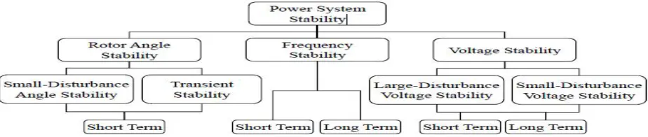
Figure 1.1 Classification of stability based on IEEE/CIGRE joint task force on stability

1.1 Rotor Angle Stability

Rotor angle stability is concerned with the ability of interconnected synchronous machines of a power system to remain in synchronism under normal operating conditions and after being subjected to a disturbance [9]. The stability of synchronous machines depends on the ability of restoring the equilibrium between their electromagnetic outputs torques and the mechanical input torques and keeping at synchronize with other machines following a major disturbance such as short circuit. Under steady state conditions, there is equilibrium between the input mechanical torque and the output electromagnetic torque of each generator, and the speed remains constant. If the system is perturbed, this equilibrium is upset and instability may occur in the form of increasing or decreasing angular swings of some generators leading to their loss of synchronism with other generators. The change in electrical torque ΔT of a

synchronous machine following a perturbation can be resolved into two components as follows [13]:

= ∆ + ∆ (1)

Where ∆ is the component of torque change in phase with the rotor angle perturbation ∆ and it is referred to as synchronizing torque component. is the synchronizing torque coefficient. ∆ is the component of torque change

in phase with the speed deviation Δω and it is referred to damping torque component. is the damping torque coefficient.

Stability of each machine in the system depends on the existence of both components. Lack of sufficient synchronizing torque produces instability through aperiodic or non-oscillatory drift in the rotor angle, whereas lack of damping torque results in oscillatory instability causes rotor oscillating with increasing amplitude. Rotor angle stability depends on the initial operating state and the severity of the disturbance on synchronous machines. Commonly, rotor angle stability are classified into small disturbance-rotor angle stability and large disturbance-rotor angle stability for gaining more understanding and insights into the nature and characteristics of stability problem.

1.2 Voltage Stability

Voltage stability refers to the ability of a power system to maintain steady voltages at all buses in the system after being subjected to a disturbance from a given initial operating condition [13]. The voltage deviations need to maintain within predetermined ranges. A voltage stability problem occurs in heavily stressed systems, which associated with long transmission lines. Voltage stability depends on the active and reactive power balance between load and generation in the entire power system and the ability to maintain/restore this balance during normal and abnormal operation. The main contributor in voltage instability is the increase of reactive power requirements beyond the sustainable capacity of the available reactive power resources when some of the generators hit their field or armature current time-overload capability limits. The other contributor is the extreme voltage drop that occurs when active and reactive power flow through inductive reactance of the transmission network; this limits the capability of the transmission network for power transfer and voltage support.

(3)

I

nternational

J

ournal of

A

dvanced

R

esearch in

E

lectrical,

E

lectronics and

I

nstrumentation

E

ngineering

over-voltage instability problem at some buses due to the capacitive behavior of the network and under excitation limiters that preventing generators and synchronous compensators from absorbing excess reactive power in the system. This can arise if the capacitive load of a synchronous machine is too large. Examples of excessive capacitive loads that can initiate self-excitation are open-ended high voltage lines, shunt capacitors, and filter banks from HVDC stations.

1.3 Frequency Stability

Frequency stability refers to the ability of a power system to maintain steady frequency following a severe system upset resulting in a significant imbalance between generation and load [13]. A typical cause for frequency instability is the loss of generation, which results in sudden unbalance between the generation and load. The control schemes of frequency deviation used to recover the system frequency without the need for customer load shedding by instantaneously activating the spinning reserve of the remaining units to supply the load demand in order to raise the frequency. The controllers of all activated generators alter the power delivered by the generators until a balance between power output and consumption is re-established. Spinning reserve to be utilized by the primary control should be uniformly distributed around the system. Then the reserve will come from a variety of locations and the risk of overloading some transmission corridors will be minimized. The frequency stabilization obtained and maintained at a quasi steady state value, but differs from the frequency set point. The Secondary control, in the portion of the system contains power unbalance, will take over the remaining frequency and power deviation after 15 to 30 seconds to return to the initial frequency and restore the power balance in each control area [19].

II. SWING EQUATION

Under normal operating conditions, the relative position of the rotor axis and the resultant magnetic field axis is fixed. The angle between the two is known as the power angle or torque angle. During any disturbance, rotor will decelerate or accelerate with respect to the synchronously rotating air gap magneto motive force, a relative motion begins. The equation describing the relative motion is known as the swing equation.

Synchronous machine operation:

 Consider a synchronous generator with electromagnetic torque Te running at synchronous speed .

 During the normal operation, the mechanical torque = .

 A disturbance occur will result in accelerating/decelerating torque = − ( > 0 if accelerating, < 0if decelerating).

 By the law of rotation –

= = −

where is the combined moment of inertia of prime mover and generator

 is the angular displacement of rotor w.r.t. stationery reference frame on the stator

 = + , is the constant angular velocity

 Taking the second derivative of –

=

 Multiplying to both side of law of rotation for obtaining power equation

= = − = −

Where and are mechanical power and electromagnetic power.

 Swing equation in terms of inertial constant M

= −

(4)

I

nternational

J

ournal of

A

dvanced

R

esearch in

E

lectrical,

E

lectronics and

I

nstrumentation

E

ngineering

=

2 = 2 ℎ ℎ  Swing equation in terms of electrical power angle

2

= −

 Converting the swing equation into per unit system

2

= ( . .)− ( . .) ℎ =

2

where H is the inertia constant

III. STEADY STATE STABILITY

The ability of power system to remain its synchronism and returns to its original state; when subjected to small disturbances is known as steady state stability. Such stability is not affected by any control efforts such as voltage regulators or governor.

Analysis of steady-state stability by swing equation

 starting from swing equation

= ( . .)− ( . .)= − sin = = P cos

 introduce a small disturbance Δ

 derivation is from = +Δ

 simplify the nonlinear function of power angle

 Analysis of steady-state stability by swing equation

 swing equation in terms of Δ

Δ

+ P cos Δ = 0

 = : the slope of the power-angle curve at , is positive when 0 < < 90  the second order differential equation

Δ

+ P Δ = 0

 Characteristic equation:

=− P

rule 1: if PS is negative, one root is in RHP and system is unstable

rule 2: if PS is positive, two roots in the axis and motion is oscillatory and undamped, system is marginally stable.

Damping torque:

 phenomena: when there is a difference angular velocity between rotor and air gap field, an induction torque will be set up on rotor tending to minimize the difference of velocities

 introduce a damping power by damping torque

 =

 introduce the damping power into swing equation

 Characteristic equation:

 + + P Δ = 0

 + 2 +ω Δ = 0

(5)

I

nternational

J

ournal of

A

dvanced

R

esearch in

E

lectrical,

E

lectronics and

I

nstrumentation

E

ngineering

 + 2 +ω = 0

 for damping coefficient = < 1  roots of characteristic equation

 , =− ± ω 1−

 damped frequency of oscillation

 = 1−

 positive damping (1 > > 0): , have negative real part if PS is positive, this implies the response is bounded and system is stable

 Solution of the swing equation

 + 2 +ω Δ = 0

 roots of swing equation

 Δ = sin( + ) , = + sin( + )

 rotor angular frequency

 Δ =− sin( ) , = + sin( )

 response time constant

 = =

 settling time: ≅4

 relations between settling time and inertia constant H: increase H will result in longer , decrease and z

IV. TRANSIENT STABILITY STUDIES

The transient stability studies involve the determination of whether or not synchronism is maintained after the machine has been subjected to severe disturbance. This may be sudden application of load, loss of generation, loss of large load, or a fault on the system. In most disturbances, oscillations are of such magnitude that linearization is not permissible and the nonlinear swing equation must be solved.

NUMERICAL SOLUTION OF SWING EQUATION

The transient stability analysis requires the solution of a system of coupled non-linear differential equations. In general, no analytical solution of these equations exists. However, techniques are available to obtain approximate solution of such differential equations by numerical methods and one must therefore resort to numerical computation techniques commonly known as digital simulation. Some of the commonly used numerical techniques for the solution of the swing equation are:

 Point by point method

 Euler modified method

 Runge-Kutta method

In our analysis, we have used Euler modified method and Point-by Point Method. The swing equation can be transformed into state variable form as

=∆

∆

= P

We now apply modified Euler’s method to the above equations as below

∆

(6)

I

nternational

J

ournal of

A

dvanced

R

esearch in

E

lectrical,

E

lectronics and

I

nstrumentation

E

ngineering

∆

= P ℎ = +

∆ ∆

Then the average value of the two derivatives is used to find the corrected values.

= +

⎝ ⎜

⎛ ∆

+

∆

2

⎠ ⎟ ⎞

∆ , ∆ =∆ +

⎝ ⎛

∆

+ ∆

2

⎠ ⎞

4.1 Point-by-Point Method

It is always required to know the critical clearing time corresponding to critical clearing angle so as to design the operating times of the relay and circuit breaker so that time taken by them should be less than the critical clearing time for stable operation of the system. So the point-by-point method is used for the solution of critical clearing time associated with critical clearing angle and also for the solution of multi machine system. The step-by-step or point-by-point method is the conventional, approximate but proven method. This involves the calculation of the rotor angle as time is incremented. The accuracy of the solution depends upon the time increment used in the analysis.

The following parameters are evaluated for each interval (n) The accelerating power ( −1) = − ( −1)

From the swing equation ( −1) = ( −1)/

∆ −1∕2 = −1∆ −1∕2 = −3∕2 + −1∆ ∆ = −1 2⁄ ∆ = ( −3∕2 + −1∆ )∆

=∆ −1 + −1∆ 2

=∆ −1 + ( −1)∆ 2∕

== −1 +∆

4.2 RUNGE-KUTTA (R-K) METHODS

The R-K methods approximate the Taylor series solution; however, unlike the formal Taylor series solution, the R-K methods do not require explicit evaluation of derivatives higher than the first. The effects of higher derivatives are included by several evaluations of the first derivative. Depending on the number of terms effectively retained in the Taylor series, we have R-K methods of different orders.

Second-order R-K method

Referring to the above differential equation, the second order R-K formula for the value of at = + is

= + = + ( + )/2

where

= ( , )∆

= ( + , +∆ )∆

This method is equivalent to considering first and second derivative terms in the Taylor series; error is on the order of .

A general formula giving the value of for ( + 1)st

step is

= + ( + )/2

where

= ( , )Δ

= ( + , +Δ )Δ

Fourth-order R-K method

The general formula giving the value of x for the (n + 1)st step is

= + ( + 2∗ + 2∗ + )/6

Where

= ( , )∆

= ( + /2, +∆ /2)∆

= f( + /2, +∆ /2)∆

(7)

I

nternational

J

ournal of

A

dvanced

R

esearch in

E

lectrical,

E

lectronics and

I

nstrumentation

E

ngineering

The physical interpretation of the above solution is as follows:

= ( ℎ )∆

= ( )∆

= ( ℎ )∆

= ( + 2∗ + 2∗ + )/6

Thus is the incremental value of given by the weighted average of estimates based on slopes at the beginning, midpoint, and end of the time step. This method is equivalent to considering up to fourth derivative terms in the Taylor series expansion; it has an error on the order of ∆ .

V. CONCLUSION

The system stability using the swing equation can be analyzed which helps in solving various stability analysis problem of power system. The above analytical numerical method found great application in analysis of system stability and helps in solving various fault clearance problem of real world.

REFERENCES

[1] Bikash Pal, Balarko Chaudhuri (2005) “Power Electronics and Power Systems” Book of Robust Control in Power Systems pages 460,

Vol.978-0-387-25950-5.

[2] Ankit Jha, Lalthangliana Ralte, Ashwinee Kumar, Pinak Ranjan Pati “TRANSIENT STABILITY ANALYSIS USING EQUAL AREA

CRITERION USING SIMULINKMODEL”, Department of Electrical Engineering National Institute of Technology Rourkela, 2008-09.

[3] Hadi Saadat,(1999), Book: “Power System Analysis” ,WCB McGraw-Hill International Editions.

[4] Pranamita Basu, Aishwarya Harichandan, “POWER SYSTEM STABILITY STUDIES USING MATLAB”, National Institute of Technology

Rourkela- 769008, Orissa.

[5] Jan Machowski,Janusz W.Bialek and James R.Bumby,(1997),Power System Dynamics and Stability,John Wiley &Sons Ltd.

[6] Michael J. Basler and Richard C. Schaefer (2005), “Understanding Power System Stability”. IEEE Basler Electric Company,

0-7803-8896-8/05/

[7] Jignesh S. Patel, Manish N. Sinha (13-14 May 2011), “Power System Transient Stability Analysis Using ETAP Software”. IEEE National

Conference on Recent Trends in Engineering & Technology, B.V.M. Engineering College, V.V.Nagar,Gujarat,India

[8] Hadi Saadat, Book: “Power System Analysis”, Tata McGraw-Hill Publishing Comp. Ltd, New Delhi, Sixteenth reprint 2009.

[9] J.Tamura,T.Murata and I.Takeda,(2011),”New Approach For Steady State Stability Analysis Of Synchronous Machine”,IEEE Transaction on

Energy Conversion,Vol.3,323-330.

[10] Armando Liamas and Jaime De La Ree,(2010),”Stability and The transient Energy Method For the Calssroom”,IEEE Centre for Power

Engineering,79-85. 65

[11] Y.Dong and H.R.Pota,(2011),”Transient Stability Margin Prediction Using Equal Area Criterion,”IEEE

[12] Tetsushi Miki,Daiwa Okitsu,Emi Takashima,Yuuki Abe and Mikiya Tano,(2002),”Power Transient Stability Assesment By Using Critical

Fault Clearing Time Function,”IEEE.

[13] Anthony N.Michel,A.A.Fouad and Vijay Vittal,(2009),”Power System Transient Stability Using Individual Machine Energy Functions,”IEEE

[14] Junji Tamura,Masahiro Kubo,and Toshiyuki Nagano,”A Method Of Transient Stability Simulation of Unbalanced Power System”,IEEE