The Amount of DNA Polymorphism Maintained in a Finite Population When the Neutral Mutation Rate Varies Among Sites

The Amount

of

DNA Polymorphism Maintained in a Finite Population

When the

Neutral

Mutation Rate Varies Among Sites

Fumio Tajima

Department of Biological Sciences, Graduate School of Science, The University of Tokyo, Tokyo 113, Japan

Manuscript received December 28, 1995 Accepted for publication April 15, 1996

ABSTRACT

The expectations of the average number of nucleotide differences per site ( x ) , the proportion of

segregating site (s) , the minimum number of mutations per site ( s * ) and some other quantities were derived under the finite site models with and without rate variation among sites, where the finite site models include Jukes and Cantor’s model, the equal-input model and Kimura’s model. As a model of

rate variation, the gamma distribution was used. The results indicate that if distribution parameter a is

small, the effect of rate variation on these quantities are substantial, so that the estimates of 6 based on

the infinite site model are substantially underestimated, where 6 = 4Nv, N is the effective population size and vis the mutation rate per site per generation. New methods for estimating 6 are also presented, which are based on the finite site models with and without rate variation. Using these methods, underesti- mation can be corrected.

T

HE amount of DNA polymorphism maintained in a population can be estimated from the average number of painvise nucleotide differences per site

(lr

) or from the proportion of segregating site ( s ) among a sample of DNA sequences. When the population is panmictic and at equilibrium and when mutations are selectively neutral, KIMURA (1969) and WATTERSON

( 1975) showed by using the infinite site model that the expectations of lr and s are given by

E ( T ) =

8

and E ( s ) = a l ( n ) 8 , ( 1 )

where 8 = 4Nv, N is the effective population size, u is the neutral mutation rate per site per generation, and

n - l 1 j=l 2

a l ( n ) =

c

7 . ( 2 )

These equations suggest that 0 can be estimated by

8 = lr, (3a)

e

= S / a l ( n ) . ( 3 b )

The infinite site model assumes that at most one muta- tion occurs in each site. However, this is not the case since more than one mutation can occur in each site. This means that ( 3 ) might give a biased estimate of 8.

Recently, ROGERS ( 1992) and BERTORELLE and SLAT- KIN ( 1995) have examined the properties of 7r and S by

assuming that each site can have two possible states and that the neutral mutation rate varies among sites, and obtained the following conclusion: When

8

is not small and when the neutral mutation rate vanes among sites,

Corresponding authm: F. Tajima, Department of Biological Sciences, Graduate School of Science, The University of Tokyo, Hongo 7-31, Bunkyo-ku, Tokyo 113, Japan.

Genetics 143 1457-1465 (July, 1996)

( 3 ) gives an underestimate of 8 although the degree of underestimation depends on the value of 8 and the strength of rate variation. The assumption that each site can have only two possible states, however, is not correct since each site can have four nucleotides (A, G, C, a n d T )

.

In this paper I will present the properties of lr and s by using finite site models with four possible nucleotides per site, which are more general than the model used by ROGERS (1992) and BERTORELLE and SLATKIN ( 1995)

.

If a site has three (or four) nucleo- tides, we know that at least two (or three) mutations occurred in this site. Thus, the minimum number of mutations is defined as the number of nucleotides mi- nus one, and I will present the property of the mini- mum number of mutations per site ( s * ) . I will also develop new methods for estimating

8,

based on the finite site models with and without rate variation.

THEORY

In this paper we assume that the population is pan- mictic and at equilibrium and that the population size

( N ) is constant. We also assume that mutations are selectively neutral ( k M U R A 1968a, 1983)

.

1458 F. Tajima

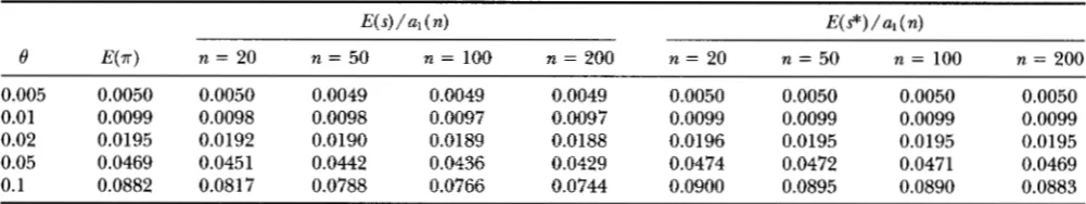
TABLE 1

E(.rr), E ( s ) / a l ( n ) and E(s*)/a,(n) under Jukes and Cantor's model of mutation without rate variation

E ( s ) / a l ( n )

8 E(.rr) n = 20 n = 50 n = 100 n = 200

0.005 0.0050 0.0050 0.0049 0.0049 0.0049 0.01 0.0099 0.0098 0.0098 0.0097 0.0097 0.02 0.0195 0.0192 0.0190 0.0189 0.0188 0.05 0.0469 0.0451 0.0442 0.0436 0.0429

0.1 0.0882 0.0817 0.0788 0.0766 0.0744

E(s*)/al(n)

n = 20 n = 50 n = 100 n = 200

0.0050 0.0050 0.0050 0.0050 0.0099 0.0099 0.0099 0.0099 0.0196 0.0195 0.0195 0.0195 0.0474 0.0472 0.0471 0.0469 0.0900 0.0895 0.0890 0.0883

E(.rr), E ( s ) / a l ( n) and E(s*)/ul ( n ) were obtained from Equations 8, 6 and 15, respectively.

( KIMURA 1968b)

.

Suppose now that n DNA sequences

are randomly sampled from the population. Using the Ewens sampling theory ( EWENS 1972), the probability

(p,

) that a particular site in the sample is exclusively occupied by nucleotide i is given by

Then, the expectation of s is given by

4

E ( s ) = 1 -

pi

= 1 - 4pi, ( 6 )

i= 1

which is approximately given by

where cl ( n ) is given by cl ( n ) = 4al ( n ) / 3 -

5%

( n )

/

{ 3 a l ( n ) ] , al(n) isgiven by ( 2 ) and % ( n ) isgiven by

r

Note that al ( n ) = - S i 2 ' / Si" and @ ( n ) =

Si3'

/

Si", where S;' is the Stirling number of the first kind.

The expectation of

..-

can be obtained by substituting n = 2 into ( 6 ) , and we have

e

1

+

4 e / 3 '

E ( . . - ) =

which agrees with Equation 15 of TAJIMA (1983). Nu- merical examples of E ( ..-) and E ( s)

/

al ( n ) are given in Table 1 since

..-

and s/ al ( n ) are used to estimate 6

under the infinite site model. This table shows that

..-

and s/ al ( n ) give underestimates of 8, that the underes- timation is substantial only when 0 is large, and that the degree of underestimation is larger for s/ al ( n ) than for x. It is also noted that the bias of S / al ( n )

increases as the sample size ( n ) increases. This is be-

cause, as n increases, the probability that more than one mutation occurred in each site among a sample of n sequences also increases. Equations 8 and 6b suggest that 0 can be estimated by

e =

..-

( 9 )

1 - 4..-/3 '

e =

S

(10)

We can estimate

6

from the minimum number of mutations per site ( s * )

.

Let

p,

be the probability that a particular site is exclusively occupied by nucleotides

i

and/ or j , and pyk be the probability that a particular site is exclusively occupied by nucleotides i , j and/or k . Using the same method as we obtained

(5)

,

we obtain

(11)

a l ( n ) - c1(n)s

r ( 4 e / 3 ) r ( z e / 3

+

n ) r ( 4 8 / 3

+

n ) r ( z e / 3 )

'

pij

=

Denote the probability that a particular site is occupied by i types of nucleotide in a sample of n DNA sequences by

qt

and the estimate of

q,

by

g j .

For example, if we have the following five DNA sequences with a length of 20 nucleotides where dash ( - ) indicates the same nucleotide as in the first sequence listed, we have ql =

12

/20, 4 2 = 5/20, 43 = '/20 and 9 4 = '/20.

When a site is occupied by i types of nucleotide in the sample, it is certain that at least i - 1 mutations oc- curred in this site. Therefore, the minimum number of

mutations per site can be estimated by

s* =

&

+

2@3

+

344. (14)

In the above example, we have s* = 5/20

+

2

X 2/20

+

3 X 1/20 = 12/20 = 0.6. It should be noted that s* is the

same as sin the infinite site model, but usually different in the finite site model since s = @

+

+

q4.

From

(13) the expectation of s* can be given by

E ( s * ) = %

+

2qs

+

3q4 = 3 - 4ptjk, (15)

which is approximately given by

w h e r e @ ( % ) = 4 a l ( n ) / 3 - 7 ~ ( n ) / { 3 a l ( n ) ) . N u m e r -

ical examples of E ( s* )

/

al

( n) are also shown in Table

1, which indicate that s*/ a1 ( n ) gives slightly better estimates of

0

than does s/ al ( n )

.

Equation 15a sug- gests that 0 can be estimated by

S*

e =

(16)

a l ( n ) - c z ( n ) s * .

Under the infinite site model, the expected number of nucleotides whose frequency is i/ n per site is given by

f R ( i ) =

0

(t

7

+

-

n!i)

( TAJIMA 1989a), which can be used to identify the pat- tern of DNA polymorphism. Under the present model, it is given by

which can be approximately given by

f n ( i )

=

0 { l / i + l / ( n - 2 ) )

1 + { 4 a l ( n ) / 3 - a l ( n - i ) - a l ( i ) / 3 ] 0 '

(18a)

A comparison between (

17)

and ( 18) indicates that

fn

( i) under the present model is not very different from that of the infinite site model even if 8 is quite large except when i/ n is close to 1.

Jukes and Cantor's model of mutation with rate varia- tion: It has been shown by several authors (e.g., GOLD

ING 1983; WAKELEY 1993) that neutral mutation rates are approximately gamma distributed among sites.

TABLE 2

E(.sr), E ( s ) / a , ( n ) and E(s*)/a,(n) under Jukes and Cantor's model of mutation with rate variation

0.005 0.0047 0.01 0.0087 0.02 0.0155

0.005 0.0048 0.01 0.0093 0.02 0.0172

0.005 0.0049

0.01 0.0096

0.02 0.0185

0.005 0.0049 0.01 0.0097 0.02 0.0190

(A) (Y = 0.1

0.0043 0.0076 0.0123

(B) a = 0.2

0.0046 0.0085 0.0149

(C) (Y = 0.5

0.0048 0.0092 0.0171

(D) (Y = 1

0.0049 0.0095 0.0180

0.0047 0.0088 0.0157

0.0048 0.0093 0.01 74

0.0049 0.0096 0.0186

0.0049 0.0098 0.0191

E(.rr), E ( s ) / q ( n ) and E ( s * ) / a , ( n ) were obtained from for- mulas 22, 21 and 23, respectively, where n = 100 is assumed.

Here, we assume that

0

follows the following gamma distribution:

where a = { E ( 0 ) 1 2 / V ( 0 ) ,

0

= a / E ( 0 ) and E ( 0 ) is the expectation of 0, i.e., E (

0 )

= Bg(

0 )

d8. Note that the smaller (Y is, more the mutation rate varies among

sites. Then, using ( 6 ) , the expectation of the propor- tion of segregating site is given by

E ( s ) =

[

( 1 - 4P*)g(d)d8. (20)

Using ( 6a)

,

E ( s) is approximately given by

Substituting n =

2

into (21 ) , we have

E ( T )

=

E ( 0 )

1

+

4(a

+

l ) E ( 0 ) / ( 3 a )

( 2 2 )

In the same way, the expectation of the minimum num- ber of mutations per site can be obtained, which is approximately given by

1460 F. Tajima

E ( s)

/

al ( n ) and E ( s * )

/

al ( n) are given for n = 100. We can see from this table that the effect of rate varia- tion is substantial when

a

is small ( a

<

1 ) even if E ( 8 )

is as small as 0.005. The effect is stronger on E ( s) than

on

E ( n )

and E ( s * ) . Formulas

( 2 2 ) , ( 2 1 )

and (23)

suggest that we can estimate 8 by

S

d = (25)

a l ( n ) - s ( n ) ( a

+

l ) s / a '

8 = S *

a l ( n ) - s ( n ) ( a

+

l ) s * / a f (26)

if a is known. Although we can also estimate a from these formulas, the accuracy of the estimate might be very low since the variances of s and n are too large to estimate an additional parameter ( WAITERSON 1975; TAJIMA 1983).

Equal-input model of mutation without rate varia- tion: Here, we assume that the mutation rate to nucleo- tide i from any of the other three nucleotides is the same (FELSENSTEIN 1981; TAJIMA and NEI 1982). Namely, when uli is the mutation rate per generation from nucleotide j to nucleotide i, we assume ult = ui

for j f i. Under this model, the mutation rate per generation from nucleotide i to any of the other three nucleotides is XJ+iuj and the expected frequency of nu- cleotide i is given by

(27)

( TAJIMA and NEI 1984). Then, the expected mutation rate per site per generation can be given by

4 4

u = y j uq = hl uj, (28)

z=1 ~ # i i= 1

where hl = 1 - X$=,yf. Following KIMURA (1968b), the probability distribution of the frequency of nucleotide

i, xi, is given by

x (1 - ( 1 - Y z ) O / + 1 _Xi YP/+l ₍₂₉₎

since 4Nut = y i d / h l and 4N Xl++uj = (1 - y i ) O / h l , where 8 = 47%. Using the Ewens sampling theory ( EWENS 19'72), the probability

( p i

) that a particular site in the sample is exclusively occupied by nucleotide

i is given by

Then, the expectation of s is given by

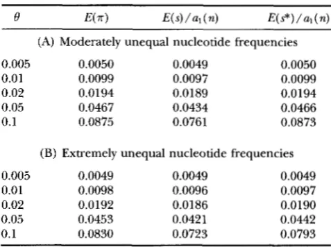
TABLE 3

E(m), E ( s ) / a l ( n ) and E(s*)/a,(n) under the equal-input model of mutation without rate variation

I 9 E(.rr) E ( s ) / a 1 ( n ) W s * ) / a , ( n )

(A) Moderately unequal nucleotide frequencies

0.005 0.0050 0.0049 0.0050 0.01 0.0099 0.0097 0.0099 0.02 0.0194 0.0189 0.0194 0.05 0.0467 0.0434 0.0466 0.1 0.0875 0.0761 0.0873

(B) Extremely unequal nucleotide frequencies

0.005 0.0049 0.0049 0.0049 0.01 0.0098 0.0096 0.0097 0.02 0.0192 0.0186 0.0190 0.05 0.0453 0.0421 0.0442 0.1 0.0830 0.0723 0.0793

E(.rr), E ( s ) / a l ( n ) and E ( s * ) / a l ( n ) were obtained from Equations 32, 31 and 35, respectively, where n = 100 is as- sumed. Moderately unequal nucleotide frequencies assume

yl = O.l,% = 0.3, y3 = 0.4 and y4 = 0.2, and extremely unequal nucleotide frequencies assume yl = 0.025, y2 = 0.225, y3 =

0.675 and p = 0.075.

4

E ( s ) = 1 -

c

pz,

(31) i= 1

which is approximately given by

where

h2

= 1 -

Xf=lyS.

On the other hand, the expecta-

tion of n is given by

8

E ( n ) =

1

+

d / h l .

(34)

Then, the expectation of s* is given by

which is approximately given by

100 is assumed. A comparison between Tables 1 and 3

shows that E ( 7 r ) and E ( s) under this model are not very different from those under Jukes and Cantor’s model even when the nucleotide frequency deviates substantially from equality, whereas E ( s*) under this model is quite different from that under Jukes and Can- tor’s model when the nucleotide frequency deviates substantially from equality. Using (31a), ( 3 2 ) and

(35a), we can estimate 8 by

In these equations,

h,

and

&

can be estimated by

h,

=

1 -

E

jp and j& = 1 -

E

9:

,

where j t is the observed frequency of nucleotide i.

Under this model the expected number of nucleo- tides whose frequency is i/ n per site is given by

(39)

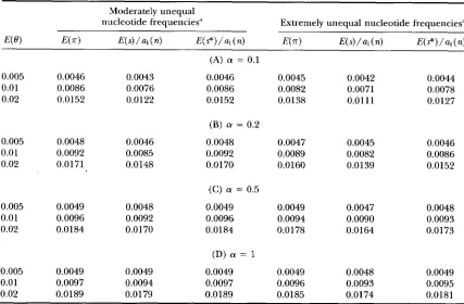
Equal-input model of mutation with rate varia- tion: When 8 follows the gamma distribution ( 19)

,

the expectations of x, s and s* are approximately given by

( 4 2 )

Numerical examples are shown in Table 4. It can be seen from this table that the effect of rate variation is substantial when a is small ( a

<

1 ) even if E ( 8 ) is as small as 0.005 and that the effect is stronger on E ( s)

than on E (

x).

The above formulas suggest that, if a is known, 0 can be estimated by

8 = 7r (43)

1 - ( a

+

1 ) 7 r / ( h 1 a ) ’

S *

Kimura’s model of mutation without rate varia- tion: We now assume that the rate of transitional muta- tion is different from that of transversional mutation ( KIMURA 1980). Namely, we assume uI2 = uYl = u34 =

u43 = cru and ~ 1 3 = u14 = uZ3 = y4 = usl = u32 = 2141 =

~ 4 2 = ( w / 2 ) u and cr

+

w = 1, where uq is the mutation

rate per site per generation from nucleotide i to nucleo- tide j , u is the total mutation rate per site per genera- tion, cr is the proportion of transitional mutation, and

w is the proportion of transversional mutation. Unlike the previous models, under this model we cannot ob- tain the expectations of s and s* since we cannot obtain

p,

.

We can, however, obtain

p,

as follows. The mutation rate from A or G to C or T is 2wu, and the mutation rate from C or T to A or G is also 2wu. Therefore,

p1~

( = $44

1

is given by

Since the mutation rate from A or C to G or T and that from G or T to A or C are ( a

+

w / 2 ) u ,

PIS

( = P I 4 =

p2, =

h4)

is given by

Denote the probability that a particular site is occupied by ( A and G ) or ( C and T ) in a sample of n DNA sequences by q., and the probability of having ( A and C ) , (A and T ) , ( G and C ) or ( G and T ) by 4.. In other words, g2 is divided into the transitional part (4.)

and the transversional part (4.). In the previous exam- ple, the estimates of q. and q. are 4/20 and respec-

tively. If we denote

qa

and

qb

by

1462 _F. Tajima

TABLE 4

E(m), E ( s ) / a ~ ( n ) and E((s*)/a,(n) under the equal-input model of mutation with rate variation

Moderately unequal

nucleotide frequencies" Extremely unequal nucleotide frequencies"

E ( @ ) E(-ir) E(s)/a1(n) E ( ? ) / u I ( ~ ) E(.rr) E ( s ) / a , ( n ) E(s*)/al(n)

(A) (Y = 0.1

0.005 0.0046 0.0043 0.0046 0.0045 0.0042 0.0044 0.01 0.0086 0.0076 0.0086 0.0082 0.0071 0.0078 0.02 0.0152 0.0122 0.0152 0.0138 0.01 11 0.0127

(B) (Y = 0.2

0.005 0.0048 0.0046 0.0048 0.0047 0.0045 0.0046 0.01 0.0092 0.0085 0.0092 0.0089 0.0082 0.0086 0.02 0.0171 0.0148 0.0170 0.0160 0.0139 0.0152

(C) (Y = 0.5

0.005 0.0049 0.0048 0.0049 0.0049 0.0047 0.0048 0.01 0.0096 0.0092 0.0096 0.0094 0.0090 0.0093 0.02 0.0184 0.0170 0.0184 0.0178 0.0164 0.0173

(D) a = 1

0.005 0.0049 0.0049 0.0049 0.0049 0.0048 0.0049 0.01 0.0097 0.0094 0.0097 0.0096 0.0093 0.0095 0.02 0.0189 0.0179 0.0189 0.0185 0.0174 0.0181

E(.rr), E ( s ) / a , ( n ) and E ( s * ) / a l ( n ) were obtained from formulas 40, 41 and 42, respectively, where n = 100

a See Table 3.

is assumed.

4. = 1 - 2p12 and q b = 1 -

2p13,

(49)

which are approximately given by

4.

-

a1 ( n )

we

( U

+

4 2 1 0

1

+

a ( n ) w e

and 4 0

=

1

+

c 3 ( n ) (a

+

w / 2 ) e 7

(50)

where g ( n ) = 2al ( n ) - 3a, ( n )

/

al ( n )

.

These formu-

las suggest that 8, w and a can be estimated by

e =

4

+

i b , (51a)

( j =

4

2 { a l ( n ) - c3(n)421 a l ( n ) - C 3 ( n ) g b

1al(n) - C3(n)(i,Ie

and 8 = 1 - G. (51b)

Let us now denote the average numbers of painvise transitional and transversional differences per nucleo- tide site by ns and T,, respectively. When n = 2, we have qa = E (

x,)

and q b = E ( T ~ )

+ E (

T,,) / 2 since E ( ns) =

q,, and E ( T , ) = q,,. From ( 4 9 ) , we have

It is noted that E ( n ) = 8 / ( 1

+

40/3) if there is no transition bias (ie., w = * / 3 ) . Numerical examples are shown in Table 5, which indicate that n underestimates 0 when

8

is very large and that the amount of underesti- mation is the slightest when there is no transition bias. Equations 52a and 52b indicate that we can estimate

8, w and u by

e =

x,

+

7FJ2

+

T U

1 - (2n,

+

n,) 2 ( 1 - 2n,)

,

(54a)

Lj= T U

( 1 - 27r,)B

and 6 = 1 - G. (54b)

Kimura's model of mutation with rate variation: We again assume that 8 follows the gamma distribution ( 1 9 ) . In the same way as before, we can obtain the expectation of q. and q b , which are approximately given bY

Amount of DNA Polymorphism

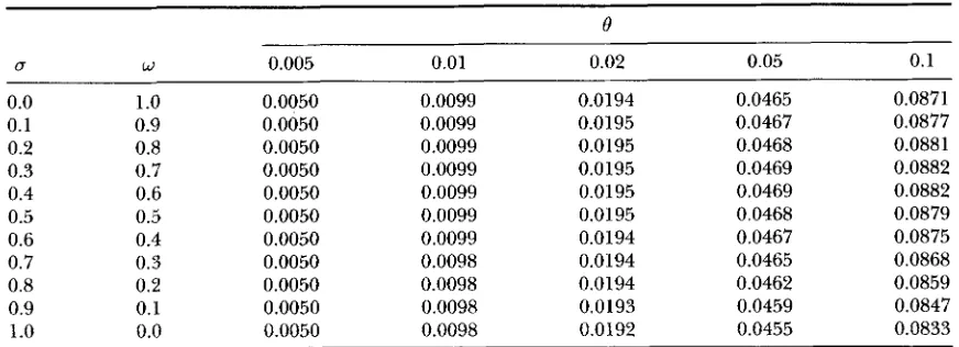
TABLE 5

E ( m ) under Kimura’s model of mutation without rate variation

e

U W 0.005 0.01 0.02 0.05 0.1

0.0 1

.o

0.0050 0.0099 0.0194 0.0465 0.0871

0.1 0.9 0.0050 0.0099 0.0195 0.0467 0.0877

0.2 0.8 0.0050 0.0099 0.0195 0.0468 0.0881

0.3 0.7 0.0050 0.0099 0.0195 0.0469 0.0882

0.4 0.6 0.0050 0.0099 0.0195 0.0469 0.0882

0.5 0.5 0.0050 0.0099 0.0195 0.0468 0.0879

0.6 0.4 0.0050 0.0099 0.0194 0.0467 0.0875

0.7 0.3 0.0050 0.0098 0.0194 0.0465 0.0868

0.8 0.2 0.0050 0.0098 0.0194 0.0462 0.0859

0.9 0.1 0.0050 0.0098 0.0193 0.0459 0.0847

1

.o

0.0 0.0050 0.0098 0.0192 0.0455 0.0833

E(T) was obtained from Equation 53.

E ( T , )

+

E ( 7 r u ) / 2 ( a

+

w / 2 ) 8

1

+

( a

+

1 ) ( 2 0

+

w ) 8 / a

’

(57b)

the expectation of 7r is approximately given by

E(.rr)

(1

+

3 ( a

+

1 ) ( 1 -

W / 2 ) w e / a ~ ~

( 1

+

2 ( a

+

l ) w 8 / a } { l

+

( a

+

1 ) ( 2 - w ) 8 / a )

c

(58)

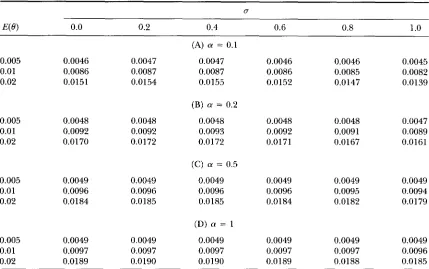
Numerical examples are shown in Table 6, which indi- cate that the effect of rate variation on 7r is substantial

even when E ( 8 ) is as small as 0.005 and that the effect increases as the transition

/

transversion bias increases from a = Formulas 57a and 57b suggest that if CY is known, 8, w and a can be estimated by

O =

T s

+

7 r J 2

1 - ( a

+

1)(27rs

+

7r,)/a

+

T U

2 ( 1 - 2 ( a

+

l)7ru/a)

9 (59a)

Lj= T”

( 1 - 2 ( a

+

l ) T , / a ) e and b = 1 - G . (59b)

DISCUSSION

The infinite site model is one of the fundamental models for molecular population genetics. In fact, a large number of important theoretical studies were based on this model. This model, however, is not always applicable. As shown in this paper, when the rate of mutation vanes substantially among sites, the amount of DNA polymorphism estimated by using this model might be underestimated. For example, the amount of underestimation might be substantial in the case of the control region of human mitochondrial DNA.

HORAI

and coworkers examined the 482-bp sequences in the control region from Africans, Europeans, Asians and Native Americans ( HORAI and HAYASAKA 1990; HORAI et al. 1991,1993). I have analyzed the 250-bp sequences in hypervariable region 1, since an estimate of a is avail- able in this region, i.e., 13 = 0.47 ( WAKELEY 1993). Table

7

shows the estimates of

8,

a and w obtained from the infinite site model, Jukes and Cantor’s model, the equal-input model and Kimura’s model by using n =

1464 F. Tajima

TABLE 6

E(m) under Kimura’s model of mutation with rate variation

U

E ( @ 0.0 0.2 0.4 0.6 0.8 1

.o

(A) a = 0.1

0.0047 0.0087 0.0155 0.005 0.01 0.02 0.0046 0.0086 0.0151 0.0047 0.0087 0.0154 0.0046 0.0086 0.0152 0.0046 0.0085 0.0147 0.0045 0.0082 0.0139

(B) a = 0.2

0.0048 0.0093 0.01 72 0.005 0.01 0.02 0.0048 0.0092 0.0170 0.0048 0.0092 0.0172 0.0048 0.0092 0.0171 0.0048 0.0091 0.0167 0.0047 0.0089 0.0161

(C) a = 0.5

0.0049 0.0096 0.0185 0.005 0.01 0.02 0.0049 0.0096 0.0184 0.0049 0.0096 0.0185 0.0049 0.0096 0.0184 0.0049 0.0095 0.0182 0.0049 0.0094 0.0179

(D) a = 1

0.0049 0.0097 0.0190 0.005 0.01 0.02 0.0049 0.0097 0.0189 0.0049 0.0097 0.0190 0.0049 0.0097 0.0189 0.0049 0.0097 0.0188 0.0049 0.0096 0.0185

E(n) was obtained from (58).

the estimates obtained from s and s*, probably because these mutation models do not fit the data. Since the transitional mutation rate is substantially higher than transversional mutation rate in mammalian mitochon- drial DNA sequences, Kimura’s model might be more appropriate. It is also shown in the table that in the case of Kimura’s model the estimate of 6’ with rate varia- tion is quite different from that without rate variation. Namely the value with rate variation is 2.5 times larger than that without rate variation.

8

=

0.2 may not be

unreasonable, since 6’ is determined by the recent popu- lation size more strongly than by the ancient population size (TAJIMA 1989b) and since the human population might have increased (MERRIWETHER et al. 1991; ROC? ERS and HARPENDING 1992).

Recently, several methods for estimating 0, including

Fu (1994a,b) and KUHNER et al. (1995), have been proposed. Fu’s methods, however, assume that there is no rate variation among nucleotide sites, so that they may give an underestimate of 6’ when the mutation rate

TABLE 7

Estimates of 8, u and (o in the 250-bp hypervariable control region of human mitochondrial DNA

~ Model

~~

Measure used

e

6 L3 Formula

~ ~

Infinite site model S 0.0685 3b

Jukes and Cantor’s model

Without rate variation S 0.0874

S* 0.0794

With rate variation S 0.2113

S* 0.1017

10 16 25 26 Equal-input model

Without rate variation 7 0.0880 37

s* 0.081 1 38

With rate variation S 0.2231 44

sy 0.1110 45

Without rate variation da, q b 0.0897 0.9298 0.0702 51

With rate variation

_da,

d b 0.2283 0.971 1 0.0289 56

Kimura’s model

~

varies among sites. Since we do not know the effect of rate variation on his methods, we must be careful when the rate varies among sites substantially. On the other

hand, KUHNER et aL’s method can deal with rate varia-

tion by using a mutation rate category approach, al-

though this approach has not been extensively tested.

BERTORELLE and SLATKIN ( 1995 ) clearly indicate that

the test of neutrality proposed by TAJIMA ( 1989a) might

not be appropriate if the mutation rate varies among sites substantially. This is because Tajima’s D statistic is

based on the infinite site model. FU and LI’S (1993)

test also has the same problem. The variances of 7r and

s and the covariance between IT and s remain to be

solved under the finite site models with rate variation. If we know them, we will be able to alleviate this problem.

I thank an anonymous reviewer for many valuable suggestions and comments for improving the presentation. This work was supported in part by a grant-in-aid from the Ministry of Education, Science, Sports and Culture of Japan.

LITERATURE CITED

BERTORELLE, G., and M. SLATKIN, 1995 The number of segregating sites in expanding human populations, with implications of esti-

mates of demographic parameters. Mol. Biol. Evol. 12: 887-892. EWENS, W. J., 1972 The sampling theory of selectively neutral alleles.

Theor. Popul. Biol. 3: 87-112.

FELSENSTEIN, J., 1981 Evolutionary trees from DNA sequences: a maximum likelihood approach. J. Mol. Evol. 17: 368-376.

Fu, Y.-X., 1994a A phylogenetic estimator of effective population size or mutation rate. Genetics 136: 685-692.

Fu, Y.-X., 1994b Estimating effective population size or mutation rate using the frequencies of mutations of various classes in a sample of DNA sequences. Genetics 1 3 8 1375-1386.

Fu, Y.-X., and W.-H. LI, 1993 Statistical tests of neutrality of muta- tions. Genetics 133: 693-709.

GOLDING, G. B., 1983 Estimates of DNA and protein sequence diver- gence: an examination of some assumptions. Mol. Biol. Evol. 1:

HOW, S., and K. HAYASAKA, 1990 Intraspecific nucleotide sequence differences in the major noncoding region of human mitochon- drial DNA. Am. J. Hum. Genet. 46: 828-842.

HOW, S., R. KONDO, K. MURAYAMA, S. HAYASHI, H. KOIKE et al., 1991 Phylogenetic f i l i a t i o n of ancient and contemporary humans 125-142.

inferred from mitochondrial DNA. Phil. Trans. R. SOC. Lond. B

HOW, S., R. KONDO, Y. NAKAGAWA-HATTOM, S. HAYASHI, S. SONODA

et al., 1993 Peopling of the Americas, founded by four major lineages of mitochondrial DNA. Mol. Biol. Evol. 10: 23-47. JUICES, T. H., and C. R. CANTOR, 1969 Evolution of protein mole-

cules, pp. 21-132 in Mammalian Protein Metabolism, edited by H. N. MUNRO. Academic Press, New York.

KIMURA, M., 1968a Evolutionary rate at the molecular level. Nature

KIMURA, M., 1968b Genetic variability maintained in a finite popula- tion due to mutational production of neutral and nearly neutral isoalleles. Genet. Res. 11: 247-269.

KIMURA, M., 1969 The number of heterozygous nucleotide sites maintained in a finite population due to steady flux of mutations. Genetics 61: 893-903.

KIMURA, M., 1980 A simple method for estimating evolutionary rate of base substitutions through comparative studies of nucleotide sequences. J. Mol. Evol. 16: 111-120.

KIMURA, M., 1983 The Neutral Theory of Molecular Evolution. Cam- bridge University Press, Cambridge.

KUHNER, M. IC, J. YAMATO and J. FELSENSTEIN, 1995 Estimating effec- tive population size and mutation rate from sequence data using Metropolis-Hastings sampling. Genetics 140: 1421-1430. MERRIWETHER, D. A., A. G. CLARK, S. W. BALLINGER, T. G . SCHURR,

H. SOOOYALL et aZ., 1991 The structure of human mitochondrial DNA variation. J. Mol. Evol. 33: 543-555.

ROGERS, A,, 1992 Error introduced by the infinite-sites model. Mol. Biol. Evol. 9: 1181-1184.

ROGERS, A. R., and H. HARPENDING, 1992 Population growth makes waves in the distribution of pairwise genetic differences. Mol. Biol. Evol. 9: 552-569.

TAJIMA, F., 1983 Evolutionary relationship of DNA sequences in fi- nite populations. Genetics 105: 437-460.

TAJIMA, F., 1989a Statistical method for testing the neutral mutation hypothesis by DNA polymorphism. Genetics 1 2 3 585-595. TAJIMA, F., 198913 The effect of change in population size on DNA

polymorphism. Genetics 123: 597-601.

TAJIMA, F., and M. NEI, 1982 Biases of the estimates of DNA diver- gence obtained by the restriction enzyme technique. J. Mol. Evol.

TAJIMA, F., and M. NEI, 1984 Estimation of evolutionary distance between nucleotide sequences. Mol. Biol. Evol. 1: 269-285. WAKELEY, J., 1993 Substitution rate variation among sites in hyperva-

riable region 1 of human mitochondrial DNA. J. Mol. Evol. 37:

WATTERSON, G. A., 1975 On the number of segregating sites in genetic models without recombination. Theor. Popul. Biol. 7:

256-276.

3 3 3 409-417.

217: 624-626.

18: 115-120.

613-623.