LONG, DANIEL ESLEY. System Excess Placement for Improving Lifecycle Value. (Under the direction of Dr. Scott Ferguson.)
The objective of this research is understanding, modeling, and evaluating the use of
strategic overdesign (excess) as a method for minimizing the cost of system change to maximize
system lifecycle value. This research is necessary because the design and construction of modern
complex engineered systems is costly, and these systems operate in a context that changes over
time. Reducing (and ideally minimizing) the cost of executing system adaptations is therefore
advantageous. Prior research provides guidance for how system changeability can be supported
by encapsulating functionality within modules, but little research has been dedicated to optimal
design variable (or component sizing) selection to support future system changes. The specific
© Copyright 2020 by Daniel Long
by
Daniel Esley Long
A dissertation submitted to the Graduate Faculty of North Carolina State University
in partial fulfillment of the requirements for the degree of
Doctor of Philosophy
Aerospace Engineering
Raleigh, North Carolina
2020
APPROVED BY:
_______________________________ _______________________________ Dr. Scott Ferguson Dr. Julie Ivy
Committee Chair
ii BIOGRAPHY
Daniel Long is a PhD candidate studying Aerospace Engineering at North Carolina State
University. His research uses data science for studying how system changeability and value may
be improved by including excess in the initially fielded system. Daniel received his B.S. in 2006
from North Carolina State University in Nuclear Engineering and his MS degree in Aerospace
Engineering from North Carolina State University in 2014. Daniel has worked for Progress
Energy as a Fuel Supply and Nuclear Core Design engineer and for NASA Langley as an intern
in the Space Missions Analysis Branch. Daniel has also completed the International Space
iii ACKNOWLEDGMENTS
The author would like to acknowledge support from the American Public Power Association as
part of a Demonstration of Energy and Efficiency Developments Grant, the U.S. Department of
Energy through the Cities Leading through Energy Analysis and Planning Award, and the
Garrett Fellowship.
I would like to thank and to express my most sincere gratitude to my adviser Dr. Scott Ferguson
for his tireless effort in guiding my research, his help trimming and focusing drafts that were
always far too long, and helping me grow as a researcher and engineer. I would not be where I
am today without his help. I would also like to thank the member of my committee Dr. Gregory
Buckner, Dr. Andre Mazzoleni, and Dr. Julie Ivy for both their insightful feedback on my
research and for the roles they have played in teaching and guiding me throughout my academic
career.
I would like to thank my former and current fellow students in the System Design and
Optimization Laboratory. You have each helped me during my time as a student by teaching,
sharing, and supporting me when I needed it.
Finally, I would not be where I am today without the patience, support, and love from friends,
family, and pets. You all kept me going! I am especially for the support from my partner April
Cash who has been patient and supportive when work hours grew long.
iv TABLE OF CONTENTS
LIST OF TABLES ... viii
LIST OF FIGURES ... x
Chapter 1: Introduction ... 1
1.1 Motivation ... 1
1.2 The Phenomenon of Change Propagation... 2
1.3 Design Margin and Excess... 5
1.4 Research Plan Overview ... 6
1.5 Dissertation Outline ... 9
Chapter 2: Background ... 10
2.1 Introduction ... 10
2.2 Engineering Design Process and Engineering Change Context ... 10
2.3 What is Flexibility? ... 11
2.4 What design features add to system flexibility an dhow are those features measured? ... 12
2.5 How can design options be compared to find a “best” one? ... 15
2.6 Component-Level Change-Importance Metrics ... 17
2.6.1 Design for Variety... 17
2.6.2 Change Propagation Method... 19
2.6.3 Change Propagation Index ... 23
2.7 Design Margin and Excess... 25
2.8 Chapter Summary ... 28
Chapter 3: Qualitative Excess Assessment of Two Historical Military Aircraft ... 29
3.1 Introduction ... 29
3.2 Method for Case Study ... 30
3.3 The B-52 Stratofortress ... 31
3.3.1 Historical Context ... 31
3.3.2 Lifecycle Analysis ... 33
3.3.2.1 Surface to Air Missiles (SAMs) ... 33
3.3.2.2 Change in Operational Altitude ... 33
3.3.2.3 Survivability Enhancements ... 34
3.3.2.4 Standoff Weapons ... 35
3.3.2.5 Conventional Weapons Modifications ... 36
3.3.2.6 Modern Electronics Integration ... 37
3.3.3 B-52 Summary ... 38
3.4 The F/A-18 Hornet ... 38
3.4.1 Historical Context ... 38
3.4.2 Lifecycle Analysis ... 40
3.4.3 Symptoms of Insufficient Excess... 42
3.4.3.1 Range/Payload ... 42
3.4.3.2 Internal System’s Growth ... 44
3.4.3.3 Payload Recovery ... 45
v
3.5 Discussion ... 47
3.6 Chapter Summary ... 51
Chapter 4: Excess in Gaming PCs ... 53
4.1 Introduction ... 53
4.1.1 A Brief Discussion of Gaming Systems – Computers and Consoles ... 54
4.1.2 Chapter Outline ... 57
4.2 Data Collection and Console Comparison ... 57
4.2.1 Data Collection ... 58
4.2.1.1 Game Requirements ... 58
4.2.1.2 Recommended/Suggested Computer Builds... 59
4.2.1.3 Desktop Hardware Performance Specifications ... 61
4.2.1.4 Console Hardware ... 61
4.2.2 Data Processing ... 62
4.3 Console and Desktop Comparison ... 63
4.4 Desktop Excess Assessment ... 68
4.4.1 Component Specification Comparisons ... 68
4.4.2 SPM Calculation ... 69
4.4.3 Desktop Performance Using the SPM Metric ... 69
4.4.4 Assessing the Utility of a Desktop Gaming Computer ... 72
4.5 Strategic Excess at Component Level ... 73
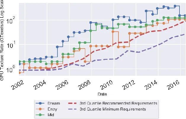
4.6 Temporal Comparison of Hardware Performance vs Requirements ... 79
4.7 Discussion ... 82
4.8 Chapter Summary ... 87
Chapter 5: Dynamic Change Probabilities and their Role in Change Propagation ... 90
5.1 Introduction ... 90
5.2 Background ... 92
5.3 Method for Studying DCP ... 93
5.3.1 Changed Components Identification ... 95
5.3.2 Updating Direct Likelihood Probabilities ... 97
5.3.3 CPC Score and Sample Trajectory Evaluation ... 99
5.4 System-Level Study of DCP and System Architecture ... 102
5.4.1 Study of System Architectures from the Literature ... 103
5.4.1.1 Experimental Setup ... 103
5.4.1.2 Results ... 103
5.4.2 Study of Synthetically Generated System Architectures ... 106
5.4.2.1 Algorithm for Generating Synthetic System Architectures ... 106
5.4.2.2 Experimental Setup ... 108
5.4.2.3 Results ... 110
5.5 Component-level study of DCP and system architecture ... 112
5.5.1 Increases in Component-Level propagation between initial and terminal configurations ... 113
5.5.1.1 Experimental Setup ... 113
5.5.1.2 Results ... 114
vi
5.5.2.1 Experimental Setup ... 119
5.5.2.2 Results ... 119
5.6 Discussion ... 121
Chapter 6: Excess Based Change Propagation ... 125
6.1 Introduction ... 125
6.2 Background ... 128
6.2.1 Real Options Analysis... 128
6.2.2 Model-Based Systems Engineering ... 129
6.2.3 What is missing and what can we learn? ... 129
6.3 Overview of The Approach ... 131
6.4 Creating object-oriented models ... 132
6.4.1 System Configuration ... 133
6.4.2 System Design ... 134
6.4.2.1 Flow Tracking via Computation Network ... 134
6.4.2.2 Requirements Tracking ... 136
6.4.3 Exogenous Variables ... 137
6.4.3.1 Technology Limits ... 137
6.4.3.2 Environmental and Systems of Systems Variables ... 139
6.4.4 System Attributes, Costs, and Value ... 140
6.4.4.1 Recurring Costs ... 141
6.4.4.2 Non-Recurring Costs ... 141
6.5 Discrete-Time Simulation ... 141
6.6 Procedure for Modeling System Change ... 142
6.6.1 Initiate Change at Chosen Node ... 143
6.6.2 Generate Change Pathways... 143
6.6.3 Evaluation of Change Costs ... 145
6.6.4 System Performance ... 145
6.7 Desktop computer example study ... 135
6.7.1 Common System Model ... 146
6.7.2 Value Assessment and Change Propagation ... 149
6.7.3 Experiment One – Value of Excess in a Component ... 150
6.7.3.1 Setup ... 150
6.7.3.2 Results ... 151
6.7.4 Experiment Two - Value of Excess in a System ... 152
6.7.4.1 Setup ... 152
6.7.4.2 Results ... 152
6.8 Chapter Summary ... 158
Chapter 7: Conclusions and Future Work ... 160
7.1 Research Summary ... 160
7.2 Discussion of Research Questions ... 160
7.3 Future Research ... 165
7.3.1 Excess in Practice Case Study ... 166
7.3.2 Value and Risk Modeling ... 167
vii
7.3.4 The Coupled System/Strategy Problem ... 170
APPENDICES ... 186
Appendix 1: Remaining System Direct Likelihood DSMs ... 187
Appendix 2: System CPC by Generation Figures... 188
Appendix 3: Component CPC Figures ... 189
viii LIST OF TABLES
Table 2.1 DSM Example showing calculation of coupling indices ... 18
Table 2.2 Results from application of DfV on a water cooler with three metrics and
anticipated non-recurring engineering costs incurred by redesign ... 19
Table 2.3 Direct likelihood matrix containing the probability that one component directly changes another ... 20
Table 2.4 Combined likelihood matrix resulting from the summation of all pathways
between each pair of components ... 22
Table 2.5 Types of excess capability and their associated parameters ... 27
Table 3.1 Comparison of Select Attributes for B-52 models ... 32
Table 3.2 A comparison select parameters between operational US strategic bombers
showing parameter excess with respect to the requirements of newer aircraft ... 32
Table 3.3 Comparison of Select Attributes of F/A-18 Models ... 41
Table 3.4 Proposed F/A-18 modifications with associated weight and volume changes
showing miniaturization required to support desired modifications ... 45
Table 3.5 Weight Increase of Precision Munitions ... 46
Table 3.6 Comparison of Select System Attributes ... 51
Table 4.1 Abbreviated example of data captured for a videogame demonstrating how
hardware/software requirements may be communicated ... 59
Table 4.2 A recommended Mid-level build from 2008 with components and corresponding then-current prices from PC Gamer ... 61
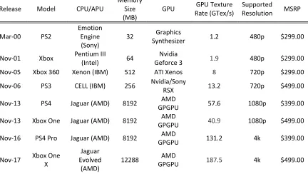
Table 4.3 Specifications for Microsoft and Sony console releases from 2000 to 2019 ... 62
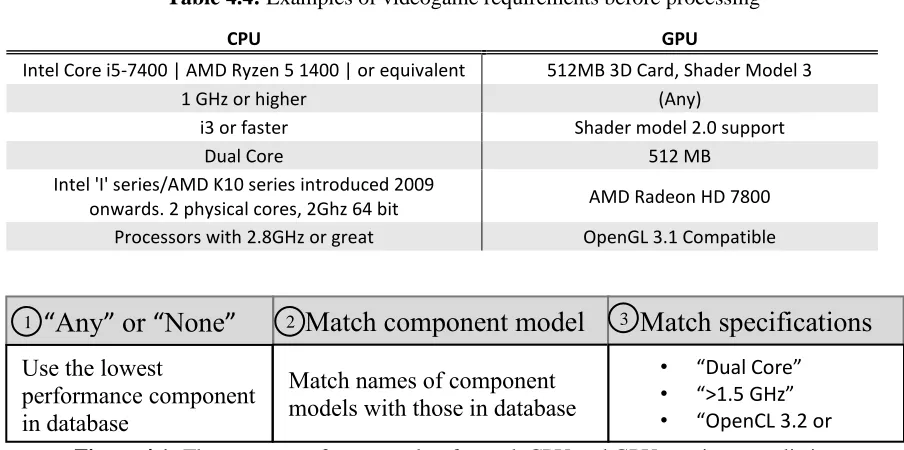
Table 4.4 Examples of videogame requirements before processing ... 63
Table 4.5 Performance measures used to compare a desktop computer to game
requirements ... 69
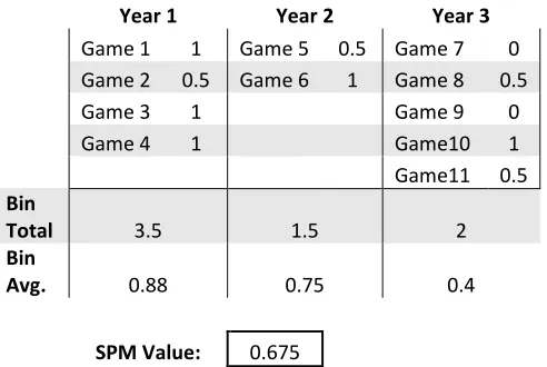
Table 4.6 Notional SPM calculation for three-year period ... 71
ix Table 5.1 Test system properties and references ... 103
Table 5.2 DCP metrics for tested systems in order of increasing number of edges ... 104
Table 5.3 Initial weight vs probability of component selection after being chosen for edge showing the influence that γ has on hub creation ... 109
Table 5.4 Numerical results from architecture testing ... 112
Table 5.5 Relative cCPC increase and percent change in sCPC contribution between
initial and terminal DSMs for the UGV ... 117
Table 5.6 Pearson correlation coefficients showing which network properties affect cCPC and contributions to sCPC ... 117
Table 5.7 Reductions levels applied to dependency values ... 119
Table 5.8 Component-wise Pearson correlation coefficients of metric vs excess addition for the UGV ... 121
Table 6.1 Example RAM Component Information ... 148
Table 6.2 System components for the three initial system configurations. Only the Entry Level is used in the first experiment ... 148
Table 6.3 Exogenous variable parameters and their levels ... 152
Table 6.4 Mean lifecycle value of all simulated systems for simulations using tested
x LIST OF FIGURES
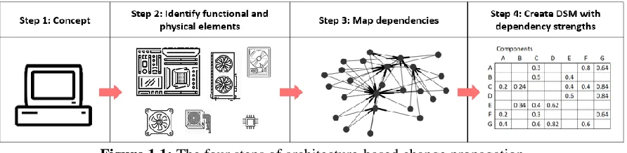
Figure 1.1 The four steps of architecture-based change propagation ... 3
Figure 1.2 Notional example showing relationships between system parameters, margin, requirements, and excess ... 6
Figure 2.1 UGVs with different market segments displaying commonality and differentiation ... 14
Figure 2.2 A Decision Based Design Approach ... 15
Figure 2.3 Change propagation pathway tree from initiator (a) to the target component (b) .... 21
Figure 2.4 Probability calculation using And and Or operations ... 22
Figure 2.5 A comparison of notional change processes with increasing number of high CPI components ... 24
Figure 2.6 A heating element example of a component flow model ... 28
Figure 3.1 Ordinance comparison for modern US Bombers ... 37
Figure 3.2 Visual Comparison of F/A-18 Models ... 41
Figure 3.3 F/A-18 C Fuel Storage ... 44
Figure 3.4 F/A-18 E Fuel Storage ... 44
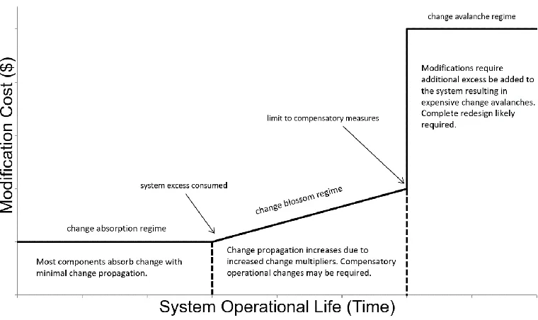
Figure 3.5 Notional chart showing how the consumption of excess increases costs of modifications until the system must be redesigned ... 48
Figure 4.1 The sequence of text searches for each CPU and GPU requirements listing ... 63
Figure 4.2 Comparison of console and computer GPUs performance showing computers’ more frequent releases versus longer Xbox and PlayStation generations ... 66
Figure 4.3 Comparison of console and minimum game requirements for GPUs showing console showing consoles capable of supporting most game GPU minimum requirements for the entire generation and most recommended game setting for about half the generation ... 67
xi Figure 4.5 Suggested computer build SPM values over time demonstrating more excess
provides robustness vs requirements changes and a trend of increased game
requirements lag in the latter portion of the study period ... 72
Figure 4.6 Utility using a ratio of SPM to cost demonstrating the entry level system generally outperforming Mid and Dream computers ... 74
Figure 4.7 Build utility using only top 20 performance games in each year demonstrating Mid computer generally having the highest utility ... 76
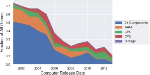
Figure 4.8 Fraction of unsatisfied game requirements per component by computer type and year demonstrating that 2+ component failures are the most common and that the total un-runnable fraction decreases over time for all systems ... 78
Figure 4.9 Fraction of games made runnable by adding strategic excess by component and computer ... 79
Figure 4.10 Mean and 95% percentile of GPU hardware releases and game requirements binned quarterly demonstrating an exponential increase for both ... 80
Figure 4.11 Mean and 95% percentile of CPU hardware releases and game requirements binned annually demonstrating an exponential rate of increase for both requirements and hardware with game requirements leveling off around 2013 ... 81
Figure 4.12 Comparison of levels of CPU performance and ability to satisfy median game requirement demonstrating between 1st and 2nd quartile generally meeting 6-year lifecycle target ... 82
Figure 4.13 Comparison of levels of GPU performance and ability to satisfy median game requirement demonstrating between 75 and 90 percentiles generally meeting 6-year lifecycle target ... 82
Figure 5.1 Method Pseudo-Code overview ... 94
Figure 5.2 Propagation simulation pseudocode ... 96
Figure 5.3 Propagation probability modification pseudocode ... 98
Figure 5.4 Combined likelihood matrix showing how sCPC and cCPC metrics are calculated ... 100
Figure 5.5 A sample plot of sCPC vs. Generation for n=100 including mean line and both metrics for Helicopter ... 102
xii Figure 5.7 Hairdryer and grill direct likelihood DSMs ... 105
Figure 5.8 Algorithm for network generation ... 108
Figure 5.9 Plots showing the relationships between the number and type of hubs on three chosen properties. Plots indicate that in most cases hubs help to slow increases in propagation probabilities and reduce maximum sCPC ... 111
Figure 5.10 The average cCPC at various generations for the UGV showing pronounced
differences between generation 0 and generation 30 ... 114
Figure 5.11 Chart showing the frequency of component rank from all generations and trials for the UGV ... 118
Figure 5.12 Excess vs Average Generations (higher is better) ... 120
Figure 5.13 Excess vs Slope (lower is better) showing improvement for most components
and significant improvement in some... 120
Figure 6.1 Modified DBD framework adapted from Hazelrigg [28] ... 131
Figure 6.2 System model framework describing the steps and sequencing for how the system model is assembled. The dashed boxes indicate where DBD boxes are embodied ... 133
Figure 6.3 Computation graph showing how values (flows) transfer via edges ... 135
Figure 6.4 Computational graph with attributes and calculations imbedded in a block ... 136
Figure 6.5 Block graph showing how requirements are implemented in the computational graph ... 137
Figure 6.6 Normalized NVIDIA GPU ... 139
Figure 6.7 System model demonstrating how standard interface matching abstracts
geometry detail and how attributes of the external system included ... 140
Figure 6.8 A diagram showing the simulation as divided into epochs separated by rebuilds until termination criteria are reached ... 142
Figure 6.9 Simulation strategy for assessing change propagation and linking it to lifecycle value ... 143
Figure 6.10 Change option example showing the “Add GPU” and “Replace Component”
xiii Figure 6.11 Larger initial power supplies increase component commonality but that
lifecycle value improvement peaks at 750W ... 151
Figure 6.12 System lifecycle value distribution by computer type and scenario (Halving Time, Discount Rate) showing the sensitivity of the outcomes to each category. The halving time and the initial computer appear to have the greatest influence .. 153
Figure 6.13 A comparison of E2 Total Cost and number of common components showing decreasing value ... 155
Figure 6.14 E2 costs vs component instance showing that the type and number of GPU used has the largest impact on system value ... 156
Figure A1.1 Helicopter ... 187
Figure A1.2 UGV ... 187
Figure A1.3 Fan ... 187
Figure A2.1 Hair Dryer ... 188
Figure A2.2 UGV ... 188
Figure A3.1 Grill ... 189
Figure A3.2 Hari Dryer ... 189
Figure A3.3 Helicopter ... 189
Figure A3.4 Fan ... 189
Figure A4.1 Grill ... 190
Figure A4.2 Fan ... 190
Figure A4.3 Hair Dryer ... 190
1 Chapter 1: Introduction
1.1 Motivation
The scale, interconnectivity, and interdisciplinary nature of new systems is making the
design of complex engineered systems (CES) increasingly difficult. There is general
acknowledgement in prior research that existing design methods fall short when creating these
systems [1–4]. Symptoms of this shortfall are seen in delayed schedules and increased costs for
major engineering projects. Prominent examples include the F-35 Joint Strike Fighter (JSF) and
the James Webb Space Telescope (JWST).
The JSF has experienced an increased per-unit-cost of 69% with an acquisition time
increase of 35% [5]. Current estimates put the total cost of the 55 year lifetime at $1.2 trillion -
of which $428 billion is for acquisition costs - making it the most expensive weapons system
ever developed [6]. The James Webb Space Telescope had to be entirely rebased in 2011,
increasing the total cost of the system from $3.5B to $8B, and postponing the launch date from
2011 to 2018 [7]. Additional assembly and integration difficulties have pushed the expected
launch date to March 2021 - adding an additional $1.7 billion – resulting in a total cost of $9.7
billion [8]. This is almost an order of magnitude greater than the first estimate in 1996 [9]. The
complexity inherent in these systems is one of the primary challenges in their design [10] and the
cost and schedule overruns have consequences for subsequently designed systems.
One consequence is that CES are expected to remain in service for ever longer periods of time since replacement costs are highly uncertain. Evidence of this exists in the nuclear power industry where plants initially awarded 40 year operating licenses are being
2 in the 1950’s, are expected to remain in service for 80-100 years [12,13]. Planning for long
operational periods creates a feedback loop that further increases the complexity of CES design.
As operational periods are extended, each marginal increase offers diminishing returns.
Systems are designed within a specific context comprised of a set of available technologies,
existing customer preferences, and anticipated interactions with other systems [14]. This context
drives initial system requirements which in turn affect how the system is designed. As time
passes following system deployment, the context in which a system operates diverges from the one in which it was designed. Extended operational periods do allow additional benefit to accrue from the initial investment, but those benefits diminish as the context changes unless a
system can be modified to better fit the new context [15].
Design researchers and industry practitioners have begun recognizing the importance of
designing complex engineered systems where the cost and effort of modification after production
is reduced so that premature system obsolescence can be prevented [16,17]. A familiar example
is the regular software updates on modern computers and phones. The same technique is seen in
hardware, as exemplified by block upgrades for modern military aircraft or in the ability to
upgrade desktop computer components piecemeal. The need to constantly evolve leads
designers away from designs which are optimal in the current context and towards the robust design of a “structure with good bones” [18] to support future design changes.
1.2 The Phenomenon of Change Propagation
Change propagation is a primary contributor to the cost and complexity associated with
modifying a system. Change propagates when the modification of a single component results in
the modification of other components. For example, replacing an old desktop GPU with a more
3 power supply, increasing the modification costs by the price of the new power supply. Assessing
change propagation therefore plays a central role in designing changeable systems.
Existing change propagation research builds on system architecture modeling. Ulrich [19]
provides an early and concise description of architecture as: 1) the arrangement of functional
elements (the exchange or conversion of signals, materials, forces, and energies), 2) mapping
functional elements to physical components, and 3) the specification of interfaces between
interacting physical components. Product architecture is important to change propagation
because it is a framework for modeling component coupling. Ulrich describes two components
as coupled “if a change made to one component requires a change to the other component in
order for the overall product to work correctly.” Prior research has found that a change in one
component can result in the need for change in many other components due to the transmission
of change along chains of coupled components [20]. Change propagation drastically increases
the number of modifications, and therefore the cost, required to support a single desired change.
Figure 1.1: The four steps of architecture-based change propagation
A large branch of change propagation research uses the general approach shown in
Figure 1.1. The process begins with the identification of a system’s functions, functions are then
mapped to physical elements, and the interfaces and design dependences between elements are
captured. A network representation of the system is then created where components are
represented as nodes and the dependencies connecting them are represented as edges connecting
4 Structure Matrix (DSM). Additional information is frequently captured in addition such as: the
strength of the dependencies (represented as edge weights), the links between components and
consumer preferences, the number of anticipated changes of a component [21], or other networks
of interest like the social network connecting the designing engineers [22].
The system architecture networks are then for creating metrics that capture an aspect of
changeability. The goal of these approaches is striking an appropriate balance between
modularity and integrality. Modularity is defined as “a one-to-one mapping from functional
elements . . . to the physical components of the product, and specifies de-coupled interfaces between components” [19] and incurs additional costs from the introduction of new interfaces between modules. Integrality is defined as components having one-to-many or many-to-many
mappings to functional elements and/or other components. System architecture approaches are
valuable for identifying tightly coupled components. Strategies for coping with component
coupling are: identifying and avoiding them when making modifications [23], decoupling them
as much as possible from the system [24], and clustering the components into a single physical
element with minimal dependencies within the remainder of the system [25].
The above approaches have two major limitations in common. First, multiple
independent modifications are not captured. For example, a common phenomenon with military
aircraft is that they become heavier as new capabilities are added. New sensors, computers,
ordinance, and safety systems are incorporated as the system ages. An initial analysis for a new
aircraft using existing techniques would not identify weight as an issue. If the analyses are
repeated after each modification, they would still be unlikely identify the problem until a
modification violates a weight related requirement. At that point, change propagation analyses
5 A second limitation is that designers have little quantitative guidance regarding
component sizing during system design. This information may be implicitly captured in the
supplemental information as reduced change propagation probabilities or weaker dependency
values, but a direct link is not made.
The common cause of these two limitations is that component parameters, system parameters, and their associated requirements are not explicitly captured by these approaches. Overcoming these limitations therefore requires the collection and explicit modeling of these phenomena.
1.3 Design Margin and Excess
Research into excess offers a new perspective on collecting and modeling the effects of parameter values and system requirements. The specification of design margin is an additional
degree-of-freedom available to designers not well modeled by existing change literature. Eckert
et al. call design margins “a hidden issue in the industry” [16]. Eckert et al. suggest that “the key
issue in predicting change propagation within complex engineering systems is in understanding
the tolerance margins of the key parameters relating to the major systems” [20]. Excess is defined as margin that is “the value over, and above, any allowances for uncertainties” [16].
Figure 1.2 illustrates the relationships between margin, buffer, and excess. Excess is distinct from buffer as a type of margin although reductions in uncertainty from new data or more rigorous
6 Figure 1.2: Notional example showing relationships between
system parameters, margin, requirements, and excess [16]
Existing change propagation research may capture excess in aggregate via a dependency
strength metric, but it is not modeled explicitly. The concept of excess is a promising avenue for forecasting the ramifications of multiple, future system changes. The goal of optimally placing
excess therefore becomes a foundational challenge, as margins often mean larger up-front costs. Realizing this goal requires fully modeling the consequences of change propagation throughout a
system’s life. This research studies the optimal allocation of excess by considering the costs and
benefits.
1.4 Research Plan Overview
Intentionally incorporating changeability typically involves a cost or performance penalty
in the present so that the future costs are reduced. This has been demonstrated in product
platforming [26] and real options in systems literature [27]. The difficulty when planning for
future events is that the timing, impact, and future system states are all unknown in the present.
The primary research question is therefore: What placement of excess within a given architecture provides optimal changeability for uncertain future states?
One important aspect of this question is understanding how excess enables changeability.
If changeability is defined as a reduction in future costs, then how does excess reduce those
7 exactly the current load required when the system is initially fielded, then any future increase in
power demand will require replacement of that power supply. The absence of reserve margin in a
power supply therefore increases the cost of future changes. The following research questions
guide the research process in the remainder of this document.
Research Question 1) What system design lessons can be learned from qualitative evidence linking the presence/absence of excess and system lifecycle value?
This question is addressed by studying two military aircraft: the B-52 Stratofortress and
the F/A-18 Hornet. Chapter 3 discusses the historical context in which these systems were
developed, how that context influenced the inclusion of excess of these systems, and what the repercussions of the degree of excess inclusion were on the system lifecycles.
Research Question 2) What system design lessons can be learned from quantitative evidence linking the presence/absence of excess and system lifecycle value?
Addressing Research Question 2, Chapter 4 uses historical records for computer
requirements for video games for a quantitative study on the impact of excess. Game publishers
must clearly communicate requirements about the necessary level of computer performance
required to play their games. These requirements are captured in archived magazines and
databases with records dating back several decades. Analysis of this data provides insight into
how requirements for computers changed over time. Additionally, industry publications like PC Gamer magazine offer component suggestions for building gaming computers. These guides provide contemporaneous records for tiers of performance with varying levels of excess built
into each. Combining the suggested computer builds with subsequent video games requirements
the system coped with provides a quantitative examination of the value of excess. Additionally,
8 component) and evaluates the appropriate level of excess given the coevolution between
hardware improvements and game requirements.
Research Question 3) What can system design lessons can be learned by extending existing change propagation methods by accounting for excess and how satisfactory is the extended tool
for modeling excess?
Chapter 5 combines change propagation research with excess by extending existing a change propagation method to incorporate the impacts of multiple changes. The focus of this
section is the extension of CPM [23] for supporting an analysis of multiple changes, rather than
just a single change. CPM is an architecture-based change propagation methodology that
captures dependencies between components and the strengths of those dependences to provide
designers guidance regarding which are likely to spread change when modified. The method is
extended by assuming that the dependencies linking components are made stronger with the
consumption of component excess. By sampling stochastic system lifecycle trajectories (the
sequence of initiating component selection with subsequent affects change propagation), we
study how the patterns of connections and weights of dependencies impact lifecycle
performance.
Research Question 4) What phenomenon must be included for modeling the effects of excess and how can they be combined for creating a holistic assessment of excess location and degree
on system lifecycle value?
The final research question (Chapter 6) is the culmination of research done for previous
tasks and is the development of a generic modeling method that can be applied for quantitatively
assessing excess placement within a system. This model incorporates each aspect of the system
9 quantity. This includes linking system design variable specification with cost and initial system
performance, modeling design dependencies to allow for procedurally driven change propagation
and enabling system lifecycle trajectory sampling by modeling time dependent exogenous
variables. Using system design space sampling, the results of the final research question enables
designers to search the space of initial system design and lifecycle decision making to estimate
the value of excess placement within a system.
1.5 Dissertation Outline
This dissertation is divided into 7 chapters. Chapter 1 provided the motivation and the
four research questions addressed. Chapter 2 provides a background for engineering change,
change propagation, and excess research sufficient to ground the reader in the concepts required
to answer the research questions. Chapter 3 is a qualitative examination of two military aircraft
lifecycles providing supporting evidence for excess enabling system changeability by limiting
change propagation. Chapter 4 is a quantitative study evaluating excess using
contemporaneously suggested PC computer builds compared to the requirements of subsequent
video game releases. Chapter 5 details an existing system-level change propagation tool
including and extends it to incorporate the use of excess within the system to inhibit change
propagation. Chapter 6 details a novel detailed component level methodology for explicitly
capturing the affects and value of incorporating excess in a system. Finally, Chapter 7 concludes
the dissertation with a discussion of how the research conducted has addressed the research
10 Chapter 2: Background
2.1 Introduction
The background section has two aims. First it provides context for the research questions
with a discussion of engineering design focusing on change and flexibility/changeability
literature. Second it provides detailed accounts of the concepts and methods from prior research
used in subsequent chapters. These two aims are split among three subsections:
• Engineering Design Process and Engineering Change Context
• Component-Level Change-Importance Metrics
• Excess and Margin Research
2.2 Engineering Design Process and Engineering Change Context
The engineering design process encompasses all the steps necessary to realize an engineered
system from need identification to system retirement and disposal. “In reductio ad absurdum,
engineering design involves only two steps: (1) determine all possible design options and (2)
choose the best one” [28]. These two steps are overly simplistic for practical use, but they do
provide a basis from which to understand the goal design process with one addendum.
Engineering design, like academic research, is constrained by limited resources (e.g. time,
money, effort). The key to successful design is therefore to maximize value added from the
expenditure of those limited resources. Applying these design principles to changeability leads to
three required assessments. These are:
• What is flexibility?
• What design features add to system flexibility and how are those feature measured?
• How can one compare those options and choose the “best one”?
11 2.3 What is flexibility?
To begin let us consider what changeability is in the context of an engineered system.
This research adopts the terminology proposed by Frick and Schulz [14] who use changeability as an umbrella term for a system’s ability to change after being placed into service.
Changeability has four subcategories:
• Robustness – the ability to remain insensitive to changing environments
• Agility – the ability to change quickly
• Adaptability – the ability for the system to change itself internally
• Flexibility – the ability for the system to be changed easily by an external source
Saleh et al. [4] compares the state of changeability research to safety research decades
ago as “vague and difficult to improve, yet critical to competitiveness”. As discussed in the
introduction the general aim is to enable a system to adapt to changes in its context to get more
value from the resources expended during the design and production of that system. Prior
research provides many alternative flexibility ontologies and approaches. Hamraz et al. [29]
examined engineering change research and found 73 papers related to “concepts to prevent or to
ease the implementation of engineering changes before they occur”. Among these papers are
several surveys of flexibility, including a framework that separates flexibility into five phases by
the kinds of activities supported [30], a survey of reconfigurability and flexibility [31], and a
multidisciplinary literature review of flexibility related research [4]. Each provide a more
comprehensive overview of the subject.
This research primarily focuses on the flexibility aspect of changeability, except for Chapter 4 which assesses the how excess enables a system to satisfy changing and unknown future
12 2.4 What design features add to system flexibility and how are those features measured?
Features that inhibit change propagation increase a system’s changeability. Saleh
describes the incorporation of flexibility more as “the inverse of a system’s impedance to
change.” [4] A starting point for how this may be accomplished is provided by Suh [32] who
argues that a flexible system allows for new design parameter selection to match time varying
functional requirements. Frick and Schulz [15] add that those changes should require minimal
effort. Flexibility is most often added by the use of modularity. This section therefore begins
with a brief overview of modularity research. The section continues with a discussion of aspects
of modularity research also useful in excess research and concludes with a deep dive on Design
for Variety, which exemplifies many prototypical elements used by other modularity research.
Like changeability the precise definition of modularity has been widely debated. Ulrich
proposed that systems fall on a scale between fully modular (characterized by one-to-one
mapping between functions and components) and integral (characterized by non-one-to-one
mappings) [19]. Engineered systems fall between these two extremes, and determining where on
the spectrum a system is classified is non-trivial. Hölttä-Otto [33] provides an overview of 13
methods for measuring system-level modularity and found that tested methods primarily focus
on measures of component similarity and/or component coupling. Most were found
unsatisfactory due to inconsistency or the inability to account for the presence of a system bus.
An early study by Gershenson et al. [34] compared existing modularity metrics with
modularity ratings from study participants (undergraduate and graduate students, practicing
engineers, design engineers, and design researchers with an interest in modularity). They found
no statistical correlation between ratings and metrics. After an extensive literature review three
13 • the independence of a module’s components from external components
• the similarity of components in a module with respect to their life-cycle processes,
• and the absence of similarities to external components.
Each of these elements drives a system to reduce the scope of modifications required for
supporting a desired change by placing elements likely to change together and limiting
connections from that module to other parts of the system.
Modularity research has been more successful with component-level metrics. These
metrics do not seek to provide an overall assessment of system modularity, but instead identify
components and interactions that may benefit from added modularity. That information can then
be used by designers to improve system designs.
Product platforming research is an example of successful incorporation of these metrics
with the design process. Product platforming focuses on the same concepts as flexibility
(reducing the effort of changes) but at the product design stage instead of for a fielded system. A
review of product platforming may found in Jaio et al. [35] with a more recent integrated
framework in Simpson et al. [36]. The premise is that a firm creates a core design with largely
common elements and then leverages that core design with segment specific elements. The key
is selecting which components and functionality should be kept common and which should be
differentiated. This is exactly what component level metrics enable. The metrics provide
information about component interconnectedness and the degree of change required for each
market segment. The example given in Simpson et al. [36] is a firm that specializes in unmanned
ground vehicles (UGVs) shown in Figure 2.1. Some components are entirely different for each
14 of the design. Other components like the batteries are more standard and are kept common with
some allowance for scaling.
Figure 2.1: UGVs with different market segments displaying commonality and differentiation [36]
There are several component-level approaches found in existing literature including
Change Propagation Method [23], a network based approach [37], Change Propagation Index
[38], and Design for Variety [24]. These approaches were conceived for supporting modularity
inclusion or change-path selection, but they also provide guidance for possible excess placement.
Each of these methods, except the network-based approach, is discussed in detail in the
following subsection due to their importance in later chapters.
A final noteworthy study was conducted by Tilstra et al. [39] which sought to address
how flexibility is added to existing commercial products. The researchers examined patents from
250 products with flexibility related terminology in their descriptions and empirically studied
other commercial products. These were analyzed to find common design features. The result is a
24-point list of guidelines for designing flexible systems with 5 principles: modularity, parts
reduction, spatial, interface decoupling, and adjustability. Many of the guidelines focus on
simplicity (reducing and standardizing parts) or interface management (decoupling, providing
room on exterior surfaces, providing free interfaces, etc…) with two (“controlling the tuning of
15 hinting at the idea of excess. The guidelines are useful heuristics but do not lend themselves to quantitative analysis.
2.5 How can design options be compared to find a “best” one?
The research conducted in Chapters 4 and 6 adhere to the Decision Based Design (DBD)
framework proposed by Hazelrigg [28,40] for selecting which is best. The goal of DBD is
providing a rational framework for design decision making based on the principles of a systems
level valuation. Figure 2.2 outlines the aspects of DBD along with the flow of the process among
those aspects.
Figure 2.2 A Decision Based Design Approach [28]
The premise is that system configurations (the functional and physical arrangement of a
system) should be compared by their optimized expected utility. The utility is derived from a
combination of system demand (itself a function of attributes (a), costs (C), exogenous variables
(y), and price (P)), costs, and corporate preferences. An engineer has some control over the
system design variable vector (x) which influence the system attributes and costs. The engineer’s
goal is selecting system design variables that maximize the expected utility given the
16 variable vector with significant influence on lifecycle costs [41] and excess is proposed by this
research to be another subset of this vector.
With this understanding of the various inputs for utility all that remains is its calculation.
Utility is a mathematical formalism for measuring the preference for an outcome and is used to
rank order design options allowing an engineer to choose which option is best given a set of
preferences. Since there exists a finite supply of resources (time, money, raw materials, etc.) a
designer must expend these resources in a manner which maximizes the expected utility of, or
preference for, a system. In Chapter 4 the value of a gaming computer is generated by its ability
to play video games at specific settings requiring a comparison of the computer’s hardware with
each game for a given year. The performance metric of the system is therefore the average of the
fraction of games a computer can play in each year for a prescribed number of years. The
system performance metric is paired with the cost of the computer and then analyzed with
different customer preferences converting the value-cost pair into utility. For Chapter 6, the
utility generated by the computer is related directly with computer performance as computational
capacity is converted to cash via cryptocurrency mining. The preference structure is then
assumed to be that the more money earned, the better. The alternative with the highest Net
Present Value (NPV) is therefore optimal choice as suggested by related Value-Driven Design
literature [3,42].
A principle of this framework is that a key aspect of decision-making is uncertainty.
Uncertainty is the inability to exactly predict a future value in or state of the world. Decisions made with without uncertainty (referred to as point designs [4]) often do not adequately characterize system performance. One example is the original Iridium satellite network
17 market failure. Lower than anticipated demand resulted in one the largest bankruptcies in the
United States [27]. This example demonstrates the peril of not fully considering uncertainty
during system design. Uncertainty is considered at a high-level in Chapter 6 with scenario-based
exogenous variable values (discount rates, power costs, etc.).
2.6 Component-Level Change-Importance Metrics
As discussed in the introduction, reducing change propagation is a key to improving
system flexibility. This section describes three techniques for identifying how important
components are for change in a system: DfV, CPM, and CPI.
2.6.1 Design for Variety
DfV is an architecture approach using the four steps described in the introduction of
function arrangement, assignment of function to component, mapping dependencies and using
the dependency map to inform design. The goal of DfV is not creating a physical system that is
easily changed, but instead creating a design that can be modified to target different market
segments and changing customer preferences. DfV uses two indices for identifying which
components make good reuse candidates across a family of products and which should be
decoupled from the system via modularization. The indices are elicited from system experts and
specified on a scale of severity.
The Coupling Index (CI) captures the strength of connections between components on a
scale of [9, 6, 3, 1, 0] with 9 indicating a strong dependency. As shown in Table 2.1, a table with
dependences and the weights is created and the CI is subdivided into the Coupling Index for
supplying information (CI-S) and the Coupling Index for requiring information (CI-R). The CI-S
is the sum of dependency weights in the column and the CI-R is the sum of dependency weights
18 Table 2.1 DSM Example showing calculation of coupling indices [24]
Components SUPPLYING Information
C o mpo n en ts R EQU IR IN G In fo rmatio n Fa n He at Si n k
TEC CI-R
Fan Press resist x dim z dim 9 3 3 Heat output x dim z dim 3 1 1 20 Heat Sink Pressure curve x dim z dim 3 3 3 Heat output x dim z dim 3 3 3 18 TEC Heat sink cond Effective HS area 3 3 6
CI-S 9 21 14 44
The Generational Variety Index identifies how much redesign is likely required for
meeting future requirements. GVI is specified on a [9, 6, 3, 1, 0] scale with 9 representing a
major change incurring >50% of initial design costs and 0 representing no changes likely. These
two values are used in conjunction with component redesign costs for identifying components
with opportunity for reducing expected redesign costs. Plots and ranking charts are used for
identifying candidate components as shown in Table 2.2. Components with low GVI and CI-R
are candidates for standardization in the system platform while components with low CI-S are
19 Table 2.2 Results from application of DfV on a water cooler with three
metrics and anticipated non-recurring engineering costs incurred by redesign [24]
They identify four methods for reducing GVI and CI scores. These are: 1) rearranging the
functional arrangement to remove troublesome engineering metric/component connections, 2)
freezing a specification so that it may not be changed in future product iterations, 3) decoupling
components from the system to the extent possible, and 4) increasing the “headroom” of
specifications via overdesign to reduce the sensitivity of the system to change. Validation and
analysis of the efficacy of the fourth method is the objective of the present research.
DfV is notable because it is an early example of both the concepts and techniques used in
later changeability research. Product platforming literature refined the idea of modularization and
standardization when applied to different market segments [43,44]. The notion of additional
headroom they suggest is explored in detail in following chapters.
2.6.2 Change Propagation Method
The Change Propagation Method (CPM), as outlined by Clarkson et al. [23], was
developed by researchers studying the effects of change on Westland Helicopters and is a
foundational method for Chapter 5. CPM improves on DFV by accounting for indirect change
propagation (change propagating from an initiating component through a sequence of
20 The method begins with system experts identifying the system components and design
dependencies along which a change can propagate. Dependencies are divided into direct change
likelihoods (the direct probability that a change in one component will cause a change in
another) and direct change impacts (the direct amount of rework required if change to one
component necessitates a change in another).
Each dependency is rated on a scale from 0 to 1, with 0 being no probability of
propagation, and 1 being a certainty. An example of a direct likelihood matrix is shown in Table
2.3 and is similar to a Design Structure Matrix (DSM). This matrix contains direct change
likelihood probabilities elicited from system experts. The values are the elicited probabilities
about whether a component modification (the k-axis) will directly cause a change to other
components (on the j axis).
Table 2.3: Direct likelihood matrix containing the probability that one component directly changes another [23]
The combined likelihood matrix is used for calculating the total probability of change
from both direct and indirect propagation. The resulting combined likelihood matrix is similar to
the direct likelihood matrix except that it accounts for indirect change. The indirect likelihoods in
the Forward CPM algorithm are found using an exhaustive search for all paths between two
components. A description of this process is shown below using examples and figures adapted
21 system is the graph and the components are the nodes. The edges connecting the nodes are the
design dependencies and edge weights capture the dependency strength.
In the first step, two nodes are selected (the initiating and the target component). Each
pathway between the selected nodes in the systems is enumerated using a breadth-first search
starting at the initiation node at terminating at the target node without repeating any node. Figure
2.3 shows the enumeration of pathways from component a to component b. The change initiator is at the top of the tree. Each other level contains the components that are children of the nodes
one step above.
Figure 2.3: Change propagation pathway tree from initiator (a) to the target component (b) [23]
After enumerating all pathways, the resulting tree evaluated from bottom to top by a
combination of AND ( ) and OR ( ) operations. The equations for each are:
, , ,
*
,b u b v b u b v
l
l
=
l
l
(2.1), , , , , ,
, ,
( * )
1 ((1 ) * (1 ))
b u b v b u b v b u b v
b u b v
l l l l l l
l l
= + −
= − − − (2.2)
where l is the direct change likelihood between component b and notional components u and v.
Beginning at the bottom of the tree and proceeding upward, the AND operations
22 horizontal lines. This process repeats for all pathways until the initiating component is reached,
as shown in Figure 2.4. For a full example of this process refer to Clarkson et al. [23].
Figure 2.4: Probability calculation using And and Or operations [23]
The resultant combined likelihood is the assessment of probability that a change will
propagate from the change initiator to the target component. The process repeats for each
off-diagonal cell in the matrix, yielding a combined likelihood matrix as shown in Table 2.4. The
results from the calculation performed in Figure 2.4 are stored in column a, row b. CPM resolves a limitation of the Generational Variety Index by allowing change propagation across several
components.
Table 2.4: Combined likelihood matrix resulting from the summation of all pathways between each pair of
components [23]
Koh et al. [45] refined CPM by introducing the concept of reachability. Reachability is a
decay in the probability that change will propagate between components as a function of the
number of steps away from the change initiator, as demonstrated in [46]. Using the formalism
23
, 1 [1 ( * )]
k j z z
z Z
L l
= −
− (2.3), 1 1, 2 1,
(
*
*...*
)
z k k k k j j
l
=
l
−l
− −l
+ (2.4), 1 1, 2 1,
(
*
*...*
)
z k k k k j j
=
−
− −
+ (2.5)where Lk,j is the combined likelihood, ‘j’ is the change initiator, ‘k’ is the target component, ‘z’ is
a single propagation pathway belonging to the set of pathways ‘Z’ and ‘α’ is the reachability.
The value of α recommended by Koh et al. is 0.4 which limits the probability of change
pathways longer than four steps to less than or equal to 1%. This aligns with empirical
observations of change processes.
2.6.3 Change Propagation Index
CPI is a change propagation metric initially proposed Suh et al [47] and refined by Koh et
al. [45]. The CPI measures the degree of propagation caused by a component when change is
imposed on that component. The value ranges from [-1, 1] where -1 indicates the component
absorbs change and 1 indicates the component multiplies change. The initial formulation for CPI
presented in Suh is:
(2.6)
Where n out is set of components to which the ith component is connected with an
outgoing edge, nin is the set of components connected to the ith components with incoming edges,
ΔEin,j is a binary value indicating whether component j is changed by component i, and ΔEout,k is
binary value indicating whether component i is changed by component k. Griffen et al. [46]
showed how CPI can be determined with change data from an existing system using:
24 where Cout and Cin are the total number of changes in the data set that propagate from component
i to any other component and to component i from any other component respectively. CPI is a
metric that captures how problematic a component is with a single value. Components with large
CPI values are good candidates for imbedding flexibility. Figure 2.5 shows how change
propagation may occur in a system depending on the number of high CPI components in a
system.
Figure 2.5: A comparison of notional change processes with increasing number of high CPI components.
A system with mostly negative CPI scores is likely to experience a decline in the number
of changes over time and change propagation is largely absorbed. A blossom occurs when some
change multipliers are affected but most propagation chains end in absorbers. A change
avalanche occurs when “unexpected change multipliers are encountered or when change margins
of known multipliers are used up.” [20] If a change avalanche occurs the change may need to be
abandoned or the system largely redesigned.
In this context, making a system more flexible involves finding change multipliers and
reducing their propensity to propagate change. The following section details research into
reducing component CPI by adding design margin (or Excess) to components to inhibit the
25 2.7 Design Margin and Excess
Prior flexibility research mentions the desire to “increase the headroom of specifications”
[24], “control the tuning of design parameters” [48] or prevent change propagation when
“change margins … are used up” [20] but these are expressed without the ontological framework
and mathematical formalism required to address the desires. Design margin and excess research
are introduced in this section to address this need.
Eckert et al. provides the ontological framework used in the remainder of this research
[16]. A slightly modified version of defined concepts are:
• Parameter – a category of component or system feature (e.g. tensile strength, weight,
electrical resistance)
• Requirements – values a parameter must reach usually imposed externally.
• Constraint – values a parameter must reach which are solution specific and may be intrinsic
or extrinsic to the design
• Capability – the range of values reachable by a parameter
• Buffer – portion of parameter values which compensate for uncertainties in known
requirements (i.e. safety margin, margin for robust design, etc.)
• Excess – parameter values above and beyond buffer
Figure 1.2 demonstrates these relationships graphically. Margin can exist in both “must
exceed” and “must not exceed” varieties. Eckert notes that there are a variety of types of margin
that may be of interest to a designer. Margin may exist on sets of parameters with a few
examples being:
• MIN/MAX relationships where the margin depends on the largest or smallest parameter in
26 • additive relationships where on the sum of the set of parameters is important (e.g. the weight
of an aircraft), and
• Key Equation relationships where the parameter set is used as input to a series of
relationships used to calculate a system level parameter (e.g. fuel consumption rate in a car).
Another property of margins noted by Eckert and reinforced by the author’s own
experience is that buffer may be converted to excess and vice versa. If the uncertainty the buffer
compensates for is reduced by higher resolution analysis the unused buffer is then available for
use as excess.
With the concepts related to excess defined we can now discuss prior mathematical
models of excess. Initial excess research focuses on excess at the system level via parameter sets. Tackett el al. [49] developed a mathematical relationship based on Hooke’s law between excess and system’s evolvability defined as “the potential . . . for a system to evolve from one
configuration to another . . . to meet specific new system objectives.” Tackett stated that excess is
consumed by changes (e.g. using excess electric energy to power a new electromagnetic air launch system). Once excess is consumed the system is no longer evolvable likely resulting in obsolescence. Tackett stated that the relationship for a system’s capacity for change (C) and
excess (X) are related by a gain term (gx) that accounts for the value of the specific type excess
as shown in Equation 2.8.
(2.8)
The total evolvability of the system (E) is then the integral of the capacity across all types
of excess as shown in Equation 2.9 where xu and xl are the lower and upper bounds of useful
excess.
27 Allen et al. [50] introduce the notion of the usability of excess based on its “type,
location, and form.” Different forms of excess flows were identified as shown in Table 2.5.
Table 2.5: Types of excess capability and their associated parameters [50]
Allen explored the notion that excess is only valuable if “the excess capability can be used to fulfill specific future requirements.” This definition requires that excess be evaluated based on anticipated future requirements and introduced a usability factor (q) based on that
evaluation as shown in Equation 2.10 where x is they type of excess, xa is the excess available in
the system and xr is the quantity of excess required for future needs.
(2.10)
28 Recent work by Cansler et al. [52] and White and Ferguson [53] apply the concept of
excess at the component level. Each paper breaks simple electromechanical systems into components and identifies flows, Table 2.5, between them. These efforts begin to identify how
excess in individual components can improve a system’s changeability. Figure 2.6 shows a heating element from a heat gun as an example showing flows into and out of the component.
Figure 2.6: A heating element example of a component flow model [52]
The flows for each component were identified and the key equation relationships for
specific system level parameters mapped. The system level parameters were then modified to
stress test the system to identify which component level parameters limit changes in system level
parameters.
2.8 Chapter Summary
Prior excess research has begun the exploration of using excess for increasing system
flexibility, but the concept is still relatively new. Excess research is currently positioned in an
analogous way to early modularity research with some supporting evidence and approaches
developed, but more work required. The following chapters provide further evidence of the value
for including excess (Chapter 3 and Chapter 4) and then develop new approaches for including,
29 Chapter 3: Qualitative Excess Assessment of Two Historical Military Aircraft
3.1 Introduction
The purpose of this chapter is to address research question 1: Does qualitative evidence
of the presence or absence of excess in the initial design of a system support the hypothesis that excess influences system lifecycle performance? Previous excess research focuses on either non-complex systems or applies the proposed methodology to a non-complex system in the context of
hypothetical changes. Few other works have examined the evolutionary paths (the sequence of
system modifications and excess consumption) that existing complex systems have taken in response to changes in their context.
Several candidate systems were screened for study including commercial aircraft,
military aircraft, space systems, nuclear power plants, and large infrastructure systems. The
assessment of candidate systems focused on systems with characteristics of complex systems [2],
the availability of sufficient public information to perform a qualitative analysis, and the
noteworthiness of how the system’s architecture and parameter choices impacted its flexibility.
Most screened systems were found to have insufficient public information available to properly
study their evolutionary trajectories. The search was therefore limited to military aircraft due to
the requirement for availability of historic records. These systems were found to have
government documents for design details and a plethora of aviation enthusiast’s accounts
providing context for the system’s lifecycle.
Ultimately two systems were selected for the study due to the third criteria requiring
noteworthy interactions between initial system design and lifecycle performance. The two
selected systems were the B-52 Stratofortress and the F/A-18 Hornet. The B-52 was selected due
30 65 years with another 20 planned. The F/A-18 was selected because it was unable to evolve to
meet new operational requirements. A public debate between the U.S. Navy and the U.S. GAO
provides public record of design rationale that ultimately resulted in a redesign as the Super
Hornet leaving only 15% commonality with the original airframe [54].
3.2 Method for Case Study
Research question 1 is addressed via a retrospective lifecycle analysis of the two selected
systems. These accounts are produced in two steps. First, aviation historical accounts were
compiled for each aircraft. These are narrative accounts of the lifecycles for each aircraft which
provide context with varying degrees of detail. Once the context and general overview for each
lifecycle is compiled a search of government records was conducted to fill in modification details
with contemporaneous rationale for specific decisions.
The accounts of each aircraft are documented sequentially. First is an analysis of the
initial design context and the influence that context had on design requirements. Second is an
analysis of the different context changes imposed on the system throughout its life and the
modifications made to adapt the system for those context changes. This includes a qualitative
analysis of excess types consumed in support of those modifications. The final section for each aircraft is a system specific discussion.
The B-52 section concludes with a discussion of how the initial design context and
requirements supported the development of a system with sufficient excess to be successfully adapted to context changes throughout its very long life.
The F/A-18 section proceeds with an analysis of the circumstances that lead to the
required redesign. The focus is on the three deficiencies that were symptomatic of insufficient
![Figure 2.2 A Decision Based Design Approach [28]](https://thumb-us.123doks.com/thumbv2/123dok_us/1724084.1219853/30.612.146.466.296.504/figure-decision-based-design-approach.webp)
![Table 2.1 DSM Example showing calculation of coupling indices [24]](https://thumb-us.123doks.com/thumbv2/123dok_us/1724084.1219853/33.612.163.486.92.346/table-dsm-example-showing-calculation-coupling-indices.webp)