A maximum likelihood method for estimating genome length using genetic linkage data.

(1)

A Maximum Likelihood Method

for

Estimating Genome Length

Using

Genetic Linkage Data

Aravinda Chakravarti, Laura

K. Lasher and Jillian E. Reefer

Department of Human Genetics, University of Pittsburgh, Pittsburgh, Pennsylvania 15261

Manuscript received August 29, 1990 Accepted for publication January 14, 199 1

ABSTRACT

The genetic length of a genome, in units of Morgans or centimorgans, is a fundamental character- istic of an organism. We propose a maximum likelihood method for estimating this quantity from counts of recombinants and nonrecombinants between marker locus pairs studied from a backcross linkage experiment, assuming no interference and equal chromosome lengths. This method allows the calculation of the standard deviation of the estimate and a confidence interval containing the estimate. Computer simulations have been performed to evaluate and compare the accuracy of the maximum likelihood method and a previously suggested method-of-moments estimator. Specifically, we have investigated the effects of the number of meioses, the number of marker loci, and variation in the genetic lengths of individual chromosomes on the estimate. The effect of missing data, obtained when the results of two separate linkage studies with a fraction of marker loci in common are pooled, is also investigated. The maximum likelihood estimator, in contrast to the method-of-moments

estimator, is relatively insensitive to violation of the assumptions made during analysis and is the method of choice. The various methods are compared by application to partial linkage data from Xiphophorus.

T

he fundamental genetic characteristics of any organism are its diploid chromosome number (2n), the physical length of its genome in megabases of DNA which is related to total DNA content in picograms ( C value), and the genetic length of its genome in Morgans. The genetic length, hereafter denoted by G (Morgans), has classically been estimated from chiasma counts in meioses, although chiasma terminalization can lead to incorrect estimates. Where meiotic studies have proven difficult, and where an independent estimate of G is desired, genome length can be estimated from experiments.

As originally envisioned by BOTSTEIN et al. ( 1 980), restriction fragment length polymorphisms (RFLPs)

can provide a large number of genetic markers that may be used to construct a total linkage map of any genome by classical linkage studies. Once comprehen- sive (dense) linkage maps of each chromosome of a genome are available, the G value is easily estimated as the sum of all mapped intervals. However, the design of an efficient linkage experiment leading to a dense map, particularly the determination of the number of markers necessary to cover a genome, is criti- cally dependent on the G value (BISHOP et al. 1983).

Thus, a preliminary estimate of G is extremely useful for designing linkage experiments. We show in this paper how an efficient estimate of G can be obtained from partial o r incomplete genetic maps, that is, when marker density is low and significant regions of the genome are not covered by markers. Such an estimate

Genetics 128: 175-182 (May, 1991)

is also useful for evaluating the overall relationship between physical and genetic distance, as measured by the number of megabases of DNA per Morgan.

A simple and useful method-of-moments type estimator of G has recently been proposed by HULBERT

et al. (1988) for partial linkage data. These authors consider a backcross with known linkage phase studied for multiple codominant markers. T h e evidence for linkage for any marker locus pair is presented in terms of the peak lod score (MORTON 1955) as calculated from the observed number of recombinants and nonrecombinants. T h e estimate of G is obtained by equat- ing the observed and expected proportion of locus pairs that exceed a specified lod score value, such as

3. T h e advantage of this method is that G may be estimated without knowledge of the chromosome number, but a standard error of the estimate cannot be simply obtained. Also, the properties of such an estimation procedure are unknown. We propose instead a maximum likelihood method for estimating G

under the assumptions of no interference and equal chromosome lengths that allows calculation of the variance and confidence limits of G . However, this method requires knowledge of the chromosome number, although the possibility of estimating the chromosome number also exists.

(2)

176 A.

we evaluate the effect of assuming equal chromosome lengths when they are variable and of missing obser- vations on the estimation methods.

THEORY

Consider a single F, backcross experiment geao- typed at m codominant marker loci. T h e cross has known linkage phase for all markers so that the FP

progeny can be unambiguously classified as recombinants and nonrecombinants. We introduce the follow- ing symbols:

R =

L =

G =

m =

Ai =

nq =

r y =

e =

w =

number of chromosomes in the genome, genetic length of each chromosome in Morgans,

kL = genome length in Morgans, total number of marker loci studied, marker locus i (i = 1,

2,

. .

.,

m),

total number of meioses studied for locus pair Ai

and AJ ( i # j ) ,

number of recombinants for locus pair A, and AI

(i

Z

j),

generic symbol for the recombination value (0 d

generic symbol for the map distance in Morgans 8 < 1

-

2)r

(0

<

w

<

a).

We further assume that genetic recombination occurs without chiasma interference, so that w and 0 are related by the HALDANE (1 919) map function:

*

= ” In(1

-

20).

(1)

1

Since the largest map distance on a chromosome is L ,

the largest possible 8 value for syntenic loci is,

8’ = T(1 1

-

P ) ,

₍₂₎

obtained by inverting Equation 1.

Our motivation for using the maximum likelihood method arises from the fact that conditional on

k

and L , and thereby G, there is a specified theoretical distribution of 0 values (true values, not estimates) between any locus pair. Thus, the likelihood of the observed number of recombinants and nonrecombinants can be calculated for each locus pair as a function of G , assuming

k

is known. This likelihood function, calculated for all locus pairs, can be maximized to estimate G . To do so we first calculate the density function of 8.

We make the assumption that the genetic marker loci have a uniform distribution on the map distance scale. For syntenic loci on a single chromosome of

length L , the cumulative distribution function of map distances is,

F(w) = (2Lw

-

W Z ) / L * . 0

<

w d L (3)

Using the HALDANE map function (Equation 1), the cumulative distribution function of recombination values is,

F(8) = -[ln(l

-

2 8 ) ] / L

-

[In( 1

-

2 0 ) ] 2 / 4 ~ 2 ,

o s e B e ‘

where In(.) is the natural logarithm. Thus, the probability density function of 8 between any t w o syntenic loci on a chromosome of length L is,

&(@) = F ’ ( 6 )

2L

+

ln(1

-

28): 0

s

8

<

8’

<

+

(4)

8 ’ < 8 < $

where 8’ is given by Equation 2. On the other hand, if nonsyntenic loci are considered, the probability density function of 0 has unit probability at 0 = +,that is,

Given m marker loci, there are = M locus pairs.

For any random locus pair A, and AI (i # j ) selected, Prob {A,, AI syntenicj =

k”

Prob {At, A] nonsyntenic) = 1

-

k-’.

13

Therefore, if A, and Aj are two randomly selected marker loci chosen from the entire genome, the probability density function of 0 between Ai and AI is, from Equations

4

and 5 ,

f(8) =J(fl>/A

+ (k

-

q M w .

If we further assume that all locus pairs are statistically independent of each other (this assumption is dis- cussed later), the support (S) or In-likelihood of the total data is,

+

(k

-

l)(%p}.

Observe that given the linkage data {(r+ n4): i #

j )

and

k,

S is a function of L and, therefore, a function of G =

kL.

STATISTICAL METHODS

Given values of k and m , and counts of recombinants and number of meioses studied for each locus pair,

{(rij, ng): i #

j

= 1, 2,

. .

., m), we estimate L by maximum likelihood. By calculating S at various

;L

values we locate an unique peak for the S function, S.

(3)

-

T or greater, where T is a predetermined constant. Choosing T = 2 leads to an approximate 95% 5onfi- dence interval. Finally, G is estimated as

d

= KL; the standard deviation and confidence limits of

d

are calculated from those of

i

by multiplication by k. This method is henceforth termed method 1 .

T h e method of HULBERT et al. (1988) estimates G

6

= 2MX/K (7)

where K is the observed number of locus pairs with lod scores Z or greater and X is the map distance between two markers for which the expected lod score is 2. T h e value of X is calculated as X = -Fln(l

-

28)

where 8 is the solution to the equation, by

1

z

= 3 = n(e 10g102e

+

( 1

-

0)10g10[2(1

-

e)]).

( 8 )

5ince n will generally vary over the various locus pairs,

G in Equation 7 is estimated by summing the X values for all pairwise comparisons rather than simply mul- tiplying by M. Observe that this method does not require a value for

k,

but does not provide a method for estimating the variance of the estimate either. We shall call this method 2.

A simple variation of method 2 is to choose from all locus pairs with lod scores Z = 3 or greater that locus pair with the largest estimated 8 value. This 8 value may be used instead of the one in Equation 8;

we shall call this method 3.

Finally, if the length of a single chromosome (k =

1) is being estimated, one further method, method 4,

can be used. This last procedure involves constructing a genetic map of the chromosome, calculating the total map distance between the two most extreme markers and, on the assumption of map locations being uniformly distributed, inflating the map by ( m

+

l ) / ( m

-

1).

COMPUTER SIMULATIONS

We used Monte-Carlo methods for simulating genetic marker data on genomes with

k

chromosomes each of length L Morgans under the assumption of no interference. For each chromosome the total length was divided into 1 cM intervals by lOOL

+

1 genetic markers. We assumed that the parental mating.was a backcross of known linkage phase, i.e., 1 1 1

. . .

1/000

.

. 0 X 000

. . .

O/OOO

. . .

0 where 1 and 0 are codominant alleles at each locus. Thus, recombination may be simulated in the multiply heterozygous parent by simulating recombinant gametes. T h e allele at the telomere at one end was randomly chosen as 0 or 1

with 50% probability. Subsequently, the allele at the next marker locus was chosen to be the same with probability 0.99 or different with probability 0.01.

This procedure was repeated for all other loci until the telomere at the other end was simulated. Next,

each of the remaining chromosomes had marker allele data simulated in the same way. Such a simulated genome was replicated by independent simulations corresponding to the sample size of meioses ( n ) . When data on m loci were needed, these m positions were randomly selected from all k(IO0L

+

1) positions with equal probability. When chromosome lengths were unequal, markers were randomly chosen from each chromosome with probabilities proportional to the relative chromosome length.

T h e primary data consisted of n meioses scored for m loci on k different chromosomes. All simulations used pseudorandom numbers generated by the RAN (FORTRAN) subroutine on a VAX8300 computer. These data were either used directly as input to the linkage analysis program MAPMAKER (LANDER et al.

1987), or were used to count the number of recombinants and nonrecombinants for all locus pairs. T h e estimation of G by the various methods described earlier was then performed. T h e integral in Equation

6 was evaluated by numerical methods. Specifically, the Gauss-quadrature method (QDAG) as implemented in the IMSLIO (1987) program package was used after validation for accuracy.

To simulate missing data or the data that would usually be available by pooling the results of two different crosses, we first simulated a large cross with 2m markers and 2n meioses. Next, the last m

-

p

markers of the first n meioses and the first m

-

p

markers of the last n meioses were deleted. T h e average number of markers studied (fi), the average number of meioses studied ( i i ) , and the proportion of missing data ( a ) are:

6 = ( m

+

p ) / 2 ,

ii = n(m

+

m

+

p

-

l ) / m ( 2 m

-

I), a = l - & ,

as calculated in APPENDIX I. Thus, given values of m, n and

p ,

a may be calculated.

RESULTS

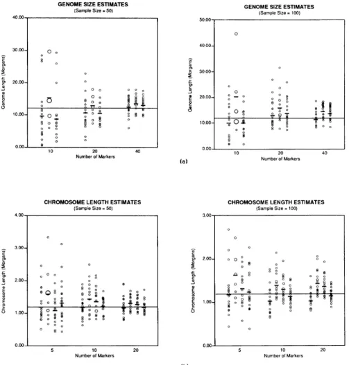
Genome length estimates: Genome length was estimated by methods 1, 2 and 3 for 10 chromosomes each of length 1.2 Morgans. All experiments were replicated 20 times for sample sizes of 50 and 100 meioses. T h e results are summarized in Figure la.

In general, estimates derived by all methods con- verged toward G (12 Morgans) as the number of marker loci studied increascd for a particular sample size. T h e average value of G over the 20 replications is presented below for 10, 20 and 40 markers, respectively. For method 1 and n = 50, the mean of the estimates was 10.20, 11.17, and 12.96 Morgans; for n = 100, the mean estimate was 10.82, 13.77 and

(4)

Chakravarti, Lasher and Reefer

GENOME SIZE ESTIMATES

(Sample Size = 50)

0 0

10

Number of Markers

20 40

CHROMOSOME LENGTH ESTIMATES

(Sample Size = 5 0 )

F

E O O

:

O

2.00

1 .00

I o

8 0

0.00

5 10 20

GENOME SIZE ESTIMATES

(Sample Size = 100)

50'001

0

40.00

0

10 20 40

CHROMOSOME LENGTH ESTIMATES

(Sample Size = 100)

0 0

0

5 10 20

FIGURE 1.-Estimation of genome length for (a) 10 chromosomes each of length 1.2 Morgans, and (b) 1 chromosome of length 1.2 Morgans, as a function of the sample size of meioses and number of markers studied. Each experiment was replicated 20 times. The G values are plotted with relative frequency indicated by the area of the circle. The average value is indicated by a - mark; the true value is marked by a line across the graph. The four series of values are those corresponding to methods 1, 2, 3 and 4, respectively.

(5)

worse as the sample size was increased. For method 3, no consistent effect of increasing sample size was observed.

Figure l a demonstrates two specific features of the estimation procedures. First, method 1 tends to underestimate G , but the bias becomes negligible as the number of markers (m) and/or the number of meioses ( n ) increases. However, method 2 overestimates G,

and this bias remains when n and m are increased. Method 3 has some properties of method 1, but also gives biased G values when n and m are increased. Second, there is considerable variability between the individual estimates of G among all methods, and qualitatively this variation decreases as n and m increase.

G was also estimated for a single chromosome of length 1.2 Morgans for samples of 50 and 100 meioses by methods 1, 2, 3 and 4. Again, experiments were replicated 20 times. These results are shown in Figure

l b . For all methods, the mean estimate is presented for 5 , 10 and 20 markers, respectively.

Method 1 provided a reasonable estimate of the single chromosome length in all cases. For 50 meioses, the estimate became more accurate as the number of markers increased, the mean being 1.24, 1.23 and

1.22 Morgans. For 100 meioses, the mean estimate dropped from 1.22 Morgans to 1.07 Morgans as the number of markers was increased from 5 to 10. T h e mean value was unchanged between 10 and 20 markers, but the standard deviation of the estimates de- creased.

Mean estimates derived by method 2 approached G

as the number of marker loci increased for 50 meioses. For 100 meioses, 10 markers provided a slightly better mean estimate than did either 5 or 20 markers. How- ever, Method 2 again consistently yielded an over- estimate. T h e mean was 1.65, 1.49 and 1.36 Morgans for n = 50 and was 1.67, 1.43 and 1.48 Morgans for n = 100.

Once again, method 3, provided less inflated estimates than method 2. Mean values were 1.13, 1.41 and 1.33 Morgans for n = 50. For n = 100 the mean value was 1.36, 1.34 and 1.40 Morgans.

For method 4, increasing the number of marker loci increased the accuracy of the estimates for both sample sizes. Additionally, increasing the sample size from 50 to 100 meioses generally increased the accuracy of the estimates. T h e mean estimate for n = 50 was 1.37, 1.26 and 1.23 Morgans. For n = 100, the mean estimate was 1.28, 1.18 and 1.19 Morgans.

When estimating the length of an individual chromosome, method 4 performs the best, as expected. However, of the other methods, the maximum likelihood estimator is the best, particularly when 50 meioses are studied. In general, methods 2 and 3

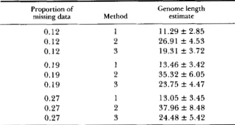
TABLE 1

Genome size estimates with missing data

Proportion of

missing data Method

Genome length estimate

0.12 1 11.29 f 2.85

0.12 2 26.91 f 4.53

0.12 3 19.31 f 3.72

0.19 1 13.46 f 3.42

0.19 2 35.32 f 6.05

0.19 3 23.75 f 4.47

0.27 1 13.05 f 3.45

0.27 2 37.96 f 8.48

0.27 3 24.48 f 5.42

Mean and standard deviation of the estimates of genome length for 10 chromosomes each of length 1.2 Morgans. Each experiment was replicated 20 times.

always give overestimates, whereas at TZ = 100, method

1 gives an underestimate.

Missing data: T h e original cross simulated for each of the missing data experiments was composed of 2n

= 100 marker loci and 2m = 40 meioses. We set the number of loci studied in common (2p) to be 10, 6 or 2 and subsequently computed the average number of meioses ( r i ) , the average number of marker loci (Gz),

and the proportion of missing data ( a ) for each. For

cy of 0.12, 0.19 and 0.27, ri was 38, 32 and 27, while Gz was 13, 12 and 11, respectively.

Genome length was estimated by methods 1, 2 and 3. T h e mean of the estimates from 20 independent replications of each experiment is shown in Table 1. As expected, the estimates generally become less accurate as the proportion of missing data was increased. Of the three methods used, only method 1 provided a reasonable estimate in all cases, with the mean ranging from 11.29 to 13.46 Morgans. Methods 2 and 3 provided gross overestimates in all cases, with the mean ranging from 26.91 to 37.96 Morgans for method 2 and from 19.31 to 24.48 Morgans for method 3.

Variation in chromosome lengths: One probable drawback of the maximum likelihood method and Equation 6 is the assumption of equal chromosome lengths. When chromosome lengths in a genome are variable, there are two possible effects on the estimation of G . First, the probability of synteny is larger than Ilk and this would alter the distribution of 0

assumed in the analysis. This is because the probability of synteny is cy =

2

L ? / G 2 = (1

+

&L2)/k where L and :a are the average and variance of chromosome lengths, and L, is the genetic length of the ith (i = 1,

(6)

-252430

?? -252440

3

r

$

-252450

-252460

-252470

0.4 0 6 0 8 0.88

I I I I I

1 0

1 2 1.4 1.6 1 8 Length (L)

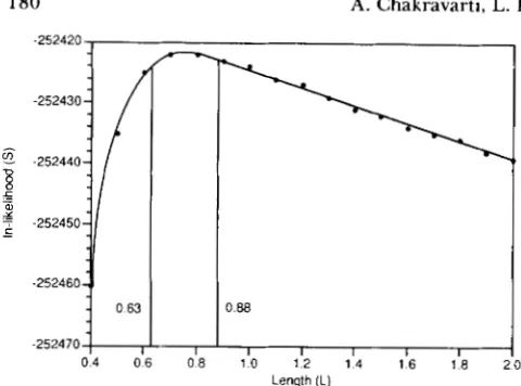
FIGURE 2.-A plot of In-likelihood of the Xzphophorus linkage data versus average genetic length per chromosome. The vertical lines delineate the 95% confidence limits.

increase the proportion of unlinked loci relative to the average. T h e exact magnitude of these effects cannot be theoretically predicted, and so we resorted to computer simulations.

We considered a genome with

k

= 10 chromosomes of lengths 30, 50, 70, 90, 110, 130, 150, 170, 190 and 2 10 cM. Such a genome has a total length of 12 Morgans and an average chromosome length of 1.2 Morgans, as before. We sampled 100 meioses and chose 20,40 and 80 markers. These expyiments were replicated 20 times and we computed G by assuming equal chromosome lengths for method 1. As a comparison, method 2, that does not depend on such assumptions, was also used on the same data. Our results show that for method 1, the estimated genome length was 13.87 f 4.34, 12.64 k 1.65, and 12.95 k

1.52 for m = 20, 40 or 80 markers. These estimates for method

2

were 16.22 2 6.03, 15.05 f 1.81 and 15.44 f 1.50, respectively. Comparisons of these values to the

6

values obtained when chromosomes of

equal length were simulated ( m = 20 and 40 markers only) show values of 13.77 f 4.90 ( m = 20) and 12.14

& 2.64 ( m = 40) under method 1, and 16.59 k 5.33 ( m = 20) and 15.20 k 2.67 ( m = 40) under method 2. Therefore, increasing the number of markers gives a more precise estimate of G, but method 2 consistently provides overestimates. In conclusion, the maximum likelihood method performs very well even with 40 markers, and even if equal chromosome lengths are assumed. It is interesting to observe that the G value was more dependent on the estimation method than on whether or not chromosomes were of equal length.

Xiphophorus linkage data: Because the integrity and accuracy of method 1 was maintained when data were missing and when chromosome lengths were unequal, this method was used to estimate genome length from partial linkage data of Xzphophorus (MOR-

IZOT et al. 1990). T h e Xzphophorus data consisted of 76 protein and enzyme coding loci segregating in 87

TABLE 2

The degree of genome coverage

mrioses markers Expected cover-

No. No.

(n) ( m ) age 2 s~ nm

50 10 0.382 k 0.044 500 20 0.6 15 f 0.056

40 0.846 f 0.049

100 10 0.490 f 0.064

k:gRl

1000

1

20 0.734 f 0.068 2000

40 0.923 f 0.044 4000

Given n and m , and assuming k = 10 and L = 1.2, the expected value and standard deviation of the proportion of genome covered was calculated from BISHOP et al. (1983).

crosses which produced 26 14 offspring. The number of polymorphic loci per cross varied from two to 4 1, but averaged more than 20 loci per cross. The details of the loci studied and the crosses are given in MORI- ZOT et al. (1991). By using the maximum likelihood me_thod the average genoye length per chromosome is L = 0.76

+-

0.09. Thus, G = 18.25 f 2.21 Morgans since

k

= 24. Figure 2 shows the plot of In-likelihood values versus L , from which these values are calcu- lated. This figure also gives the 95% confidence limits on L as (0.63, 0.88) Morgans; the 95% confidence limits on G being (15.12, 21.12) Morgans.

A second estimate of G was also obtained by method

2

(HULBERT et al. 1988). There were a total of 1921 pairwise locus tests; 61 of these comparisons with sample size 10 o r fewer meioses were ignored. Of the remaining 1860 tests, 68 comparisons gave lod scores 3 or greater. These data gave a genome length estimate of 31.88 Morgans, close to two times that obtained by the maximum likelihood method. This over- estimate is entirely consistent with the results of our computer simulations.

DISCUSSION

T h e previous results clearly demonstrate that genome length can be estimated by a variety of methods. When linkage data are complete the two basic methods, the maximum likelihood and the method-of-moments estimators, can perform equally well. However, when the data are not complete or when the chromosome lengths are variable, the maximum likelihood method is superior and should be the one used. It is instructive to consider the reliability of the estimate

of G in relation to the expected proportion of the genome covered or assayable by the linkage experiment. BISHOP et al. (1983) provide formulas for com- puting the expected proportion and the standard deviation of the genome covered (the total swept radius) given values of the number of individuals ( n ) , the number of markers ( m ) , the number of chromosomes

(7)

chromosome of length 1.2 Morgans, the proportion of the chromosome covered by the markers considered in our simulations is 0.946 or greater. T h e independence of individual linkage tests as implicit in both methods is thus violated, but the effect is less serious on the maximum likelihood method than on the method-of-moments. For a genome with

k

= 10 chromosomes, the expected proportion of coverage is shown in Table 2 . Comparison of these values with the

6

values in Figure 1 shows that the genome length estimate is not reliable unless m 2 20 when n = 5 0 or n = 100; that is when the coverage is 61.5% or greater. Note that when n = 50 and m = 20, 1000 genotypings are performed. When m = 10 and n = 100, an equal number of genotypings are performed, but the genome coverage is 49% vs. 61.5% and

6

is underesti- mated. This demonstrates that, for a fixed number of genotypings, it is useful to study more markers rather than more meioses to obtain an accurate estimate of genome length.

A crucial assumption in both the methods considered is the mutual independence between locus pairs. In the method of moments estimator, the swept radius from overlapping locus pairs are not independent and are “double counted.” This effect is more pronounced as marker locus density increases and is an explanation for the consistent overestimation of G . In the maximum likelihood method we also assume that each pairwise term is independent. This is also clearly false for overlapping loci but does not seem to have a pronounced effect. T h e reason appears to be that we consider all possible pairs, linked and unlinked, and that for any two randomly picked locus pairs the correlation is expected to be small. As shown in Ap- pendix 11, this average correlation is 2% or smaller. We believe this is the reason for the efficiency of the maximum likelihood method.

T h e maximum likelihood method, as implemented in this paper, is restricted to no interference and backcross data. However, Equation 6 is easily modified to include other types of linkage crosses, such as an intercross. Also, Equation 4 can be easily modified to include chiasma interference, such as with the Kosambi map function. T h e effects of interference are, however, more difficult to study since there are no models of chiasma interference that are readily applicable to computer simulation. T h e effect of interference can be studied empirically once a complete linkage map of a genome is available.

We thank Drs. D. Weeks, E. Lander and the reviewers for m n m e n t s 0 1 1 o u r manuscript. This study was supported by National

Institutes of Health (NIH) grants GM33771 and RCDA HD00774 t o A. C;. This research was also supported in part by a grant from t h e Pittsburgh Supercomputing Center through the NIH Division of Research Resources Cooperative agreement U41 RR04154.

LITERATURE CITED

BISHOP, D. T., C. CANNINGS, M. SKOLNICK and J. A. WILLIAMSON, 1983 The number of polymorphic DNA clones required to map the human genome, pp. 18 1-200 in Statistical Analysis of

DNA Sequence Data, edited by B. S . WEIR. Marcel Dekker, New York.

BOTSTEIN, D., R. L. WHITE, M. SKOLNICK and R. W. DAVIS, 1980 Construction of a genetic linkage map in man using

restriction fragment length polymorphisms. Am. J. Hum. Ge- net. 32: 314-331.

HALDANE, J. B. S., 1 9 1 9 T h e combination of linkage values, and the calculation of distance between the loci of linked factors. J. Genet. 8: 299-309.

HULBERT, S. H., T. W. ILOTT, E. J. LECG, S. E. LINCOLN, E. S.

LANDER and R. W. MICHELMORE, 1988 Genetic analysis of the fungus, Bremia lactucae, using restriction fragment length polymorphisms. Genetics 120 947-958.

IMSL MATH/LIBRARY USER’S MANUAL: FORTRAN Subroutines for Mathematical Applications, 1987 Version 1 .O, pp. 56 1-565, 569-572. IMSL, Inc., Houston.

LANDER, E. S . , P. GREEN, J. ABRAHAMSON, A. BARLOW, M. J. DALY, S . E. LINCOLN and L. NEWBURG, 1987 MAPMAKER: an

interactive computer package for constructing primary genetic linkage maps of experimental and natural populations. Ge-

nomics l: 174-1 8 l .

MORIZOT, D. C.. S. A. SLAUGENHAUPT, K. D. KALLMAN and A. CHAKRAVARTI, 1991 Genetic linkage map of fishes of the genus Xiphophorus (Teleostei: Poeciliidae). Genetics 127: 399- 410.

MORTON, N. E., 1955 Sequential tests for the detection of linkage. Am. J. Hum. Genet. 7: 277-318.

Communicating editor: B. S. WEIR

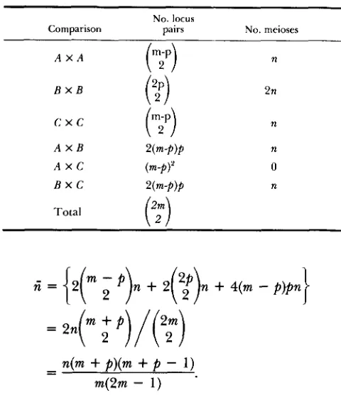
APPENDIX I

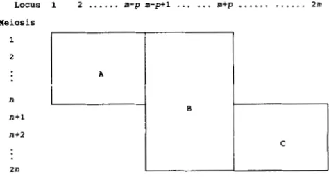
Characteristics of a mixed cross: Consider two crosses each with n meioses and m

+

p

loci but 2p loci studied in common as shown in Figure 3. Thus, there are three groups of markers A , B , C with sample sizes

n, 2n and n, respectively, and consisting of m

-

p , 2p,

and m

-

p

markers, respectively. T h e average number of markers studied

(m),

weighted by the sample size, is:

rit = ( 2 ( m - p)n

+

2 p . 2n1/4n

= (m

+

p ) / 2 .

We calculate the average number of meioses ( f i ) per locus pair by considering the various numbers of locus pairs and their sample sizes using Table 3. Thus,

LOCUS 1 2

...

m-p m - p + l

... ...

m+p

_...

... 2m Meiosis

2

n

n+l

n+2

2n

(8)

TABLE 3 TABLE 4

T h e numbers of locus pairs and meioses from two independent backcrosses with a fraction of common loci

Comparison

No. locus

pairs No. meioses

-

n(m + P)(m

+

P

-

1)

m(2m - 1 )

In comparison to a single equivalent cross the proportion of missing data is calculated as

f f = l - & & .

O n the other hand if a is fixed, then

p

may be calculated by inverting the above equation:

p

= { d l

+

4P2m(2m

-

1 )

-

(2m - 1)

I-

/ 2

=

~ J m ( 2 m

-

1 ) - m

when m is large and where

P

= 1

-

a. Thus, for fixed values of a, m and n , p may be calculated. This is helpful for simulating crosses with a predetermined proportion of missing data.

APPENDIX I1

Correlation between locus pairs: Consider the three ordered loci ABC studied in a backcross experiment with known linkage phase and interlocus recombination values of and 02, respectively. T h e expected frequencies of the four classes of progeny are provided in Table 4. Consider now the locus pairs A B

and AC which overlap in the A

-

B segment. Let R1 and R1+ 2 be random variables denoting the number

of recombinants between A and B, and, A and C, respectively. Then, R 1 = a

+

b and R1 + 2 = b

+

c, and,

Probabilities of recombinant classes from a 3-point backcross

Class Probability Observed No. Double recombinant & = B I O n a

Recombinant A-B

6

= 01(1-e2) b

Recombinant B-C ₅= ( 1 -&)O? C

Nonrecombinant ₅= (l-O,)(I-Od d

Total 1 n

E(R1) = n6'1

E(RI + z ) = no1 + 2

V(R1) = n6'1(1

-

0,)

V(RI + z ) = n6'1 + 2 ( 1

-

6'1 + 2 )

where 6'1 + 2 = O1

+

6'2

-

2d102 assuming no chiasma

interference; E and V are the expectation and variance, respectively. Then,

Cov(R1, R1+2) = COV(U, b )

+

COV(U, C)

+

COV(b, c)

+

V(b)

= n6'1(1

-

B2

-

+ 2 )

= n6'1(1 - el)( 1

-

2 6 ' 2 ) .

If ~ ( 6 ' 1 , 6'1 + 2) denotes the correlation between R 1 and

RI + 2 , then,

Note that if 6'2 = 0 then p = 1; if O2 = then p = 0, as

expected. Finally, if 6'1 = 82 = 8 then,

( 1

-

2 q 2 p2(6') = 2 [ 1

-

28(1

-

6')J'

T h e correlation p decreases as 8 increases, as expected, and takes the maximum value of l / & = 0.71 as 8 -+ 0.

Consider now a linkage experiment with m markers on k chromosomes, with m/k markers per chromosome on average. There are M = m(m - 1 ) / 2 pairwise locus comparisons overall, of which correlations can exist among only a subset of pairwise comparisons that arise from a chromosome. Since there are M terms in the In-likelihood in Equation 6 there are a total of M ( M

-

1 ) / 2 correlations, considering all locus pairs. Fur- thermore, with m/k loci per chromosome, there are P

= m(m/k - 1)/2k terms per chromosome in Equation

6 . Consequently, for all k chromosomes a maximum of KP(P - 1 ) / 2 correlations can exist. Thus, at high marker density (6' + 0), an upper bound to the maximum correlation is,

k P ( P - 1 ) / 2

Pmax

M ( M

-

1 )

.

When k = 10 and m = 40, M = 780 and P = 6 and