Shrinkage-Based Variable Selection Methods for Linear Regression and Mixed-Effects Models

(1)

sion and Mixed-Effects Models. (Under the direction of Professors H. D. Bondell and S. K. Ghosh).

In this dissertation we propose two new shrinkage-based variable selection ap-proaches. We first propose a Bayesian selection technique for linear regression mod-els, which allows for highly correlated predictors to enter or exit the model, simul-taneously. The second variable selection method proposed is for linear mixed-effects models, where we develop a new technique to jointly select the important fixed and random effects parameters. We briefly summarize each of these methods below.

The problem of selecting the correct subset of predictors within a linear model has received much attention in recent literature. Within the Bayesian framework, a popular choice of prior has been Zellner’s g-prior which is based on the inverse of empirical covariance matrix of the predictors. We propose an extension of Zellner’sg -prior which allow for a power parameter on the empirical covariance of the predictors. The power parameter helps control the degree to which correlated predictors are smoothed towards or away from one another. In addition, the empirical covariance of the predictors is used to obtain suitable priors over model space. In this manner, the power parameter also helps to determine whether models containing highly collinear predictors are preferred or avoided. The proposed power parameter can be chosen via an empirical Bayes method which leads to a data adaptive choice of prior. Simulation studies and a real data example are presented to show how the power parameter is well determined from the degree of cross-correlation within predictors. The proposed modification compares favorably to the standard use of Zellner’s prior and an intrinsic prior in these examples.

(2)

(3)

by Arun Krishna

A dissertation submitted to the Graduate Faculty of North Carolina State University

in partial fullfillment of the requirements for the Degree of

Doctor of Philosophy

Statistics

Raleigh, North Carolina 2009

APPROVED BY:

Dr. Hao H. Zhang Dr. Lexin Li

Dr. Howard D. Bondell Dr. Sujit K. Ghosh

(4)

DEDICATION

(5)

BIOGRAPHY

Arun Krishna was born on July 1st_{, 1980 in Bangalore, India. He graduated from} high school in 1997 and joint Manipal Institute of Technology, Manipal, India, to pursue a degree in Electrical Engineering, he obtained his bachelors degree in 2001. He then decided to fulfill his dream and come to America.

(6)

ACKNOWLEDGMENTS

First and foremost I would like to thank my advisors Dr. Howard Bondell and Dr. Sujit Ghosh, without whose direction and guidance this dissertation would not exists. I would also like to thank my committee members Dr. Helen Zhang and Dr. Lexin Li whose helpful suggestions and comments helped to strengthen this dissertation.

I would like to thank the Department of Statistics, North Carolina State Univer-sity for their support. My advisors and I would like to thank the executive editor and the three anonymous referees for their useful comments to our paper, “Bayesian Variable Selection using Adaptive Powered Correlation Prior”. We would also like to thank Steven Howard at United States Environmental Protection Agency (EPA) for processing and formatting the CASTNet data for our application.

(7)

LIST OF TABLES

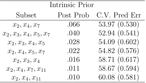
Table 1.1 Penalized Regression methods and their corresponding penalty terms . 24

Table 2.1 For Case 1, Comparing Average Posterior Probabilities, corresponding to the case 1: p= 4, averaged across 1,000 simulations. % Selected is the number of times (in %) each model was selected as the highest posterior model out of 1000 replications. Zellners represents use of Zellners prior as in (2.19). PoCor represents our proposed modification as in (2.14). Intrinsic Prior represents the fully automatic procedure proposed by Casella and Moreno (2006) . . . 43 Table 2.2 Case 2, Comparing Average Posterior Probabilities, corresponding to

the case 2: p= 12, averaged over 1,000 Simulations. % Selected is the number of times (in %) each model was selected as the highest posterior model out of 1000 replications. Zellners represents use of Zellners prior as in (2.19). PoCor represents our proposed modification as in (2.14). Intrinsic Prior represents the fully automatic procedure proposed by Casella and Moreno (2006) . . . 44 Table 2.3 Comparing Posterior Probabilities and average prediction errors for the

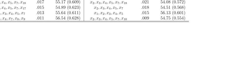
models of the NCAA Data. The entries in parenthesis are the standard errors obtained by 1000 replications. . . 45 Table 2.4 Posterior Probabilities and average prediction errors for the models of

the NCAA Data using the Intrinsic Priors. The entries in parenthesis are the standard errors obtained by 1000 replications. . . 46

Table 3.1 Comparing the median KullbackLeibler discrepancy (KLD) from the true model, along with the percentage of the times the true model was se-lected (%Correct) for each method, across 200 datasets. R.E represents the relative efficiency compared to the oracle model. %CF, %RF corresponds to the percentage of times the correct fixed and random effects were selected , respectively. . . 73 Table 3.2 Variables selected for the fixed and the random components for the

(10)

(11)

LIST OF FIGURES

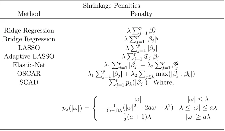
Figure 2.1 Plot of λ vs. Log[m(y_|X, π, λ)], maximized over π _∈ (0,1), corre-sponding to case 1: p= 4. Averaged over 1,000 simulations. The vertical line represents the location of the global maximum.. . . 40 Figure 2.2 Plot of λ vs. Log [m(y_|X, π, λ)], maximized over π _∈ (0,1),

corre-sponding to case 2: p= 12, averaged over 1,000 simulations. The vertical line represents the location of the global maximum.. . . 41 Figure 2.3 Plot of λ vs. Log[m(y_|X, π, λ)], maximized over π _∈ (0,1),

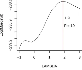
corre-sponding to the NCAA Dataset. The vertical line represents the location of the global maximum. . . 42

Figure 3.1 The location of the 15 Sites that were used for our analysis. The _∇ represents the 4 sites used for the overlay plots in Figure 3.4.. . . 69 Figure 3.2 Site (individual) profile plot to assess the seasonal trend in Nitrate

concentration over each 12 month period, for the CASTnet dataset. . . 70 Figure 3.3 Box Plot to assess heterogeneity among the 15 sites in the measured

Nitrate concentration corresponding to the CASTnet dataset. . . 71 Figure 3.4 Plot of the observed LOG(TNO)₃ concentration represented by the

(12)

Chapter 1 Introduction

In the statistical literature, the problem of selecting variables/predictors has re-ceived considerable attention over the years. Variable selection has two main goals, easy model interpretation (sparse representation) and prediction accuracy. In prac-tice, statistical data often consist of a large number of potential predictors or explana-tory variables, denoted by x1,x2, . . . ,xp. Usually not all these variables contribute to the explanation of a particular quantity of interest, the response variable y. The variable selection problem arises when it is of particular interest to identify the subset p′ _≤_p_{of relevant predictor variables. This then results in removing the} noninforma-tive variables in order to improve the predictability of the models and parsimoniously describe the relationship between the outcome and the predictive variables.

(13)

1.1 Variable Selection in Linear Regression

Mod-els

Most statistical problems involve determining the relationship between the re-sponse variable and the set of predictors. This can often be represented in a linear regression framework as

y=Xβ+ǫ, (1.1)

where y is an n_×1 vector of responses and X = (x′₁,_{· · ·},x′_p)′ _{is an} _n_×_p _matrix of known explanatory variables, with β = (β1, . . . , βp)′ a p×1 vector of unknown

regression parameters, and ǫ _∼ N(0, σ2_I_{), where} _N₍₀_{, σ}2_I_{) denotes a multivariate}

normal distribution with mean vector zero and variance-covariance matrix σ2_I_{. We}

assume throughout that theX’s andy’s have been centered so that the intercept may be omitted from the model. Under the above regression model, it is assumed that only an unknown subset of the coefficients is nonzero, so that the variable selection problem is to identify this unknown subset.

In the context of variable selection we begin by indexing each candidate model with one binary vector δ = (δ1,· · · , δp)′, where each element δj takes the value 1 or 0 depending on whether a predictor is included or excluded from the model. Given δ _{∈ {}0,1_}p_{, the linear regression model assumes}

y_|δ,_βδ, σ2 _∼N(_Xδβδ, σ2I), (1.2)

where_Xδ and_βδ are the design matrix and the regression parameters corresponding to the non-zero elements of δ, respectively, and σ2 _{is the unknown error variance for}

model δ. Notice that_Xδ is a matrix of dimension n_×p_δ where p_δ =Pp

j=1δj and

(14)

1.1.1 Subset Selection

Subset selection methods (Miller, 2002) such as all subsets, forward selection, backward elimination and STEPWISE have been widely used by statisticians to select significant variables. The all subsets selection method performs an exhaustive search over all possible subsets in model space. For instance, given the linear model in (1.1) the total number of possible sub-models is 2p_{. After enumerating all possible models} in consideration, the all subset method then selects the best model using a given criterion. The main drawback of this method is that it is computationally intensive and could be time consuming, especially if the number of predictors (p) is large.

To obtain the ‘best’ model using subset selection, Mallows (1973) proposed a Cp statistic (we denote it byC_δ) which involves estimating the out-of-sample prediction error for each model indexed by δ. We use this statistic as a criterion to compare different subsets of regression models. The criterion is computed as

C_δ = ||y−Xδβδˆ ||

2

ˆ

σ2 −n+ 2pδ, (1.3)

where ˆσ2 _{is the unbiased estimate of the error variance based on the full model. The}

model with the minimum value of C_δ is then termed the ‘best’ model.

Information-based criterion approaches attempt to find the model with the small-est Kullback-Leibler (Kullback and Leibler,1951) divergence from the true but un-known data generating process. Akaike Information Criterion (Akaike, 1973) is one such estimate of this distance. Ignoring the constant terms the AIC for modelδ in a linear regression framework can be computed as

AIC_δ =nlog_||y₋Xβˆ_||2+ 2p_δ (1.4)

(15)

penalty on the degrees of freedom. The BIC criterion is given as

BIC_δ =nlog_||y₋Xβˆ_||2+ log(n)_×p_δ, (1.5)

wheren is the total number of observations. Again, the model which minimizes (1.5) is selected. The BIC is consistent for model selection. I.e., if the true model p0 is in

the class of all models considered, the value of p_δ that minimizes (1.5) converges to the true model (p0) asn → ∞.

To avoid the burden of enumerating all possible (2p_{) models, methods such as} forward selection or backward elimination are used to find the best subset, either by adding or deleting one variable at a time or by a combination of the two, such as in STEPWISE. In each step the best predictor is included or excluded according to some criterion, e.g., the F-statistic, AIC or BIC. However, these methods are extremely unstable and are very sensitive to small changes due to their inherent discreteness (Breiman, 1996).

1.1.2 Penalized Least Squares

Though subset selection is practical and widely used as a method to find the best model, it has many drawbacks. Breiman (1996) discusses the lack of stability of the subset selection procedures, where a small change in the data could result in a large change in their predictive error and can result in very different models being selected. In practice, these methods could be very time consuming due to being computationally intensive, especially when the number of predictors is large.

To overcome these obstacles, the use of penalized regression, or regression shrink-age, has emerged as a highly successful method to tackle this problem. The idea behind penalized least squares is to obtain the estimates for the regression coeffi-cients by minimizing the penalized sum of squared residual

||y₋Xβ_||2+ p X

j=1

(16)

where Pp

j=1pλ(|βj|) is the penalty term corresponding to the regression coefficients,

andλ is a non-negative tuning parameter. Several forms of the penalty function have been proposed. These are summarized in Table 1.1.

The penalized least square technique first proposed by Hoerl and Kennard (1970), called Ridge regression, minimizes the residual sum of squares by imposing a bound on the l2 norm of the regression coefficients. By introducing this penalty they succeeded

in shrinking the least square estimates continuously toward zero and achieving a better predictive performance than the Ordinary Least Squares (OLS). Due to the continuous shrinking process it results in being more stable and not sensitive to small changes in the data as in subset selection. Though this method does not perform variable selection as it does not set the coefficients to zero, it is sometimes used in combination with other penalty terms which do perform variable selection.

Adopting the good quality (continuous shrinkage) of the ridge regression (Ho-erl and Kennard, 1970) penalty and combining it with the good features of subset selection, Tibshirani (1996) proposed the Least Absolute Shrinkage and Selection Op-erator (LASSO). This method introduces anl1 penalty (Pp_j₌₁|βj|) on the regression

coefficients. Due to the geometric nature of the l1 penalty the LASSO does both

continuous shrinkage as well as variable selection by having the ablity the regression coefficients to zero. The LASSO estimates for the regression parameters are defined as

ˆ

β= arg min β ||

y₋Xβ_||2+λ p X

j=1

|βj_|, (1.7)

whereλis a non-negative tuning/regularization parameter. Asλincreases, the coeffi-cients are continuously shrunk towards zero, and some coefficoeffi-cients are exactly shrunk to zero for a sufficiently large λ. A plethora of penalized regression techniques have been proposed by modifying the LASSO penalty to accommodate other desirable properties. We shall discuss a few.

(17)

computationally efficient.

In the presence of highly correlated predictors it has been show empirically that the performance of the LASSO is sub-par compared to the ridge regression in pre-dictive performance (Tibshirani, 1996). With this in mind, Zou and Hastie (2005) proposed the ‘Elastic-Net’ procedure, whose penalty term is a convex combination of the LASSO penalty (Tibshirani, 1996) and the ridge regression (Hoerl and Kennard, 1970) penalty, as shown in Table (1.1). The ‘Elastic-Net’ simultaneously performs au-tomatic variable selection with the help of thel1penalty while encouraging a grouping

effect by selecting groups of highly correlated predictors, rather than simply elimi-nating some of them from the model arbitrarily.

Along the same lines as the ‘Elastic-net’, Bondell and Reich (2008) proposed a clustering algorithm called the Octagonal Shrinkage and Clustering Algorithm for Regression (OSCAR) which uses a convex combination of the LASSO penalty and a pairwise L_∞ penalty (Table 1.1). This method not only shrinks the unimportant coefficients to zero with the help of the LASSO penalty; it also encourages highly correlated predictors that have a similar effect on the response to form predictive clusters by setting them equal to one another. Hence, the OSCAR eliminates the unimportant predictors while performing supervised clustering on the important ones. To overcome the drawback that the LASSO shrinkage method produces biased estimates for the large coefficients, Fan and Li (2001) proposed a variable selection approach via non-concave penalized likelihood where a Smoothly Clipped Absolute Deviation (SCAD) penalty is used (see Table 1.1). They proposed a general theoret-ical setting to understand the asymptotic behavior of these penalized methods called the “Oracle property”. The formal definition in the context of a linear regression framework is as follows.

Definition 1. Let the true value of β be given by

β₀ = (β10, β20, . . . , βpo)′ = (β′10,β′20)′, (1.8)

(18)

de-note the penalized regression estimates obtained. The penalized likelihood estimator βˆ

enjoys the ‘Oracle’ property if the following hold true.

(i) The true zero coefficients are estimated as zero with probability tending to 1, that is, limn→∞P( ˆβ2 = 0) = 1.

(ii) The penalized regression estimates of the true non-zero coefficients are √n con-sistent and asymptotically normal; that is, √n( ˆβ₁ ₋ β₁₀) _→d N(0, I−1(β10)),

where I(β₁₀) is the Fisher information matrix, knowing thatβ₂ =0.

Hence an estimator that satisfies these conditions performs as well as if the true model were known beforehand. Zou (2006) proposed another penalized method called the adaptive LASSO in which adaptive weights are used to penalize the different regression coefficients in thel1 penalty. That is, large amount of shrinkage are applied

to the zero-coefficients while smaller amounts are used for the non-zero coefficients. This then results in an estimator with improved efficiency, as opposed to the LASSO which gives the same amount of shrinkage to all the coefficients. The adaptive LASSO estimates are defined as

ˆ

β = arg min β ||

y₋Xβ_||2+λ p X

j=1

¯

wj_|βj_|, (1.9)

where ¯wj are the adaptive weights, typically ~_wj _{= 1}_/_|_βj¯_|_{, with ¯}_βj _{the ordinary least}

squares estimate. The adaptive LASSO can now be thought of as a convex optimiza-tion problem with an l1 constraint. Zou demonstrated that the adaptive LASSO

es-timates can be obtained by using the highly efficient LARS algorithm (Efron, Hastie, Johnstone and Tibshirani, 2004) by making a small change to the design matrix. Zou further showed that the adaptive LASSO estimates enjoys the ‘Oracle’ property (Definition 1).

1.1.3 Bayesian Variable Selection

(19)

models. Given the conditional distribution ofy(1.2), the approach then proceeds by assigning a prior probability to all possible models indexed by δ along with a prior probability distribution to the model parameters (_βδ, σ2_{) in a hierarchical fashion}

P(_βδ, σ2,δ) =P(_βδ_|σ2,δ)P(σ2_|δ)P(δ). (1.10)

Posterior model probabilities are then used to select the ‘best’ model. With this set-up in mind, many variable selection techniques have been proposed by using different and innovative priors for the model parameters and the prior over model space. We shall discuss a few of these methods.

Mitchell and Beauchamp (1988) introduced the ‘spike and slab’ prior for β’s. They assume that the β’s are independent of σ and that the βj are also mutually independent. More explicitly, the prior for each βj is

P(βj_|δj) = (1₋δj)1_{0}(βj) +δj 1

2a1[−a,a](βj).

The prior for the inclusion indicators δ is given an independent Bernoulli distribu-tion with parameter wj. The hyperparameters are obtained using a Bayesian cross-validation and ‘best’ model is obtained using posterior probabilities.

George and McCulloch (1993, 1997) propose a mixture normal prior for the re-gression coefficients and an inverse-gamma conjugate prior on σ2_{. The difference}

between this method and the ’spike and slab’ prior is that they do not implicitly put a probability mass for βj = 0. Instead, forδj = 0, the corresponding prior on βj has a variance close to its mean (zero). As for the prior over model space, George and McCulloch suggests

p(δ)_∝πpδ₍₁₋_π₎p−pδ_, _(1.11) where p_δ =Pp

(20)

space

P(δ) =

1 2

p

. (1.12)

However, the drawback of using this prior is that it puts most of its mass on models of size p/2. For large p it is nearly impossible to enumerate all 2p _possible models. With this in mind George and McCulloch (1993,1997) introduce the SVSS (Stochastic Search Variable Selection) algorithm to search though model space by utilizing Gibbs sampling to indirectly sample from the posterior distribution on a set of possible subset choices. Models with high posterior probabilities can then be identified as the ones which most frequently appeared in the Gibbs sample.

More recently, Yuan and Lin (2005) showed that under certain conditions that the model with the highest posterior probability selected using their method will also be the model selected by LASSO. To show this, they proposed a double exponential prior distribution on the regression coefficients. As for the prior over model space they proposed

P(δ)_∝πpδ₍₁₋_π₎p−pδ_|_X′

δXδ|1/2, (1.13)

In a linear regression framework, Zellner (1986) suggested a particular form of a conjugate Normal-Gamma family called the g-prior, which can be expressed as

β_|σ2, g _∼ N(0,σ

2

g (X

′_X₎−1₎

σ2 _∼ IG(a0, b0), (1.14)

where g > 0 is a known scaling factor and a0 > 0, b0 > 0 are known parameters of

the Inverse Gamma distribution with mean a0

b0−1. The prior covariance matrix ofβ is the scalar multipleσ2_/g _{of the inverse Fisher information matrix, which concurrently}

(21)

selection the ‘g-priors’ are conditioned on δ to give

βδ|δ, g, σ2 _∼N(0,σ

2

g (X ′

δXδ)−1).

This particular prior has been widely adopted in the context of Bayesian variable selection due to its closed form calculations of all marginal likelihoods which is suitable for rapid computations over a large number of submodels. Its simple interpretation can be derived from the idea of a likelihood for a pseudo-data set with the same design matrix X as the observed sample.

George and Foster (2003) used the above ‘g-prior’ to establish a connection be-tween models selected using posterior probabilities and model selection criteria such as the AIC (Akaike, 1973), BIC (Schwartz, 1978) and the RIC (Foster and George, 1994). They showed that the ordering induced using the posterior probabilities is the same as the ordering obtained using any of the model selection criteria. They pro-posed an empirical Bayes method by maximizing the marginal likelihood of the data to obtain the estimates for the hyperparameters g and π. Similar results were also established by Fernandez et. al (2001) by using P(σ2₎ _∝ ₁_/σ2_{. This representation}

avoids the need for choosing a0, b0. To avoid the need to specify hyperparameters,

Casella and Moreno (2006) proposed a fully automatic Bayesian variable selection procedure where posterior probabilities are computed using intrinsic priors (Berger and Pericchi, 1996). Final model comparisons are made based on Bayes factors.

But the main drawback of all these methods is that they are not designed to handle correlated predictors. As including groups of highly correlated predictors together in the model can improve predictor accuracy as well as model interpretation (Zou and Hastie, 2005; Bondell and Reich, 2008). In Chapter 2 we propose a modification of Zellner’s g-prior (1.14) by replacing (X′_δXδ)−1 _{with (}_X′

δXδ)λ where the power λ _∈ R_{, controls the amount of smoothing of the regression coefficients of collinear}

(22)

proposed method encourages groups of correlated predictors to enter or exit the model simultaneously.

1.2 Introduction to Linear Mixed-Effects Models

Linear mixed-effects (LME) models are a class of statistical models which are used directly in many fields of application. LME models are used to describe the relationship between the response and a set of covariates that are grouped according to one or more classification factors. Mixed models have been commonly used to analyze clustered or repeated measures data. In this section we shall provide the reader with a general overview on the theory behind mixed models. We will also briefly describe the techniques commonly used to obtain the estimates for the fixed effects parameters and the variance components.

Consider a study consisting of m subjects, with response from each subject i = 1,2_{· · ·}, m measured ni times, and let N =Pm

i=1ni be the total number of

observa-tions. Let y_i be a ni_×1 vector of the response variable for subject i. Let Xi be the ni×p design matrix of explanatory variables, and β= (β1,· · ·, βp)′ be the vector of unknown regression parameters which are assumed to be fixed. Letbi = (bi1,· · · , biq)′

be a q_×1 vector of unknown subject-specific random effects, and Zi is the ni ×q known design matrix corresponding to the random effects. A general class of LME models can be written as

y_i =Xiβ+Zibi+ǫi. (1.15)

The random effectsbi andǫi are independent of each other and generally assumed to come from a normal distribution as shown

" bi ǫi

# ∼N

"

0

# , σ2

"

Ψ 0

0 Ini #!

. (1.16)

(23)

also be written as

y=Xβ+Zb+ǫ, b _∼N(0, σ2Ψ˜), ǫ_∼N(0, σ2I), (1.17)

where X = [X′₁, . . . ,X′_m]′ denotes a N _×p stacked matrix of Xi, and Z and ˜Ψ

denote block diagonal matrices which are given by

˜ Ψ=       

Ψ 0 . . . 0 0 Ψ . . . 0 ... ... ... ... 0 0 . . . Ψ

      

,Z =       

Z1 0 . . . 0

0 Z2 . . . 0

... ... ... ... 0 0 . . . Zm

       . (1.18)

Given (1.17) and b= (b1, . . . ,bm)′, the hierarchical formulation is written as

y_|b _∼ N(Xβ+Zb, σ2I),

b _∼ N(0, σ2Ψ˜). (1.19)

Integrating out the random effects, it can be shown that the marginal distribution of y follows

y _∼ N(Xβ,V˜)

where, ˜V = σ2₍_Z_Ψ_˜_Z′₊_I₎_, _(1.20)

(24)

1.2.1 The Maximum Likelihood and Restricted Maximum

Likelihood Estimation

Let us denote θ = (β′, V ech′₍_Ψ₎_{, σ}2₎′ _{to be a} _s_×_{1 combined vector of unknown} parameters, where V ech(Ψ) represents the q(q+ 1)/2 free parameters of Ψ. Hence the total dimension of θ is 1 +p+q(q+ 1)/2. Let Θ denote the parameter space for θ such that

Θ =_{θ :β_∈Rp_{, σ}2 _>₀_,_Ψ _{is non-negative definite}_}_. _(1.21)

Dropping out the constant terms, the log-likelihood function based on the LME model (1.17) is given by

LM L(θ) =−

1 2

N _×log(σ2) + log_|I +ZΨ˜_Z′_|₊ 1

σ2(y−Xβ)′(I+ZΨ˜Z′)−

1₍_y₋_Xβ₎

,

(1.22)

where ˜Ψ= Diag(Ψ, . . . ,Ψ) is a block diagonal matrix of Ψ’s. The maximum likeli-hood estimate (MLE) maximizes (1.22) over the parameter space Θ given in (1.21). Note that in certain situations the ML estimates may fall outside the boundary of the parameter space Θ, one could avoid this one would need to deal with constrained maximization, we shall discuss in detail at the end of section 1.2.2. For a known Ψ, the estimate forβ is given by

ˆ

β= (X′(I +ZΨ˜Z′)−1_X₎−1_X′₍_I₊_Z_Ψ_˜_Z′₎−1_y, _(1.23)

where the variance of ˆβ is given by X′V˜−1X. For Ψ= 0, notice that the estimate forβreduces to the OLS (ordinary least square) estimate. Again, for a knownΨand replacing β with ˆβ given in (1.23), and taking the derivative of (1.22) with respect toσ2 _{we see that the log-likelihood function is maximized at}

ˆ σ2 = 1

N n

(25)

WhenΨis unknown we obtain an estimate of it by maximizing (1.22) after replacing β and σ2 _{by (1.23) and (1.24), respectively.}

Maximum Likelihood estimators are functions of sufficient statistics and are √n consistent and asymptotically normal (see Searle, Casella and McCulloch, 1992). But the estimates of the variance components are biased downwards. The bias arises be-cause the method does not take into consideration the degrees of freedom lost due to the estimation of the fixed effects. To overcome this, Patterson and Thompson (1971) proposed the restricted maximum likelihood (REML) method to obtain unbiased es-timates of the variance components in an LME framework. The REML log-likelihood for the LME model in (1.15) is

LR(θ) = ₋1 2

(N ₋p)log(σ2) + log_|I +ZΨ˜Z′_|+ log_|X′(I +ZΨ˜Z′)−1X_|

+ 1

σ2

n

(y₋Xβ)′(I+ZΨ˜Z′)−1(y₋Xβ)o

. (1.25)

For a known Ψ, taking the derivative with respect to σ2 _{results in maximizing the}

function (1.25) at

ˆ

σ_R2 = 1 N ₋p

n

(y₋Xβˆ)′(I +ZΨ˜Z′)−1(y₋Xβˆ)o, (1.26)

where ˆβ is as given in (1.23), and p is the number of fixed effects. We see that the degrees of freedom for REML estimates for σ2 _{have been adjusted by the number of}

fixed effects.

1.2.2 Numerical Algorithms

(26)

(1987), Newton-Raphson (Lindstrom and Bates, 1988) and Fishers scoring algorithm (see McLachlan and Krishnan (1994) and Demidenko (2004) for a comprehensive review of each of these methods). In this section we shall discuss the EM algorithm in detail.

The EM Algorithm

Dempster, Laird and Rubin (1977) proposed a general class of algorithm to com-pute the maximum likelihood estimates of parameters in the presence of missing data. Laird and Ware (1982) and Laird, Lange and Stram (1987) adopted this formulation to LME model by treating the random effects as unobserved (missing) data. Hence, in the general EM setting we shall call the observed data y as incomplete data, and (y,b) as the complete data.

The EM algorithm has two main steps: the E-step where we compute the condi-tional expectation of the complete data log-likelihood assuming that the latent vari-ables (i.e. random effects) are unobserved; and the M-step, where we maximize the expected complete-data log-likelihood with respect to the parameters in the model, using numerical optimization techniques. This process is then repeated iteratively to obtain the final converged estimates.

Given the hierarchical setup in (1.19) and dropping out the constant terms, the complete-data log-likelihood is given as

L(θ_|y,b) =₋1 2

(

(N +mq)log(σ2) + log_|I+ZΨ˜_Z′_|₊||y−Xβ−Zb||

2₊_b′_{( ˜}Ψ₎−1_b

σ2

)

.

(1.27)

Given (1.27), the conditional distribution of b given θ and y is b_|y,θ _∼ N(ˆb,G), where the mean and the conditional variance are given by

ˆ

b = (Ψ)−1+Z′Z−1

Z′(y₋Xβ)

G = σ2(Z′Z+ (Ψ)−1)−1. (1.28)

(27)

θat theωth_{iteration. Given}_θ(ω)_{, we compute the conditional expectation}_E

b|y,θ(ω)

of the complete-data log-likelihood as

g(θ_|θ(ω)) = Z

L(θ_|y,b)f(b_|y,θ(ω))db, for all θ

= EnL(θ_|y,b)_|y,θ(ω)o, (1.29)

where L(θ_|y,b) is as given in (1.27). This defines the E-step. For the M-step, the updates estimate forθ is obtained by maximizing the objective function g(θ_|θ(ω)) to obtain θ(ω+1) such that

g(θ(ω+1)_|θ(ω))_≥g(θ_|θ(ω)). (1.30)

The process is now repeated iteratively until convergence to obtain the final estimates. The main drawback of the EM algorithm is its slow convergence, when the variance-covariance matrix Ψ is in the neighborhood of zero or in certain cases if ML/REML estimates ofΨare on the boundary of the parameter space. Many different extensions and modifications have been proposed to overcome the slow rate of convergence. For examples see Meng and Rubin (1993); Baker (1992); Liu and Rubin (1994); McLachlan and Krishnan (1997); Meng (1997); Lu, Rubin and Wu (1998); Meng and Van Dyk (1998).

(28)

as it involves unconstrained parameters for numerical optimization. See Lindstrom and Bates (1988); Pinhero and Bates (1996); Bates and DebRoy (2003).

1.3 Variable Selection in LME models

Variable selection for LME models is a challenging problem which has its appli-cation in many disciplines. As a motivational example, let us consider a recent study (Lee and Ghosh, 2008) of the association between total nitrate concentration in the atmosphere and a set of measured predictors using the U.S. EPA CASTnet data. The dataset consists of multiple sites with repeated measurements of nitrate concentration along with a set of potential covariates on each site. To analyze this data one could use an LME model, which takes into account the possible heterogeneity among the different study sites by introducing one or more site-specific random intercept and slopes, this model specification allows us the flexibility to model both the means as well as the covariance structure. But one would need to take care to fit the appropri-ate covariance structure of the random effects, as underfitting it might result in the underestimation of the standard errors for the fixed effects. Overfitting the covari-ance structure on the other hand, could result in near singularities (Lange and Laird, 1989). Therefore, an important problem in LME models is how to simultaneously select the important fixed and random effect components, as changing one of the two types of effects greatly affects the other.

(29)

1.3.1 Subset Selection

Information-based criteria are the most commonly used method to identify the important fixed as well as the important random effects in the model. This is done by computing the AIC (Akaiki, 1973) and BIC (Schwartz, 1978) for all plausible models in consideration. Let M_{represent the set of candidate models. Let}_M _denote

a candidate model such that, M _∈ M_{. Let} _θ_M _{= (}_β′

M, vech′(ΨM), σM2 )′ denote the vector of parameters under modelM. Given M, The AIC and BIC is computed as

AICM = −2LM L(ˆθM) + 2×dim(θM),

BICM = −2LM L(ˆθM) + log(N)×dim(θM), (1.31)

where ˆθM is the maximizer ofLM L(θ) given in (1.22) under modelM, and dim(θM) is the dimension ofθM. Given the LME model (1.15), the total number of possible sub-models includes all possible combinations resulting from the mean and the covariance structures, that is 2p+q_{. Hence, this method could result in being extremely time} consuming as well as computationally demanding especially ifp andq are very large. In order to slightly reduce the computation time Wolfinger (1993) and Diggle, Liang and Zeger, (1994) proposed the Restricted Information Criterion (which we denote by REML.IC). Using the most complex mean structure i.e. including all pos-sible fixed effects in the model, selection is first performed on the variance-covariance structure of the random effects by computing the AIC/BIC value for every possible covariance structure using the restricted log-likelihood given in (1.25). The degrees of freedom corresponds to the number of free variance-covariance parameters in Mq. Given the ‘best’ covariance structure, selection is then performed on the fixed effects. Hence, the number of possible sub-models evaluated for this procedure is the sum of the mean structures and the covariance structures in consideration. That is, given the LME model (1.15) the total possible models to enumerate is 2p_{+ 2}q_.

(30)

including all the random effects in the model, using the BIC. Once the fixed effects are chosen selection is then performed on the random effects. They further showed that this procedure is consistent and asymptotically efficient. But as seen from their simulation study,this method performs poorly when it is used to select the random effects.

To avoid enumerating a large number of possible sub-models, Morell, Pearson and Brant (1997) proposed a backward selection criteria to identify the important fixed and random effects. Given the full model, elimination is first performed on the fixed effect which do not have matching random effects. Once all the highest-order fixed effects are statistically significant, backward elimination of the fixed and the random effects is performed starting with the highest-order factors. At each step of the elimination of the fixed effect, the corresponding random effect can be considered for elimination. Though this method is much faster than enumerating all possible models it faces the drawback of being extremely unstable due to its inherent discreteness (Breiman, 1996).

Recently, Jiang, Rao, Gu, Nguyen (2006) proposed a ‘fence’ method in a more general mixed models setting, a special case being the LME model. The idea is to isolate a sub group of models called the ‘correct’ model by using a ‘statistical fence’ which eliminates the ‘incorrect’ models. The optimal model is then selected form this group within the fence according to some criteria., the statistical fence is constructed in the following way,

−LM L(ˆθM)≤ −LM L(ˆθ_M˜) +cn×ˆσ₍_M,_M˜₎, (1.32)

where ˜M _∈ M _{represents the full model, and (ˆ}_θM_,ˆ_θ_˜

M) are the local maximizers of LM L(ˆθM) andLM L(ˆθ_M˜) respectively, and where ˆσ₍_M,_M˜_{) =}

p

(31)

space, it could still result in being computationally intensive especially if the number of predictors (p, q) is large.

1.3.2 Bayesian Variable Selection for LME Models

A common approach to Bayesian variable selection in LME models is as follows. Again, let M_{denote the model space and let} _M _{denote a candidate model such that,}

M _∈M_{. Given} _M_{, we have}

y_|M,β_M, σ_M2 ,ΨM ∼N(XMβM,VM˜ ), (1.33)

where ˜VM is a block diagonal matrix of Vi,M = σ2M(Ini +Zi,MΨMZ

′

i,M) for i = 1, . . . , m, under modelM.

Given (1.33), the Bayesian selection approach is to assign a prior distribution to the model parameters (β,Ψ, σ2_{) for each model indexed by} _M _{in a hierarchical}

fashion. Such that

P(β_M,ΨM, σ2, M) =P(βM|M,ΨM, σ2)P(ΨM|M)P(σ2|M)P(M). (1.34)

Bayes theorem is then used to calculated posterior probabilities.

Using this hierarchical formulation, Weiss, Wang and Ibrahim (1997) proposed a Bayesian method with emphasis on the selection of the fixed effects using Bayes factors by keeping the number of random effects fixed. They use a predictive approach to specify the priors with the emphasis on selecting the fixed effects. Similar to the Zellner’s g-priors but in a LME model setting, Weiss et al.(1997) proposed a conjugate Normal-Gamma prior given as

β_M_|M,V˜M ∼ N µM,

(X′_MV˜−_M1XM)−1 g

!

σ2 _∼ IG(a0, b0), (1.35)

where µ_M = (X′_MV˜_M−1XM)−1X′MV˜ −1

(32)

is a known scaling factor, and a0 > 0, b0 > 0 are known parameters of the Inverse

Gamma distribution with mean a0

b0−1. As for the prior on Ψ they use a Wishart distribution. Final model selection is made based on Bayes factors.

Recently, Chen and Dunson (2003) proposed a hierarchical Bayesian approach to select the important random effects in a linear mixed-effects model. They repa-rameterized the linear mixed models using a modified Cholesky decomposition such that they can employ standard Bayesian variable selection techniques. They choose a mixture prior with point mass at zero for the variance components parameters. This allows for the random effects to effectively drop out of the model. They then employ Gibbs sampler to sample from the full conditional distribution to select the non-zero random effects. This was later extended to logistic models by Kinney and Dunson (2006).

1.3.3 The Likelihood Ratio Test

The likelihood ratio tests (LRT) are classical statistical tests for making a decision between two hypotheses: the null hypothesis, H0 ∈Θ0, and the alternative, Ha ∈Θ,

where Θ is as given in (1.21). The LRT is a commonly used method to compare models with different means as well as different covariance structures in a mixed model setting. The LRT is computed as

−2log(cn) =−2

LM L(ˆθ0)−LM L(ˆθ)

, (1.36)

where ˆθ0 and ˆθ are the maximum likelihood estimates obtained by maximizing

LM L(θ) given in (1.22) under H0 and Ha, respectively. Under certain regularity conditions, ₋2log(cn) asymptotically follows a χ2 _{distribution, under the null}

hy-pothesis, with degrees of freedom equal to the difference in the dimension of Θ0 and

Θ.

(33)

use of non-standard LRT to test for non-zero variance components under the null hypothesis that such a component is zero and to decide whether or not to include that specific random effect. They showed that the test under the null- hypothesis that a single variance component is zero does not follow the classical χ2 _{distribution but}

rather a 50:50 mixture of chi-square distributions. Furthermore, by not accounting for this discrepancy they also showed that the p-values will be overestimated and we would accept the null more often than we should. However, the main drawback of these procedures is that simultaneous testing of multiple random effects becomes prohibitively impossible when the number of predictors is moderately large.

1.3.4 Selection with Shrinkage Penalty

Recently, Lan (2006) extended the shrinkage penalty approach using the SCAD penalty (Fan and Li, 2001) to variable selection in LME models. They assume that the covariance structure for the random effects can be specified, and their main interest was to select the subset of variables associated with the fixed effects. Given the LME model (1.17) and an initial estimate for the variance components, they obtain the penalized likelihood estimates for the regression coefficients by minimizing

G(β) =₋LM L(θ) + p X

j=1

pλ(|βj|), (1.37)

where LM L(θ) is as given in (1.22) and pλ(_|βj_|) for the SCAD penalty is as given in Table 1.1. Given the penalized likelihood estimates for β, the estimates for the variance components are obtained using the traditional REML procedure. The same idea was then extended to generalized linear mixed models (GLMM) by Yang (2007) .

(34)

effect. This leads to complications in how to perform the shrinkage appropriately. In Chapter 3 we propose a new method to simultaneously identify the subset of p′ _≤_p and q′ _≤ _q _{important predictors that corresponds to the fixed and the random} com-ponents in the LME model (1.17), respectively. Our proposed method is based on a reparameterization of the LME model obtained by the modified Cholesky decompo-sition ofΨ=DΓΓ′D (Chen and Dunson, 2003), whereD is a diagonal matrix that is proportional to the standard deviations of the random effects, and Γ is a lower triangular matrix with 1′_s _{on the diagonal that relates to the correlation among the} random effects. This factorization aids us in the selection of the random effects by dropping out the random effects terms which have zero variance (Chapter 3, Section 3.2). We propose a penalized joint log-likelihood procedure with an adaptive penalty for the selection of the fixed and random effects. We obtain the estimates for our parameters by using a constrained EM algorithm, by first computing the conditional expectation of the penalized joint log-likelihood and maximizing the objective func-tion using an optimizafunc-tion routine, to obtain the final penalized likelihood estimates. We also show that our penalized likelihood estimates enjoys the ‘Oracle’ property (Definition 1) and performs asymptotically as well as if the true model was known before hand. This is shown both empirically as well as theoretically. We show that our method outperforms the commonly used methods describe in this section via a simulation study and a real data example.

1.4 Plan of Dissertation

(35)

Table 1.1: Penalized Regression methods and their corresponding penalty terms Shrinkage Penalties

Method Penalty

Ridge Regression λPp

j=1βj2

Bridge Regression λPp

j=1|βj|q

LASSO λPp

j=1|βj|

Adaptive LASSO λPp

j=1wj¯ |βj|

Elastic-Net λ1Pp_j₌₁|βj|+λ2Pp_j₌₁βj2 OSCAR λ1Pp_j₌₁|βj|+λ2P_j_≤_kmax(|βj|, βk|)

SCAD Pp

j=1pλ(|βj|) Where,

pλ(|ω|) =   

|ω_| _|ω_{| ≤}λ

−(a−11)λ(|ω|

2₋₂_aω₊_λ2₎ _λ_{≤ |}_ω_{| ≤}_aλ 1

(36)

Chapter 2 Bayesian Variable Selection Using

Adaptive Powered Correlation

Prior

2.1 Introduction

Consider the linear regression model with n independent observations and let y= (y1,· · · , yn)′ be the vector of response variables. The canonical linear model can

be written as

y=Xβ+ǫ (2.1)

where X = (x1,· · · ,xp) is an n × p matrix of explanatory variables with xj =

(x1j,· · ·, xnj)′ for j = 1,· · · , p. Let β = (β1,· · ·, βp)′ be the corresponding vector

of unknown regression parameters, and ǫ_∼N(0, σ2_I_{). Throughout this chapter, we}

assumeyto be empirically centered to have mean zero, while the columns of X have been standardized to have mean zero and norm one, so X′X will be the empirical correlation matrix.

(37)

within a linear regression framework has received considerable attention over the years, for example see, Mitchell and Beauchamp (1988), Geweke (1996), George and McCulloch (1993, 1997), Brown, Vannucci and Fearn (1998), George (2000) and Chip-man, George and McCulloch (2001) and Casella and Moreno (2006).

For the linear model, Zellner (1986) suggested a particular form of a conjugate Normal-Gamma family called the g-prior which can be expressed as

β_|σ2,X _∼ N(0,σ

2

g (X

′_X₎−1₎

σ2 _∼ IG(a0, b0), (2.2)

where g > 0 is a known scaling factor and a0 > 0, b0 > 0 are known parameters of

the Inverse Gamma distribution with mean a0

b0−1. The prior covariance matrix ofβ is the scalar multipleσ2_/g _{of the inverse Fisher information matrix, which concurrently}

depends on the observed data through the design matrix X.

This particular prior has been widely adopted in the context of Bayesian variable selection due to its closed form calculations of all marginal likelihoods which is suitable for rapid computations over a large number of submodels, and its simple interpretation that it can be derived from the idea of a likelihood for a pseudo- data set with the same design matrixX as the observed sample (see, Zellner (1986), George and Foster (2000), Smith and Kohn (1996), Fernandez, Ley and Steel (2001)).

In this chapter, we point out a drawback of using Zellner’s prior onβ particularly when the predictors (xj) are highly correlated. The conditional variance of β given σ2 _and _X _{is based on the inverse of the empirical correlation of predictors and puts}

most of its prior mass in the direction that causes the regression coefficients of corre-lated predictors to be smoothed away from each other. So when coupled with model selection, Zellner’s prior discourages highly collinear predictors to enter the models simultaneously by inducing a negative correlation between the coefficients.

We propose a modification of Zellner’s g-prior by replacing (X′X)−1 _{by (}_X′_X₎λ where the power λ _∈R_{, controls the amount of smoothing of collinear predictors}

(38)

the new conditional prior variance of β puts more prior mass in the direction that corresponds to a strong prior smoothing of regression coefficients of highly collinear predictors towards each other. Therefore, by choosing λ > 0 our proposed modi-fication in contrast, forces highly collinear predictors entering or exiting the model simultaneously (see Section 2). Hence, the use of the power hyperparameter λto the empirical correlation matrix helps us to determine whether models with high collinear predictors are preferred or not.

The hyperparameter λ is further incorporated into the prior probabilities over model space with the same intentions of encouraging or discouraging the inclusion of groups of correlated predictors. We adopt a Bayesian Hierarchical framework with the new prior specifications. The choice of hyperparameter is obtained via an empirical Bayes approach and the inference regarding model selection is then made based on the posterior probabilities. By allowing the power parameter λ to be chosen by the data, we let the data decide whether to include collinear predictors or not.

The remainder of the Chapter is structured as follows. In Section 2, we describe in detail the Powered Correlation Prior and provide a simple motivating example, when p= 2. Section 3, describes the choice of new prior specifications for model selection. The Bayesian hierarchical model and the calculation of posterior probabilities are presented in Section 4. The superior performance of using the Powered Correlation Prior over Zellner’s g-priors is illustrated with the help of simulation studies and real data examples in Section 5. Finally, in Section 6 we conclude with a discussion.

2.2 The Adaptive Powered Correlated Prior

(39)

for β conditioned on σ2 _and _X _{is defined as}

β_|σ2,X _∼N(0,σ

2

g (X

′_X₎λ₎_, _(2.3)

where (X′X)λ ₌ _Γ_Dλ_Γ′_{, with} _{g >} _{0 and} _λ _∈ _R _{controlling the strength and the} shape, respectively, of the prior covariance matrix, for a given σ2 _>_0.

There are several priors which are special cases of the powered correlation prior. For instance, λ =₋1 produces the Zellner’s g-prior (2.2). By setting λ = 0 we have (X′X)0 ₌_I _{which gives us the ridge regression model of Hoerl and Kennard (1970),}

under this modelβj are given independent N(0, σ2_/g_{) priors. Next we illustrate how}

λcontrols the model’s response to collinearity which is the main motivation for using the powered correlation prior.

Let T = XΓ and θ = Γ′β. The linear model can be written in terms of the principal components as:

y_∼N(T θ, σ2) with θ _∼N(0,σ

2

g D

λ₎_. _(2.4)

The columns of the new design matrix T are the principal components, and so the original prior on β can be viewed as independent mean zero normal priors on the principal component regression coefficients, with prior variance proportional to the power of the corresponding eigenvalues, dλ

(40)

positive correlation ρ between them so that

(X′X)λ = "

1 ρ ρ 1

#λ

. (2.5)

It easily follows that in this case,

Γ= _√1 2

"

1 1

1 ₋1 #

and, Dλ = "

(1 +ρ)λ ₀ 0 (1₋ρ)λ

#

. (2.6)

The first principal component of our new design matrix T can be written as the sum of the predictors and the second as the difference

T = √1 2

"

x1 +x2

x1−x2

#′

with, θ _∼N " 0 0 # ,σ 2 g "

(1 +ρ)λ ₀ 0 (1₋ρ)λ

#!

, (2.7)

forλ >0 the prior on the coefficient for the sum has mean zero and variance (1 +ρ)λ_, while the prior on the coefficient for the difference has mean zero and variance (1₋ρ)λ_. As ρ in (2.7) increases, a smaller prior variance is given to the coefficient for the difference of the two predictors, and hence introduces more shrinkage to the principal component directions that are associated with small eigenvalues. So that largerλforces the difference to be more likely closer to the prior mean (zero). On the original β scale this corresponds to strong prior smoothing of regression parameters corresponding to highly collinear predictors.

On the other hand λ < 0 places a large prior variance on the coefficient for the difference, and a smaller variance on the coefficient of the sum, thereby shrinking those directions which correspond to large eigenvalues. This has an effect of smoothing the regression parameters corresponding to highly collinear predictors away from each other, forcing the two predictors to be negatively correlated.

(41)

alternative values for λ. In particular, we allow the data to determine the choice of λ using an empirical Bayes approach.

2.3 Model Specification

The main focus here is to use this powered correlation prior in a model selection problem. For the linear regression model in (2.1), it is typically the case that only an unknown subset of the coefficients βj are non-zero, so in the context of variable selection we begin by indexing each candidate model with one binary vector δ = (δ1,· · · , δp)′ where each element δj takes the value 1 or 0 depending on whether it is

included or excluded from the model. More specifically, let

δj = (

1 if xj is included in the model,

0 if xj is excluded from the model. (2.8)

We now rewrite the linear regression model, given δ as

y=_Xδβδ+ǫ, (2.9)

where ǫ _∼ N(0, σ2_I_{), and}

Xδ and _βδ are the design matrix and the regression parameters of the model only including the predictors with δj = 1. In the context of variable selection we can write the powered correlation prior as

βδ|δ, σ2,X _∼ N(0,σ

2

g (X ′

δXδ)λ) with (X′_δXδ)λ = Γ_δDλ_δΓ′_δ,

(2.10)

where Γ_δ is the matrix of eigenvectors and Dλ_δ is a diagonal matrix with diagonal entries as the eigenvalues of (X′_δXδ)λ_.

(42)

respect to Bayesian variable selection, a common prior for the inclusion indicators is, p(δ) _∝ πpδ(1− π)p−pδ(George and McCulloch, 1993,1997; George and Foster, 2000) where p_δ = Pp

j=1δj is the number of predictors in the model defined by δ,

and π is the prior inclusion probability for each covariate. We can see this being equivalent to placing Bernoulli (π) priors on δj and thereby giving equal weight to any pair of equally-sized models. Setting π = 1/2 yields the popular uniform prior over model space formed by considering all subsets of predictors and, under this prior the posterior model probability is proportional to the marginal likelihood. A drawback of using this prior is that it puts most of its mass on models of size _≃p/2 and it does not take into account the correlation between the predictors. Yuan and Lin (2005) proposed an alternative prior over model space.

P(δ_|π)_∝πpδ₍₁₋_π₎p−pδ_|_X′

δXδ|1/2, (2.11)

where _|._| denotes the determinant, and _|X′_δXδ_| = 1 if p_δ = 0. Since _|X′_δXδ_| is small for models with highly collinear predictors, this prior discourages these models. We follow Yuan and Lin in that we use the information from the design matrix to build a prior for the model space. However, we do not necessarily want to penalize models with collinear predictors. We propose to incorporate the power parameter λ into a prior forδ that could encourage or discourage inclusion of groups of correlated predictors. So we propose the following prior on model space:

P(δ_|λ, π)_∝πpδ₍₁₋_π₎p−pδ_|_X′

δXδ|−λ/2. (2.12)

(43)

2.3.1 Choice of

g

The parameter g defines the strength of the powered correlation prior. The choice of g is complicated in that large values of g will result in the prior dominating the likelihood, and small values of g would favor the null model (George and Foster, 2000). Various choices of g have been proposed over the years. For example, Smith and Kohn (1996) performed variable selection involving splines with a fixed value of g = .01. However the choice of g may also depend on the sample size n, or the number of predictorsp. George and Foster (2000) propose an empirical Bayes method for estimatingg from its marginal likelihood. Foster and George (1994) recommended usingg = 1/p2_{based on a Risk Inflation Criterion (RIC). Kass and Wasserman (1995)}

suggests the unit information prior, where the amount of information in the prior corresponds to the amount of information in one observation, leading to g = 1/n. This leads to the Bayes factor as an approximation of the BIC. Fernandez et. al.

(2001) suggest g = 1/max(n, p2_{) called the Benchmark Prior (BRIC), which is a}

combination of RIC and BIC. More recently Lianget. al.(2008) suggest a mixture of g-priors as an alternative to the default g-priors.

Since the scale of (X′_δXδ)λ _{will depend on}_λ_{, we first standardize so that we may} separate out the scale of g from that of (X′_δXδ)λ_{. To do so we modify (2.10) as}

βδ|δ, σ2,X _∼ N(0,σ

2

g k(X ′

δXδ)λ) with k _≡k(λ,δ,X) = T r[(X

′

δXδ)−1] T r[(X′_δXδ)λ_] .

(2.13)

This has an effect of setting the trace of (X′_δXδ)λ _{to be equal to that of using} λ = ₋1 regardless of the choice of λ. We then choose g = 1/n, as in the unit information prior (Kass and Wasserman, 1995).

For (X′_δXδ)λ = ΓδDλδΓδ, k can be considered as the ratio of the average eigen-values with those of λ = ₋1,

P

jD −1 δj

n /

P

jD λ δj

(44)

opted to choose the determinant, i.e. the ratio of the product of the eigenvalues. An advantage of using the average of the eigenvalues is that it provides more stability and in turn helps prevent the prior from dominating the likelihood. We note that other choices of standardization and choice of g are possible and are left for future investigations.

2.4 Model Selection using Posterior Probabilities

In the Bayesian framework, a set of prior distributions is specified on the pa-rameters _θδ = (_βδ, σ2_{) for each model, along with a meaningful set of prior model}

probabilitiesP(δ_|λ, π) over the class of all models. Model selection is then done based on the posterior probabilities. Using the set of priors defined in the previous section, we can now construct a hierarchical Bayesian model to perform variable selection

y_|β,δ, σ2,X _∼ N(_Xδβδ, σ2I) βδ|δ, σ2,X _∼ N(β₀,σ

2

g k(X ′

δXδ)λ), σ2 _∼ IG(γo

2, γo

2), P(δ_|λ, π) _∝ πpδ₍₁₋_π₎p−pδ_|_X′

δXδ|−λ/2,

(2.14)

wherek is as defined in (2.13) The key idea in computing the posterior model proba-bilities is to obtain the marginal likelihood of the data under model δ by integrating out the model parameters

P(y_|δ,X) = Z

P(y_|_θδ,δ,X)P(θ_δ|δ,X)d_θδ. (2.15)

(45)

distri-bution of y given δ and X,

y_|δ,X _∼t(γo+n)

Xδβ0,(In+ k

gXδ(X ′

δXδ)λX′δ)

. (2.16)

Then model comparison is done via the posterior probabilities,

P(δ_|y,X)_∝P(y_|δ,X)P(δ_|λ, π) (2.17)

In order to fully specify our prior distribution we need to specify g, γo, π and λ. We choose g = 1/n the unit information prior proposed by Kass and Wasserman (1995). For γo, after trying various choices, we saw that the model selected was not sensitive to the value of γo chosen, and since there is little or no information about this hyperparameter we decided to set γo to a constant, which has led to reasonable results as pointed out by George and McCulloch (1997). Following these lines, we set γo = 0.01 for the rest of the article, which corresponds to placing a non-informative prior on σ2.

The parameters (λ, π) are very influential and informative with respect to the model selected and it is of utmost importance that we choose them carefully. Thus, we propose an empirical Bayes approach to select π_∈(0,1) andλ_∈R_{by marginalizing}

over δ and maximizing the marginal likelihood function given by

m(y_|X, π, λ) =X δ

P(y_|δ,X)P(δ_|λ, π). (2.18)

(46)

2.5 Simulations and Real Data

We shall now compare our proposed method to the standard use of Zellner’s prior with a uniform prior over model space, i.e. the common approach

βδ|σ2,δ,X _∼ N(0, σ2(X′_δXδ)−1/g) where, g = 1/n, σ2 _∼ IG(γo

2, γo

2), γo =.01, P(δ) = (1/2)p_.

(2.19)

We also compared our method to the fully automatic Bayesian variable selection procedure proposed by Casella and Moreno (2006) where posterior probabilities are computed using intrinsic priors (Berger and Pericchi, 1996) which eliminates the need for tuning parameters. However, we note that this procedure was not specifically designed to handle correlated predictors.

So, in this section we evaluate the performance of using our proposed method in selecting the correct subset of predictors as compared to the two above mentioned methods, based on a simulated data involving highly collinear predictors. Compar-isons are also presented for one real dataset.

2.5.1 Simulation Study

For the simulated example, we consider the true model

y=x1+x2+ǫ where ǫ∼N(0,1). (2.20)

(47)

Case 1: p=4

Using the empirical Bayes approach mentioned earlier we compute the optimal pair ˆλ = 1.6 and ˆπ = .15 which maximizes the marginal likelihood obtained under complete enumeration of all possible 24 ₋_{1 models. The estimates (ˆ}_λ,_π_ˆ_{) are the}

values obtained after averaging over the 1000 replications.

Figure (2.1) goes here

.

From Table 2.1, the performance of our proposed method appears quite good compared to the other two methods. We see that Zellner’s as well as the intrinsic prior’s chooses single variable models with over half of its posterior probability. In contrast, using the powered correlation prior smoothes the regression parameters of the correlated variables towards each other, by giving more prior information in the direction that are less determined by the data, and selects the correct model, (x1,x2)

with an overwhelming 0.622 posterior probability.

Table 2.1 also lists the number of times (in %) each model was selected as the model with highest posterior probability out of 1000 replications by the three methods. We see that the Powered Correlation Prior based method picks the correct model, (x1,x2), 68.7 % of the times.

Table () goes here

.

Case 2: p=12

Similar to the previous case, the optimal values (ˆλ= 1.7,πˆ = 0.12) were obtained by averaging over 1000 replications (Figure 2.2) which maximizes the marginal likeli-hood function. The performance of the powered correlation priors in terms of selecting correlated predictors is also similar to the previous case.

Figure (2.2) goes here

.

(48)

powered correlation prior method favors the true model (x1,x2) with maximum

av-erage posterior probability of 0.145 and the correct model was selected 46.1 % of the time. For the intrinsic prior, the maximum posterior model is the model including only x1 and the correct model is selected only 9.8% of the times.

Table (2.2) goes here

.

2.5.2 Real Data Example

We consider a real dataset to demonstrate the performance of our method. For our real data example we use the data on NCAA graduation rates (Mangold, Bean and Adams, 2003) where there are 97 observations and 19 predictors. The response variable is the average graduation rates for each of the 97 colleges (see Appendix A for a description of the dataset). Mangold, Bean and Adams used this dataset with the goal of showing that successful sports programs raise graduation rates. This dataset is of specific interest to us, due to the presence of high correlation among the variables. We fit a main effects only model with the 19 possible predictors.

For this dataset we obtain the optimal values of ˆλ = 1.9 and ˆπ = 0.19 (Figure 2.3). Posterior probabilities are computed using these optimal values by complete enumeration of all 219₋_{1 possible models.}

Figure (2.3) goes here

.

In Table 2.3 and 2.4 we compare the posterior model probabilities by using our proposed method to those obtained using the standard Zellners g-prior and the fully automatic intrinsic priors. The highest posterior model selected using the powered correlation prior to predict the average graduation rates is a 6 variable model, as compared to Zellners which selects a 5 variable model by dropping x17 (Acceptance

Rate) from the model chosen by our approach. This could be attributed to the high correlation between x2 and x17 (ρ = .81). The intrinsic prior approach picks out a

Shrinkage-Based Variable Selection Methods for Linear Regression and Mixed-Effects Models

DEDICATION

BIOGRAPHY

ACKNOWLEDGMENTS

TABLE OF CONTENTS

LIST OF TABLES

LIST OF FIGURES

Chapter 1

Introduction

1.1

Variable Selection in Linear Regression

Mod-els

1.1.1

Subset Selection

1.1.2

Penalized Least Squares

1.1.3

Bayesian Variable Selection

1.2

Introduction to Linear Mixed-Effects Models

1.2.1

The Maximum Likelihood and Restricted Maximum

Likelihood Estimation

1.2.2

Numerical Algorithms

1.3

Variable Selection in LME models

1.3.1

Subset Selection

1.3.2

Bayesian Variable Selection for LME Models

1.3.3

The Likelihood Ratio Test

1.3.4

Selection with Shrinkage Penalty

1.4

Plan of Dissertation

Chapter 2

Bayesian Variable Selection Using

Adaptive Powered Correlation

Prior

2.1

Introduction

2.2

The Adaptive Powered Correlated Prior

2.3

Model Specification

2.3.1

Choice of

g

2.4

Model Selection using Posterior Probabilities

2.5

Simulations and Real Data

2.5.1

Simulation Study

Figure (2.1) goes here

Table () goes here

Figure (2.2) goes here

Table (2.2) goes here

2.5.2

Real Data Example

Figure (2.3) goes here