Copyright2000 by the Genetics Society of America
On the Differences Between Maximum Likelihood and Regression Interval
Mapping in the Analysis of Quantitative Trait Loci
Chen-Hung Kao
Institute of Statistical Science, Academia Sinica, Taipei 11529, Taiwan, Republic of China Manuscript received July 26, 1999
Accepted for publication May 30, 2000
ABSTRACT
The differences between maximum-likelihood (ML) and regression (REG) interval mapping in the analysis of quantitative trait loci (QTL) are investigated analytically and numerically by simulation. The analytical investigation is based on the comparison of the solution sets of the ML and REG methods in the estimation of QTL parameters. Their differences are found to relate to the similarity between the conditional posterior and conditional probabilities of QTL genotypes and depend on several factors, such as the proportion of variance explained by QTL, relative QTL position in an interval, interval size, difference between the sizes of QTL, epistasis, and linkage between QTL. The differences in mean squared error (MSE) of the estimates, likelihood-ratio test (LRT) statistics in testing parameters, and power of QTL detection between the two methods become larger as (1) the proportion of variance explained by QTL becomes higher, (2) the QTL locations are positioned toward the middle of intervals, (3) the QTL are located in wider marker intervals, (4) epistasis between QTL is stronger, (5) the difference between QTL effects becomes larger, and (6) the positions of QTL get closer in QTL mapping. The REG method is biased in the estimation of the proportion of variance explained by QTL, and it may have a serious problem in detecting closely linked QTL when compared to the ML method. In general, the differences between the two methods may be minor, but can be significant when QTL interact or are closely linked. The ML method tends to be more powerful and to give estimates with smaller MSEs and larger LRT statistics. This implies that ML interval mapping can be more accurate, precise, and powerful than REG interval mapping. The REG method is faster in computation, especially when the number of QTL consid-ered in the model is large. Recognizing the factors affecting the differences between REG and ML interval mapping can help an efficient strategy, using both methods in QTL mapping to be outlined.
S
INCE Lander and Botstein (1989) initiated an the computation of the maximum-likelihood estimatesinterval mapping method for systematically search- (MLE) of the finite normal mixture model, the iterative
ing the entire genome for quantitative trait loci (QTL) expectation-maximization (EM) algorithm (Dempster
using molecular genetic marker data, many efforts have et al.1977) is broadly applicable as Newton-Raphson and
been made to enhance the precision, accuracy, and Fisher’s score methods may turn out to be complicated.
power of QTL mapping. They include the extension of When the number of QTL considered in the model
the statistical model from one-QTL to multiple-QTL increases, the numbers of mixture components and
pa-(Jansen1993;Zeng1994;Kaoet al.1999), incorpora- rameters in the likelihood increase dramatically. As a
tion of random effects in the model (Hoescheleand result, maximization of the likelihood through the EM
VanRaden1993a,b), ease of computation (Haleyand algorithm could become difficult to obtain; moreover,
Knott 1992; Martinez and Curnow 1992; Xu when mapping the entire genome for QTL, the search
1998a,b), generalization to different experimental de- needs to be performed at every position of the genome.
signs (Carbonell et al. 1992; Jiang and Zeng 1997; Therefore, the ML estimation by the EM algorithm is
Songet al.1999;Zenget al.2000) and to multiple and often regarded to be complex in analysis and
computa-categorical trait analyses (Hackett andWeller1995; tionally expensive for QTL mapping (HaleyandKnott
JiangandZeng1995;HenshallandGoddard1999), 1992; Satagopan et al.1996; Xu1998a,b). In view of
the use of permutation tests, and Bayesian estimation these difficulties, regression (REG) interval mapping,
(DoergeandChurchill1996;Satagopanet al.1996; which regresses the quantitative trait value on the
condi-SillanpaaandArjas1999) in QTL mapping. tional expected genotypic value, was proposed to
ap-The likelihood of the interval mapping model is gen- proximate ML interval mapping to save computation
erally a finite normal mixture (LanderandBotstein time at one or multiple genomic positions (Haleyand
1989; Jansen 1993; Zeng 1994; Kao et al. 1999). In Knott1992;MartinezandCurnow1992). Although
REG interval mapping lacks some attractive properties, such as consistency and asymptotic efficiency, as com-pared to ML interval mapping in statistical inference,
Author e-mail:[email protected]
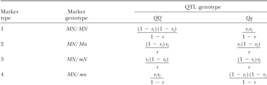
TABLE 1
Conditional probabilities of a putative QTL given flanking marker genotypes for a backcross population
QTL genotype
Marker Marker
type genotype QQ Qq
1 MN/MN (1⫺r1)(1⫺r2)
1⫺r
r1r2
1⫺r
2 MN/Mn (1⫺r1)r2
r
r1(1⫺r2)
r
3 MN/mN r1(1⫺r2)
r
(1⫺r1)r2
r
4 MN/mn r1r2
1⫺r
(1⫺r1)(1⫺r2)
1⫺r
ris the recombination fraction between the two flanking markersMand N. r1(r2) is the recombination
fraction between the putative QTL and the left (right) markerM (N).
and may suffer from the lack of interpretability in terms their differences, a one-QTL model for a backcross
pop-ulation is first used as an example. Their differences
of the genetic model (HaleyandKnott1992;Jansen
1993), it is often claimed that the two approaches pro- under a multiple-QTL model are discussed later. The
one-QTL ML mapping model can be written as vide virtually similar or identical estimates and test
statis-tics in QTL mapping (Haley and Knott 1992; Xu
yi⫽ ⫹axi*⫹εi, i⫽ 1, 2, . . . ,n, (1) 1998a,b). As a consequence, the REG method has been
widely accepted and applied to QTL mapping studies whereyiis the quantitative trait value of individuali,
by many researchers (Haleyet al.1994;Whittakeret is the mean,ais the effect of QTL Q ,x*i, taking a value
al. 1996; Xu 1996, 1998a,b; Goffinet and Mangin 1⁄
2(⫺1⁄2) for homozygoteQQ(heterozygoteQq), denotes
1998;Lebretonet al.1998;DupuisandSiegmund1999; the genotype of Q , andεiis the environmental deviation
RebaiandGoffinet2000). and is assumed to followN(0, 2). Although the
geno-Although REG may approximate ML interval mapping type of Q for an individual is usually unobserved and
well in some cases as shown byHaleyandKnott(1992) could beQQorQq, its distribution can be inferred from
and Xu (1998a,b), their differences in the estimation its flanking marker genotypes. Suppose the flanking
of QTL parameters could be significant for practical markers are M and N. Then, there are four types of
QTL mapping as shown in this article. Unfortunately, marker genotypes, type 1MN/MN, type 2MN/Mn, type
there are few attempts to investigate these differences 3 MN/mN, and type 4 MN/mn, as shown in Table 1.
in the literature.Xu(1995) pointed out that the estima- Given the four marker genotypes, the conditional
prob-tion of residual variance by REG interval mapping is abilities for QTL genotypesQQandQq, denoted bypi1
biased. In this article, the differences between the two andpi2, respectively, at a position between the markers
approaches in the estimation of and testing for QTL can be calculated based on Haldane’s mapping function
parameters due to several factors, such as heritability, (Haldane1919), and they are listed in Table 1.
size of interval, relative QTL position in an interval, the Since the QTL genotypex*i could be homozygote (1⁄
2)
difference between QTL effects, epistasis, and linkage or heterozygote (⫺1⁄
2) for an individual, the likelihood
between QTL, are investigated both analytically and nu- is then a normal mixture with mixing proportions
equiv-merically by simulation. With the understanding of the alent to the conditional probabilities pi1 andpi2. Forn
factors affecting the differences between the two meth- individuals in the sample, the likelihood of the model
ods, a more efficient, precise, and powerful strategy in Equation 1 is
using both methods can be explored in QTL mapping.
The QTL mapping properties under these factors are L(|Y,X)⫽
兿
n
i⫽1
[
兺
2
j⫽1
pijN(ij,2)], (2)
also investigated and discussed.
where denotes parameters (pij, , a, 2), Y and X
denote the trait value and marker genotypes,N(ij,2)
MAXIMUM-LIKELIHOOD INTERVAL MAPPING
denotes the normal density function with meanijand
The differences between the ML and REG interval variance2, and
mappings can be illustrated by investigating the
differ-ences between their estimators of mean, genetic effects,
i1⫽ ⫹
a
are genotypic values ofQQandQq.In estimation, this
z*i ⫽ E(x*i 2|yi,Xi,)⫽
冢
1 2
冣
2
i1⫹
冢
⫺1 2
冣
2
i2 ⫽
1 4 normal mixture model can be treated as an incomplete
data problem (LittleandRubin1987), which regards
are the conditional posterior expectations of x*i and
the QTL genotypexi* as missing data and trait yi and
x*i2 givenyiandXi, respectively. In each iteration, new
markersXias observed data, and the EM algorithm can
estimates of , a, and 2 are obtained in the M-step.
be implemented to maximize the likelihood and obtain
These new estimates are then used to obtain newi1’s
the MLE.
andi2’s for the next iteration. The converged values
Let the probability distribution of missing datax*i as
in the iteration are the MLE. A disadvantage of the EM algorithm was that it did not provide the estimates of
g(x*i )⫽
冦
ppi1 ifx*i ⫽1/2i2 ifx*i ⫽ ⫺1/2. the covariance matrix of the MLE. However, this
disad-vantage can be easily removed by using appropriate The conditional distribution of the observed data,yiand
methods, such as byLouis(1982) andMengandRubin
Xi, given the missing data xi* can be considered as an
(1991), associated with the EM algorithm. The null
hy-independent sample from a population such thatyi|(,
pothesis,H0,a⫽0, for the existence of a QTL is tested
Xi, xi*)ⵑ N( ⫹ axi*, 2), and the EM algorithm can
by a likelihood-ratio test (LRT),⫺2 loge(L0/L1), where
be used to obtain the MLE. At a given position,pij’s can
L0 andL1are the maximum likelihoods under H0 and
be determined. By the definition of the EM algorithm,
no restriction. The larger the LRT statistic at a testing
the iteration of the EM-step for obtaining, a,and2
position, the more likely the existence of a QTL at that proceeds as follows:
position.
E-step:The posterior probabilities of the QTL geno-typesx*i’s of then individuals are updated as
REGRESSION INTERVAL MAPPING
i1 ⫽p(x*i ⫽ 1
2|yi,Xi,)⫽
pi1N(i1,2)
pi1N(i1,2)⫹pi2N(i2,2) HaleyandKnott(1992) commented on ML interval
mapping that the iterative procedure of the EM algo-and
rithm in obtaining the MLE can be complex and compu-tationally slow to converge. Therefore, they developed
i2 ⫽p(x*i ⫽ 1
2|yi,Xi,)⫽
pi2N(i2,2)
pi1N(i1,2)⫹pi2N(i2,2) REG interval mapping to approximate ML interval
map-ping for mapmap-ping QTL. They claimed that the REG
for i ⫽ 1, 2, . . . , n (see Kao and Zeng1997 for the method can ease the computation and produce very
detailed procedure of derivation). Note thati1for indi- similar results as those obtained by the ML method. The
vidual i is a function of pi1, pi2, yi, , a, and 2. It is one-QTL REG interval mapping model for a backcross
important to clarify the relationship between the condi- population can be formulated as
tional probabilitypi1and conditional posterior
probabil-yi⫽ ⫹awi⫹εi, (6)
ityi1of the QTL genotype in the comparison of ML
and REG interval mappings. It is shown later that the
where,a, andεihave the same definitions as the model more similarity betweeni1andpi1for eachi, the better
in Equation 1, and the approximation of REG to ML interval mapping.
Note thatpi1⫽ i1ifpi1⫽1 orpi1⫽0 (i.e., the QTL is
wi⫽E(x*i|Xi)⫽
1 2pi1⫺
1
2pi2⫽ pi1⫺ 1 2 located at the marker) ora ⫽0. Ifpi1 ≈1 orpi2 ≈0 or
a≈0, theni1≈ pi1.
M-step:Find,a, and2to satisfy is the conditional expectation of the QTL genotype
given the flanking marker genotype. By treatingwi as
fixed, the model is a regression model, and this method
⫽1
n
兺
n
i⫽1
(yi⫺w*i a) (3)
is called REG interval mapping in QTL mapping. In estimation, both least-squares and maximum-likelihood
a ⫽
兺
n
i⫽1w*i(yi⫺ )
兺
n i⫽1z*i(4) techniques can be implemented to estimate,a, and
2 in Equation 6. Least-squares estimates (LSE) of
anda are the solutions of
2 ⫽1
n
冤
兺
n
i⫽1
(yi ⫺ )2⫺2(yi⫺ )w*i a⫹ z*ia2
冥
, (5) ⫽1
n
兺
n
i⫽1
(yi⫺wia) (7)
where
a ⫽
兺
n
i⫽1wi(yi⫺ )
兺
n i⫽1zi, (8)
w*i ⫽E(x*i |yi,Xi,)⫽
1 2i1⫺
1
2i2⫽ i1⫺ 1 2
Proportion of variance explained by a QTL: If the
zi ⫽w2i ⫽
冢
pi1⫺1 2
冣
2 ⫽1
4⫺pi1(1⫺pi1). proportion of variance explained by a QTL is small, the
ratio of QTL effectato the environmental deviation
Note that the estimates of the regression model will fail (a/) will be small. Consequently, the densities of
nor-if zi ⫽ 0 (pi1 ⫽ pi2 ⫽ 1|2) for every i. However, this mal mixture components are about the same for
differ-situation will not occur becausepi1⬆pi2for individuals ent genotypes,i.e.,
with type 1 (MN/MN) and type 4 (MN/mn) flanking
N(i1,2)≈N(i2,2)≈N(,2),
marker genotypes in the backcross population. The LSE of2is
andpi1≈i1. The extreme case isa⫽0 (i1⫽ i2⫽ )
andpi1⫽ i1. Therefore, REG mapping can approximate ˆ2⫽ 1
n⫺2
兺
n
i⫽1
[(yi⫺ )2⫺ 2(yi⫺ )wia⫹zia2], (9) ML mapping well when the proportion is low (the QTL
effect a is small). When the proportion is high, QTL
wheren ⫺2 is the degree of freedom for the residual effect a becomes relatively large when compared with
sum of squares. The likelihood of the REG mapping the environmental deviation, and the difference
be-model is a normal density tween the two normal densities can become significant.
As a result, the approximation of REG to ML interval
LREG(|Y,X)⫽
兿
n
i⫽1
N( ⫹awi,2) (10) mapping may not be good for QTL with large effect.
Relative QTL location in an interval:If a QTL is
lo-rather than a normal mixture density. The mixing pro- cated on the boundary of a marker interval,pi1is close
portion ofpij’s in the ML mapping likelihood (Equation to 1 or 0, and the conditional and posterior probabilities
2) is blended intowiof Equation 10. If the maximum- will be similar (pi1≈i1). When the QTL position shifts
likelihood principle is used in estimation, the MLE of from the boundary toward the middle of an interval,pi1
anda for maximizing Equation 10 are the same as and i1 become more dissimilar to each other. If the
Equations 7 and 8. The MLE of2has a divisorninstead
QTL is located in the middle, individuals with type 2
ofn⫺ 2 in Equation 9. or 3 flanking marker genotype havepi1 ⫽ 0.5, and pi1
and i1 will be the most dissimilar. Consequently, the
approximation of REG to ML mapping will be better
DIFFERENCES BETWEEN ML AND
when the QTL is located near the boundary, but it
REG INTERVAL MAPPING
becomes poor as the location moves toward the middle
By comparing the solution sets between ML and REG of an interval.
interval mappings, it can be seen that the two solution Interval size:There are four types of flanking marker
sets have similar expressions, but different contents. In genotypes (Table 1). Types 1 and 4 are
nonrecombi-the REG method, nonrecombi-the conditional expectations of QTL nant, and types 2 and 3 are recombinant. Given a
posi-genotype,wi andzi, are used in estimation. In the ML tion in an interval, the conditional probability pi1 for
method, the conditional posterior expectations of QTL QQ will be closer to 1 or 0, i.e., pi1 can be closer to
genotype,wi* andzi*, play the same role in estimation. i1, for nonrecombinant individuals than recombinant
The conditional expectations consider only the condi- individuals. As there are more nonrecombinant
flank-tional probabilities of QTL genotypespi1’s, and the con- ing genotypes in a narrow interval than in a wider
inter-ditional posterior expectations consider the posterior val, the approximation of REG to ML mapping
conse-probabilitiesi1’s. It can be seen that the posterior prob- quently is better for a QTL located in a narrow interval
abilityi1also utilizes phenotypic information as well as than in a wider interval. Therefore, if QTL are located
marker information. Intuitively, the ML method can in the dense marker region, the differences between
provide better estimates than the REG method because the two methods will be minor.
i1is more informative thanpi1. Analytically, the
differ-ences between ML and REG interval mapping in
estima-MULTIPLE-QTL MODEL
tion will depend on the differences between the two kinds of expectations. The two kinds of expectations
For the one-QTL model, it has been shown that the
are equivalent if and only ifi1⫽pi1andpi1⫽1 (orpi1⫽ approximation of REG to ML interval mapping depends
0) for each i (the QTL is located at a marker). How
on the similarity between the conditional probabilityi1
good the approximation of REG to ML interval mapping
and conditional posterior probabilityi1for eachi.The
is depends on the similarity between pi1’s andi1’s.
In-same argument also applies to the multiple-QTL model. vestigating the factors affecting the similarity between
When multiple, say,mQTL are considered, the multiple
i1andpi1can lead to identifying the differences between interval mapping (MIM;
Kaoet al.1999) model can be
the two methods. These factors include (1) proportion of
written as variance explained by a QTL (size of a QTL), (2) the
relative QTL position within an interval, and (3) the size
yi⫽ ⫹
兺
mj⫽1
ajx*ij ⫹
兺
m
where xij* denotes the genotype of QTL Qj, aj and Ijk plained by QTL, the relative QTL position in an interval, and interval sizes, discussed in the previous section, the
are the main and epistatic effects, ␦jk is an indicator
variable for indicating whether the epistasis between Qj relative sizes of genotypic values of the 2mpossible
geno-types,ij’s, can affect the approximation of REG to ML
and Qkis present or not, and εi is the environmental
deviation. interval mapping in the multiple-QTL model. Ifij’s are
dissimilar to each other (more disperse),ij’s can be
For m QTL, there are 2m possible QTL genotypes;
hence there are 2mcorresponding genotypic values,
ij’s, more dissimilar topij’s, and the differences between the
two methods can become large. The difference between with probabilitiespij’s,j⫽ 1, 2, . . . , 2m. The likelihood
of the multiple-QTL model is then a 2mnormal mixture the sizes of QTL effects and the strength of epistasis
between QTL seems to be an appropriate measure to
L(|Y,X)⫽
兿
n
i⫽1
冤
兺
2mj⫽1
pijN(ij,2)
冥
. (12) quantify the dissimilarity between the 2mgenotypicval-ues. If QTL effects differ from each other significantly or epistasis between QTL is strong,ij’s tend to be dis-It seems that the derivation of the MLE of,a1,a2, . . . ,
similar topij’s. Consequently, the differences between
am,Ijk, and2and their asymptotic variance-covariance
REG and ML interval mapping will be larger if QTL matrix is tedious as the number of QTL considered
effects differ significantly or the interaction between increases in the model. However, this tedious estimation
QTL is strong. problem can be easily solved by the general formulas
If QTL are linked, they are correlated. Their
correla-proposed byKao and Zeng(1997) by expanding the
tion is 1 ⫺ 2r, where r is the recombination fraction
genetic design matrix D and conditional probability
between QTL. As QTL (predictors) in the model are
matrix Q according to the number and positions of
correlated, the effects of collinearity, on modeling such testing QTL. These two matrices play the same role as
as imprecise estimation and losing power in testing for
the matrix of independent variable X in regression.
individual parameters, will occur (Neteret al. 1990).
Given X matrix in multiple regression, the estimates
When detecting closely linked QTL using the multiple-of regression coefficients and the asymptotic
variance-QTL model, the correlations between the conditional covariance matrix can be easily obtained by formulas
expectations of QTL,wij’s, in the REG model tend to
 ⫽(X⬘X)⫺1X⬘YandV⫽(X⬘X)⫺12. Given these two
be higher than those between the conditional posterior
matricesDandQin the multiple-QTL mapping model,
expectations,w*ij’s, in the ML model. As a result, the
the derivation of the MLE and the asymptotic
variance-REG method tends to give estimates with large SD and covariance matrix can be systematically obtained by the
be less powerful in testing for closely linked QTL (to general formulas. Given the testing QTL positions,pij’s
separate closely linked QTL). The closer they are, the can be determined. According to the general formulas,
worse the approximation of the REG to ML method in the E-step, the 2mposterior probabilities of QTL
geno-will be. types fornindividuals,
ij ⫽
pijN(ij,2)
兺
2mj⫽1pijN(ij,2)
; i⫽1, 2, . . . ,n, SIMULATION STUDIES
Simulations were performed to verify the effects of j⫽1, 2, . . . , 2m,
the above factors, such as the proportion of variance
are updated. In the M-step, the solutions of the parame- explained by QTL, interval size, QTL position, the
dif-ter estimation are in the closed form as shown inKao ference between QTL effects, epistasis, and linkage, on
and Zeng (1997). The asymptotic variances of QTL the approximation of REG to ML interval mapping.
positions and effects can also be obtained using the Assume two unlinked epistatic QTL with effects (a1⫽
general formulas. 1,a2 ⫽ 1,I12⫽ 1) that affected a quantitative trait of
The REG interval mapping model for takingmQTL interest in a backcross population (epistasis contributes
into account can be written as 11.11% of the total genetic variation). For simplicity,
10 equally spaced marker intervals were simulated for yi⫽ ⫹
兺
m
j⫽1
ajwij ⫹
兺
m
j⬆k␦jk(Ijkwijwik)⫹ εi. each chromosome. Four proportions of variance
ex-plained by QTL (h2’s), 0.01, 0.1, 0.3, and 0.5, and three
different interval sizes, 10, 20, and 40 cM, are simulated.
In the model,wij is the conditional expectation of Qj
given its flanking markers. The LSE of,a1,a2, . . . ,am, The relative QTL positions are placed in the middle or on the boundary of a marker interval (1, 2, and 4 cM Ijk, and 2 as well as their asymptotic variances can be
obtained using the standard least-squares technique. away from the left marker of the three different spaced
intervals, respectively). When investigating the effect of
Differences due to QTL effects, epistasis, and
link-age:By the same argument, it is required that pij ≈ij epistasis, the main and epistatic QTL effects are further
set at (a1⫽1,a2⫽1,I12⫽2) or (a1⫽1,a2⫽1,I12⫽
for eachiandjfor REG interval mapping to
approxi-mate ML interval mapping well in the multiple-QTL 3), and the QTL are placed in the middle of 40-cM
ex-TABLE 2
Comparison of maximum likelihood and regression interval mapping of simulated data (h2⫽0.5)
Spacing
10 cM 20 cM 40 cM
Mean SD MSE Mean SD MSE Mean SD MSE
⫽0 ML 0.004 0.056 0.003 0.005 0.057 0.003 0.004 0.063 0.004
REG 0.004 0.057 0.003 0.005 0.060 0.004 0.004 0.064 0.004
a1⫽1 ML 1.008 0.117 0.014 1.001 0.121 0.015 0.993 0.142 0.020
REG 1.006 0.121 0.015 1.000 0.125 0.016 0.993 0.156 0.024
a2⫽1 ML 0.996 0.114 0.013 0.997 0.126 0.016 0.998 0.138 0.019
REG 0.997 0.115 0.013 0.997 0.132 0.017 0.998 0.154 0.024
I12⫽1 ML 1.011 0.230 0.053 0.991 0.250 0.063 0.994 0.274 0.075
REG 1.008 0.241 0.058 0.996 0.286 0.082 0.999 0.357 0.127
2⫽0.563 ML 0.551 0.071 0.005 0.549 0.076 0.006 0.552 0.085 0.007
REG 0.614 0.074 0.008 0.670 0.086 0.019 0.782 0.099 0.058
h2⫽0.5 ML 0.511 0.044 0.002 0.510 0.049 0.003 0.509 0.061 0.004
REG 0.452 0.043 0.004 0.399 0.048 0.013 0.302 0.051 0.042
LRT1 ML 80.0 16.1 69.4 15.0 50.9 12.8
REG 75.4 15.5 62.2 14.2 42.1 11.7
LRT2 ML 79.5 14.9 69.2 14.2 51.3 12.6
REG 74.8 14.2 62.0 13.2 42.4 11.3
LRT ML 125.8 16.5 110.5 15.8 82.5 15.1
REG 120.5 16.1 102.4 15.5 72.6 14.4
For each combination of simulated parameters, 500 replicates, each with sample size 200, were analyzed with QTL located in the middle of the marker interval. LRT is the likelihood-ratio test forH0:a1⫽0,a2⫽0,
andI12⫽0. LRT1is the likelihood-ratio test forH0: a1⫽0,I12⫽0, anda2⬆0. LRT2is the likelihood-ratio
test forH0:a2⫽0,I12⫽0, anda1⬆0.h2, the proportion of variance explained by QTL.
quantitative trait variation (the percentages of epistatic of the two methods under various cases. MSE, which is
defined as variance in the total genetic variance are 33.33 and
52.94%, respectively). When investigating the effect of
E(ˆ ⫺ )2⫽ Var(ˆ)⫹[E(ˆ) ⫺ ]2
the difference between QTL effects on the
approxima-tion, five unlinked QTL are placed in the middle of 10- ⫽ Var(ˆ)⫹(Biasˆ)2,
or 40-cM intervals with effects (a1⫽ 1,a2 ⫽1,a3 ⫽ 1,
incorporates two components, one measuring the vari-a4⫽1,a5⫽1), (a1⫽4,a2⫽1,a3⫽1,a4⫽2,a5⫽1),
ability of the estimate (precision), and the other measur-or (a1⫽4,a2⫽1,a3⫽1,a4⫽ ⫺1,a5⫽1), respectively,
ing its bias (accuracy). A good method needs to control and together contribute 50% of the trait variation.
both variance and bias in estimation. When investigating the effect of linkage, two QTL are
As expected, ifh2is low (h2⫽0.01), the two methods
placed in two neighboring 40-cM intervals and are 10,
provide almost identical means and SDs of the estimates 20, 30, or 40 cM apart from each other (5, 10, 15, and
for , a1, a2, I12, 2, and h2, and LRT statistics. These
20 cM from the marker between them). Their effects
results for h2 ⫽ 0.01 correspond with the findings of
are set at (a1⫽ 1,a2 ⫽ ⫺1) without epistasis or (a1 ⫽
Haley and Knott (1992) and Xu (1995, 1998a,b). 1,a2 ⫽ ⫺1,I12⫽ 1) with epistasis, and the heritability
Whenh2becomes higher (h2⬎ 0.1), their differences
is assumed to be 0.1, 0.3, or 0.5 for each case. The
due to the factors of interval size and QTL position sample size is 200, and 500 replicates were simulated
become observable, but minor (the ML method gener-for all cases.
ally has a smaller MSE and larger LRT statistic). To For simplicity of comparison, the QTL positions are
shorten the article, only part of the results are presented, assumed to be known, and the simulation is performed
and the investigation focuses on the factors of linkage, at the positions. When calculating the power of
separat-different QTL sizes, and epistasis under the multiple-ing closely linked QTL, a successful separation requires
QTL model.
the partial LRT statistic for each QTL⬎ 2
1,0.05/10(22,0.05/10
Proportion of variance explained by QTL, interval
for the epistasis case). Means of the estimated parameter
size, and QTL position: The means of the estimated values, their standard deviations (SDs), and mean
main and epistatic effects by the ML and REG methods squared errors (MSEs), as well as the LRT statistics, are
are almost identical and very close to the true values recorded. MSE is used to evaluate the approximation
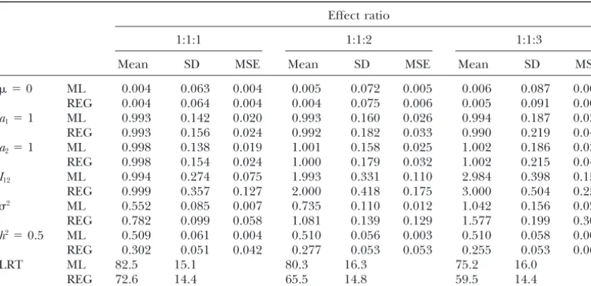
How-TABLE 3
Comparison of maximum likelihood and regression interval mapping of simulated data under different strengths of epistasis
Effect ratio
1:1:1 1:1:2 1:1:3
Mean SD MSE Mean SD MSE Mean SD MSE
⫽0 ML 0.004 0.063 0.004 0.005 0.072 0.005 0.006 0.087 0.008
REG 0.004 0.064 0.004 0.004 0.075 0.006 0.005 0.091 0.008
a1⫽1 ML 0.993 0.142 0.020 0.993 0.160 0.026 0.994 0.187 0.035
REG 0.993 0.156 0.024 0.992 0.182 0.033 0.990 0.219 0.048
a2⫽1 ML 0.998 0.138 0.019 1.001 0.158 0.025 1.002 0.186 0.035
REG 0.998 0.154 0.024 1.000 0.179 0.032 1.002 0.215 0.046
I12 ML 0.994 0.274 0.075 1.993 0.331 0.110 2.984 0.398 0.159
REG 0.999 0.357 0.127 2.000 0.418 0.175 3.000 0.504 0.254
2 ML 0.552 0.085 0.007 0.735 0.110 0.012 1.042 0.156 0.025
REG 0.782 0.099 0.058 1.081 0.139 0.129 1.577 0.199 0.304
h2⫽0.5 ML 0.509 0.061 0.004 0.510 0.056 0.003 0.510 0.058 0.003
REG 0.302 0.051 0.042 0.277 0.053 0.053 0.255 0.053 0.063
LRT ML 82.5 15.1 80.3 16.3 75.2 16.0
REG 72.6 14.4 65.5 14.8 59.5 14.4
For each combination of simulated parameters, 500 replicates, each with sample size 200, were analyzed with QTL located in the middle of a 40-cM marker interval.2⫽0.563 for effect 1:1:1;2⫽0.75 for effect
1:1:2;2⫽1.063 for effect 1:1:3.I
12⫽1, 2, and 3 for the three effect ratios, respectively.h2, the proportion
of variance explained by QTL.
ever, the ML method tends to provide estimates with becomes stronger, the MSEs of the estimates by both
methods become larger, and their differences in MSE smaller SD (MSE) and larger LRT statistics when
com-pared to the REG method. For example, the MSEs of and LRT statistics become larger. For example, the
MSEs of Iˆ12 by the ML method are 0.075, 0.110, and
aˆ1 by the REG method are 0.178, 0.050, and 0.024 for
h2⫽0.1, 0.3, and 0.5, respectively, and the MSEs by the 0.159 for the three ratios, respectively, and they are
0.127, 0.175, and 0.254 by the REG method, respectively. ML method are 0.175, 0.047, and 0.020, respectively
(only the result for h2 ⫽ 0.5 and QTL located in the A similar trend can be observed for other estimates.
The means of LRT statistics for the three ratios are 82.5, middle of the intervals is shown in Table 2). There is a
similar pattern for other estimates. The estimates of2 80.3, and 75.2 for the ML method, respectively, and
they are 72.6, 65.5, and 59.5 for the REG method,
respec-andh2by the REG method are biased, and the estimates
by the ML method are (asymptotically) unbiased. For tively. The bias of the REG method in the estimation of
2andh2also becomes much more serious as interaction
example, thehˆ2by the REG method is 0.072 (SD 0.033),
0.187 (SD 0.047), and 0.302 (SD 0.051) forh2 ⫽ 0.1, between QTL gets stronger. Thehˆ2by the REG method
is 0.302 (SD 0.051), 0.277 (SD 0.053), and 0.255 (SD
0.3, or 0.5, respectively, and thehˆ2by the ML method
is 0.128 (SD 0.055), 0.316 (SD 0.070), and 0.509 (SD 0.053) for the three ratios, respectively (h2⫽0.5). The
ML method, however, can estimateh2and other
parame-0.061), respectively. The bias of the REG method in
estimating 2 and h2 becomes obvious as h2 becomes ters well for all ratios.
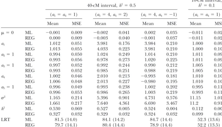
Difference between QTL effects:Table 4 shows the large. Also, the ML method gives larger LRT statistics
than the REG method in all cases. The difference in means, SDs, and MSEs of the estimates as well as the
mean LRT statistics for QTL effects (a1 ⫽ 1, a2 ⫽ 1,
mean LRT statistics between the two methods is
negligi-ble: 0.4 (15.2⫺ 14.8⫽0.4 for 40-cM marker spacing) a3⫽1,a4⫽1,a5⫽1), (a1⫽4,a2⫽1,a3⫽1,a4⫽2,
a5⫽1), and (a1⫽4,a2⫽1,a3⫽ 1,a4⫽ ⫺1,a5⫽1).
forh2⫽0.1 (results not shown), but 9.9 (82.5⫺72.6⫽
9.9 for 40-cM marker spacing) forh2⫽0.5. Therefore, When QTL effects are of the same size, the mean LRT
statistic of the ML method is 1.8 (81.5⫺ 79.7) larger
the difference in the LRT statistic becomes larger ash2
becomes higher. Similar patterns of difference in MSE than that of the REG method. If there are some relatively
large and small QTL, their differences in LRT statistics
and LRT statistics, caused by the change ofh2, can be
observed for other interval sizes and QTL positions. are 3.7 (84.1⫺80.4) and 5.8 (84.7⫺78.9), respectively,
for the other two cases. Also, the estimates by the REG
Epistasis:The means, SDs, and MSEs of the estimates
as well as the mean LRT statistics for effect ratios 1:1:1, method tend to have larger MSEs, and thehˆ2andˆ2by
the REG method are biased. For the case (a1⫽ 1,a2 ⫽
TABLE 4
Comparison of maximum likelihood and regression interval mapping of simulated data under different relative sizes of QTL effects
10-cM interval,
40-cM interval,h2⫽0.5 h2⫽0.1
(a1⫽a4⫽1) (a1⫽4,a4⫽2) (a1⫽4,a4⫽ ⫺1) (a1⫽a4⫽1)
Mean MSE Mean MSE Mean MSE Mean MSE
⫽0 ML ⫺0.001 0.009 ⫺0.002 0.041 0.002 0.035 ⫺0.011 0.022
REG 0.000 0.009 ⫺0.003 0.040 ⫺0.001 0.037 ⫺0.011 0.022
a1 ML 1.012 0.051 3.981 0.176 3.984 0.210 1.000 0.094
REG 1.013 0.055 4.033 0.223 3.981 0.210 1.000 0.100
a2⫽1 ML 0.994 0.050 1.024 0.249 1.014 0.210 1.011 0.094
REG 0.993 0.056 0.978 0.273 1.020 0.225 1.011 0.091
a3⫽1 ML 0.997 0.052 0.992 0.244 0.990 0.212 1.005 0.101
REG 0.993 0.052 0.985 0.251 0.988 0.219 1.005 0.101
a4 ML 1.002 0.046 2.010 0.213 ⫺0.993 0.181 1.010 0.107
REG 1.006 0.048 2.013 0.227 ⫺0.980 0.195 1.010 0.107
a5⫽1 ML 0.996 0.049 0.993 0.238 1.002 0.202 0.995 0.110
REG 0.996 0.053 0.986 0.265 1.003 0.219 0.993 0.111
2 ML 1.165 0.214 5.396 0.901 4.731 0.576 11.15 1.01
REG 1.661 0.217 7.640 4.361 6.690 3.467 11.2 0.919
h2 ML 0.530 0.069 0.527 0.005 0.524 0.004 0.112 0.001
REG 0.327 0.032 0.329 0.032 0.324 0.032 0.099 0.001
LRT ML 81.5 (14.0) 84.1 (14.2) 84.7 (14.4) 52.3 (13.6)
REG 79.7 (14.1) 80.4 (14.4) 78.9 (14.4) 52.2 (13.5)
For each combination of simulated parameters, 500 replicates, each with sample size 200, were analyzed with QTL located in the middle of the marker interval.h2, the proportion of variance explained by QTL.
2⫽1.25 for (a
1⫽1,a2⫽1, a3⫽1,a4⫽1, a5⫽1) andh2⫽0.5.2⫽ 5.75 for (a1⫽4, a2⫽ 1,a3⫽1,
a4⫽2,a5⫽1) andh2⫽0.5.2⫽5.00 for (a1⫽4,a2⫽1,a3⫽1,a4⫽ ⫺1,a5⫽1) andh2⫽0.5.2⫽11.25
for (a1⫽1,a2⫽1,a3⫽1,a4⫽1,a5⫽1) andh2⫽0.1.
1,a3⫽1,a4⫽1,a5⫽1, andh2⫽0.1) and 10-cM intervals, the ML and REG methods are investigated both
analyti-cally and numerianalyti-cally. It is found that the REG method the difference in mean LRT statistic between the two
methods is at a very micro level (52.3⫺52.2⫽0.08). tends to give estimates with larger MSE and smaller LRT
statistics in testing parameters, and it is less powerful in
Linkage:The powers of separating 10-, 20-, 30-, and
40-cM-apart QTL are 97.2, 99.0, 99.6, and 99.8% for the QTL detection when compared with the ML method.
Also, the REG method is biased in estimating the resid-ML method, respectively, and are 22.0, 60.0, 91.6, and
98.4% for the REG method, respectively (Table 5 and ual variance and the proportion of total variance
ex-plained by QTL. Therefore, ML interval mapping is Figure 1). Also, the difference in MSE between the two
methods becomes larger as QTL get closer. The MSE more accurate, precise, and powerful than REG interval
ratios ofaˆ1for the two methods are 4.52 (0.226/0.050), mapping in QTL mapping. The differences in power,
8.67 (0.091/0.011), 4.00 (0.056/0.014), and 2.57 (0.036/ MSE, and LRT statistics between the two methods
de-0.011), respectively (Figure 1c). The estimatedh2by the pend on factors such as size of QTL effect, interval size,
REG method is seriously biased. The means ofhˆ2by the relative QTL position in an interval, difference between
REG method are 0.037, 0.070, 0.112, and 0.162 for QTL effects, epistasis, and linkage between QTL, as
10-, 20-, 30-, and 40-cM-apart QTL, respectively (h2 ⫽ shown in the article. Their differences in general may
0.5). The ML method, however, can estimate h2 well be minor, but can be significant in certain situations.
(see also Figure 1c). Ifh2 ⫽0.3 or 0.1, the power, the
The differences become larger as the proportion
ex-MSE ratio ofaˆ1, andhˆ2for the two methods are shown plained by QTL becomes higher, marker interval becomes
in Figure 1, a–c. If the linked QTL show epistasis, the wider, QTL position moves from boundary to middle
advantage gained by the ML method becomes even of an interval, the difference of QTL effects is larger,
more significant (Figure 1d). epistasis becomes stronger, and the QTL positions are
closer. Especially, the REG method may have a serious problem in detecting closely linked QTL when
com-CONCLUSION AND DISCUSSION
pared with the ML method. As shown in Table 5 and Figure 1, the difference in detecting closely linked In this article, the differences in QTL parameter
TABLE 5
Comparison of maximum likelihood and regression interval mapping of simulated data under different strengths of linkage
Distance between QTL
10 cM 20 cM 30 cM 40 cM
Mean MSE Mean MSE Mean MSE Mean MSE
⫽0 ML 0.001 0.001 0.000 0.001 0.000 0.002 0.000 0.002
REG 0.000 0.008 ⫺0.001 0.002 0.001 0.002 0.001 0.002
a1⫽1 ML 0.974 0.050 1.002 0.011 0.994 0.014 0.996 0.011
REG 1.002 0.226 1.005 0.091 1.005 0.056 0.999 0.036
a2⫽ ⫺1 ML ⫺0.972 0.051 ⫺1.002 0.011 ⫺0.994 0.013 ⫺0.995 0.014
REG ⫺1.002 0.228 ⫺1.005 0.090 ⫺1.005 0.057 ⫺0.998 0.036
h2⫽0.5 ML 0.496 0.007 0.508 0.005 0.507 0.006 0.510 0.006
REG 0.037 0.217 0.070 0.186 0.112 0.152 0.162 0.116
LRT ML 42.0 (16.1) 32.7 (11.0) 36.6 (11.0) 46.0 (12.4)
REG 6.7 (5.1) 13.5 (7.1) 21.6 (9.0) 30.6 (10.5)
LRT1 ML 40.9 (16.1) 31.2 (10.8) 33.7 (10.6) 39.9 (11.4)
REG 7.7 (5.4) 14.7 (7.2) 24.0 (9.3) 35.6 (11.4)
LRT2 ML 40.9 (16.1) 31.3 (11.0) 33.8 (10.9) 40.0 (11.7)
REG 6.7 (5.1) 13.4 (6.9) 21.5 (9.0) 30.5 (10.5)
Power (%) ML 97.2 99.0 99.6 99.8
REG 22.0 60.0 91.6 98.4
For each combination of simulated parameters, 500 replicates, each with sample size 200, were analyzed with two QTL contributing 50% of the total genetic variance and located in the middle of the marker interval. LRT is the likelihood ratio test forH0:a1⫽0 anda2⫽0. LRT1is the likelihood ratio test forH0:a1⫽0 and
a2⬆0. LRT2is the likelihood ratio test forH0:a2⫽0 anda1⬆0. Power, percentage of replicates with LRT1
⬎7.88 and LRT2⬎7.88. Numbers in parentheses denote standard deviation.h2, the proportion of variance
explained by QTL.
significant (power 0.22 vs. 0.97 for 10-cM-apart QTL tors as shown in this article. Using the multiple-QTL
model of the ML approach, it has been found that
and h2 ⫽ 0.5; power 0.60 vs. 0.99 for 20-cM-apart
QTL andh2⫽0.5; power 0.09vs.0.54 for 10-cM-apart quantitative traits with a somewhat medium to high
heri-tability might be affected by several linked and unlinked
QTL and h2 ⫽ 0.3; power 0.34 vs. 0.61 for
20-cM-apart QTL andh2⫽0.3). In addition, the REG method is QTL, having different sizes, directions, and interaction
of effects (Kao et al. 1999;Weber et al. 1999;Zenget
seriously biased in estimating the proportion of variance
explained by QTL (Figure 1b), and it gives the estimates al.2000). Also, the linkage map may have wide marker
intervals (Grattapaglia et al. 1996;Satagopanet al.
of the effects with much larger MSEs (Figure 1c). The
problem of the REG method in detecting closely linked 1996; Li et al.1997; Kao et al.1999). As a result, the
REG method can be significantly different from the QTL becomes worse if epistasis is present (Figure 1d).
It was often pointed out that there is no significant ML method and thus be problematic in practical QTL
mapping. difference in the estimation of QTL parameter and
sta-tistical power of QTL detection between the REG and The cost in computation per iteration in the EM
algo-rithm is generally not very expensive (McLachlanand
ML methods with the exception that the estimate of
residual variance by the REG method is biased (Haley Krishnan 1997). If the model is extended to fit five
QTL, the ML method needsⵑ18 iterations to converge
and Knott 1992; Xu 1995, 1998a,b). These findings
were mostly done by simulation and concentrated on and is⬍10 times slower than the REG method for the
40-cM interval case (the REG method takesⵑ65 sec and
the comparison of mean estimate (accuracy) of QTL
effect for low heritability (h2⫽0, 0.008, 0.03, and 0.111 the ML method takesⵑ608 sec to finish the
computa-tion of 500 replicates). Therefore, the ML method inHaleyand Knott1992) and a QTL positioned in
a narrow interval (interval size 10 cM inXu 1998a,b) should not be regarded as formidably expensive in
com-putation as the computer technology is advancing.Xu
for a one-QTL model. Therefore, their differences due
to factors such as different QTL sizes, epistasis, and (1998a,b) proposed the iteratively reweighted
least-squares (IRWLS) method to correct the bias of the REG linkage between QTL had not been identified and
needed to be checked using the multiple-QTL model. method in estimating residual variance. The estimates
by both REG and IRWLS methods tend to have larger When multiple QTL are considered simultaneously in
the model, the differences in power and estimation be- SD than those by the ML method (Tables 1–4 in Xu
1998a; Table 7 in Xu 1998b). As the MLEs have the
fac-Figure1.—The power, estimate of proportion of variance ex-plained by QTL (h2), and MSE of
effect estimate by the ML and REG methods in the analysis of two linked QTL without (a1⫽1,a2⫽
⫺1) and with (a1⫽ 1, a2 ⫽ ⫺1,
I12⫽1) epistasis under different
genetic distances and proportions of variance explained by QTL (h2).
(a) Power of separating two linked QTL with no epistasis. The solid lines from bottom to top denote the power by the ML method for h2⫽0.1, 0.3, and 0.5, respectively.
The dotted lines from bottom to top denote the power by the REG method forh2⫽0.1, 0.3, and 0.5,
respectively. (b) Estimate of h2.
The solid lines from bottom to top denote the estimate of h2by the
ML method forh2⫽0.1, 0.3, and
0.5, respectively. The dotted lines from bottom to top denote the es-timate of h2by the REG method
forh2⫽0.1, 0.3, and 0.5,
respec-tively. (c) Ratio of MSE. The solid, dotted, and dashed lines from bot-tom to top denote the MSE ratio ofaˆ1by the REG method and ML
method for h2⫽0.1, 0.3, and 0.5,
respectively. (d) Power of separat-ing two linked QTL with epistasis. The solid lines from bottom to top denote the power by the ML method forh2⫽0.1, 0.3, and 0.5,
respectively. The dotted lines from bottom to top denote the power by the REG method forh2⫽
0.1, 0.3, and 0.5, respectively.
property of asymptotical efficiency, it should not be residual error does not follow normal distribution, the
mixture model in Equation 2 should take its specific surprising that the ML method has the ability to provide
the smallest SD among estimates (CasellaandBerger form into account to model the relation between the
quantitative trait and QTL in estimation. In practice, 1990). Therefore, ML interval mapping is not only a
more powerful but also a more precise method in QTL although most of the residual errors are normally
dis-tributed and the use of the normal mixture model mapping.
The distributions of most quantitative traits approxi- should be safe in most situations, it is important to
examine the pattern of residuals, which is a requisite mate more or less close to normal or can be scaled to
normal through simple transformation (Falconerand procedure in model selection, to ensure that the final
QTL mapping model is appropriate.
Mackay 1996). Therefore, when mapping QTL, the
likelihood is generally modeled as a normal mixture The QTL mapping result will be used as a base for
follow-up operations, such as marker-assisted selection (Equation 2). When applying the EM algorithm to the
estimation of a normal mixture model, the estimating or gene transfer, on QTL for trait improvement. To
ensure the validity of trait improvement, the quality of Equations 3, 4, and 5 depend on the conditional
poste-rior probabilities of QTL genotypesij’s, which take the QTL mapping should be more important than the ease
of computation. Researchers using the REG method for distribution of the residual error into account using
normal density. The estimation of the REG method mapping QTL need to be concerned with the factors
affecting its approximation to the ML method in
prac-depends on the conditional probabilities pij’s, which
ignore the distribution of residual error, and the IRWLS tice. For example, if there are wide marker intervals
along the genome (known data structure), or the QTL method takes only the second moment of residual error
into account whatever the underlying residual error dis- effects are not sure to be equally small, or the QTL are
linked with epistasis (unknown QTL parameters), the tribution is. This is also the reason why the ML method
Jansen, R. C.,1993 Interval mapping of multiple quantitative trait
the ML method. Then, after the analysis of the REG
loci. Genetics135:205–211.
method, there is a need to further use the ML method Jiang, C.,andZ.-B. Zeng,1997 Multiple trait analysis of genetic
mapping for quantitative trait loci. Genetics140:1111–1127.
to finalize the QTL mapping result. As far as
computa-Kao, C.-H.,andZ.-B. Zeng,1997 General formulas for obtaining the
tion is concerned, it is suggested that researchers may MLE and the asymptotic variance-covariance matrix in mapping
use the REG method as an initial procedure to obtain quantitative trait loci when using the EM algorithm. Biometrics
53:359–371.
preliminary results and further use the ML method as
Kao, C.-H., Z.-B. ZengandR. D. Teasdale,1999 Multiple interval
a final procedure to obtain the conclusive results of mapping for quantitative trait loci. Genetics152:1203–1216.
QTL mapping. Lander, E. S.,andD. Botstein,1989 Mapping Mendelian factors
underlying quantitative traits using RFLP linkage maps. Genetics This study was supported by grants NCS89-2313-B-001-006 from the 121:185–199.
National Science Council, Taiwan, Republic of China. Lebreton, C. M., P. M. Visscher, C. S. Haley, A. Semikhodskiiand
S. A. Quarrie, 1998 A nonparametric bootstrap method for testing close linkagevs.pleiotropy of coincident quantitative trait loci. Genetics150:931–943.
Li, Z., S. R. M. Pinson, W. D. Park, A. H. PatersonandJ. W. Stansel,
LITERATURE CITED 1997 Epistasis for three grain yield components in rice (Oryza sativa L.). Genetics145:453–465.
Carbonell, E. A., T. M. Gerig, E. BalansardandM. J. Asins,1992
Little, R. J. A.,andD. B. Rubin,1987 Statistical Analysis With Missing Interval mapping in the analysis of nonadditive quantitative trait
Data.John Wiley, New York. loci. Biometrics48:305–315.
Louis, T. A.,1982 Finding the observed information matrix when
Casella, G.,andR. Berger, 1990 Statistical Inference. Wadsworth,
using the EM algorithm. J. R. Stat. Soc. Ser. B44:226–233. Belmont, CA.
Martinez, O.,andR. N. Curnow, 1992 Estimating the locations
Dempster, A. P., N. M. LairdandD. B. Rubin,1977 Maximum
and the sizes of the effects of quantitative trait loci using flanking likelihood from incomplete data via the EM algorithm. J. R. Stat.
markers. Theor. Appl. Genet.85:480–488.
Soc.39:1–38. McLachlan, G. F.,andT. Krishnan,1997 The EM Algorithm and
Doerge, R. W.,andG. A. Churchill,1996 Permutation test for Extensions.John Wiley, New York.
multiple loci affecting a quantitative character. Genetics 142: Meng, X.-L.,andB. Rubin,1991 Using EM to obtain asymptotic
284–294. variance-covariance matrix: the SEM algorithm. J. Am. Stat. Assoc.
Dupuis, J.,andD. Siegmund,1999 Statistical methods for mapping 86:899–909.
quantitative trait loci from a dense set of markers. Genetics151: Neter, J., W. WassermanandM. H. Kutner,1990 Applied Linear
373–386. Statistical Model.Richard D. Irwin, Tokyo.
Falconer, D. S.,andT. F. C. Mackay,1996 Introduction to Quantita- Rebai, A.,andB. Goffinet,2000 More about quantitative trait locus tive Genetics.Longman Group, London. mapping with diallel designs. Genet. Res.75:243–247.
Goffinet, B.,andB. Mangin,1998 Comparing methods to detect Satagopan, J. M., B. S. Yandell, M. A. NewtonandT. C. Osborn,
more than one QTL on a chromosome. Theor. Appl. Genet.96: 1996 A Bayesian approach to detect quantitative trait loci using
628–633. Markov chain Monte Carlo. Genetics144:805–816.
Grattapaglia, D., F. L. G. Bertolucci, R. PenchelandR. R. Seder- Sillanpaa, M. J.,andE. Arjas,1999 Bayesian mapping of multiple
off,1996 Genetic mapping of quantitative trait loci controlling quantitative trait loci from incomplete outbred offspring data. Genetics151:1605–1619.
growth and wood quality traits inEucalyptus grandisusing a
mater-Song, J. Z., M. SollerandA. Genizi,1999 The full-sib intercross nal half-sib family and RAPD markers. Genetics144:1205–1214.
line (FSIL): a QTL mapping design for outcross species. Genet.
Hackett, C. A.,andJ. I. Weller,1995 Genetic mapping of
quantita-Res.77:61–73. tive trait loci for traits with ordinal distributions. Biometrics51:
Weber, K., R. Eisman, L. Morey, A. Patty, J. Sparkset al., 1999 1252–1263.
An analysis of polygenes affecting wing shape on Chromosome
Haldane, J. B. S.,1919 The combination of linkage values and the
3 in Drosophila melanogaster. Genetics153:773–786. calculation of distances between the loci of linked factors. J.
Whittaker, J. C., R. ThompsonandP. M. Visscher,1996 On the Genet.8:299–309.
mapping of QTL by regression of phenotype on marker type.
Haley, C. S.,andS. A. Knott,1992 A simple regression method
Heredity77:23–32. for mapping quantitative trait loci in line crosses using flanking
Xu, S.,1995 A comment on the simple regression method for inter-markers. Heredity69:315–324.
val mapping. Genetics141:1657–1659.
Haley, C. S., S. A. KnottandJ.-M. Elsen,1994 Mapping
quantita-Xu, S.,1996 Mapping quantitative trait loci using four-way crosses. tive trait loci in crosses between outbred lines using least squares.
Genet. Res.68:175–181. Genetics136:1195–1207.
Xu, S.,1998a Further investigation on the regression method of
Henshall, J. M.,andM. E. Goddard,1999 Multiple-trait mapping
mapping quantitative trait loci. Heredity80:364–373.
of quantitative trait loci after selective genotyping using logistic Xu, S.,1998b Iteratively reweighted least squares mapping for quan-regression. Genetics151:885–894. titative trait loci. Behav. Genet.28:341–355.
Hoeschele, I.,andP. VanRaden,1993a Bayesian analysis of linkage Zeng, Z.-B.,1994 Precision mapping of quantitative trait loci. Genet-between genetic markers and quantitative trait loci. I. Prior knowl- ics136:1457–1468.
edge. Theor. Appl. Genet.85:953–960. Zeng, Z.-B., J. Liu, L. F. Stam, C.-H. Kao, J. M. Merceret al., 2000
Hoeschele, I.,andP. VanRaden,1993b Bayesian analysis of linkage Genetic architecture of a morphological shape difference be-between genetic markers and quantitative trait loci. II. Combining tween two Drosophila species. Genetics154:299–310.
prior knowledge with experimental evidence. Theor. Appl.